

Planning Strategies for Distributed PV-Storage Using a Distribution Network Based on Load Time Sequence Characteristics Partitioning
Abstract
:1. Introduction
2. Partitioning Method and Formulations
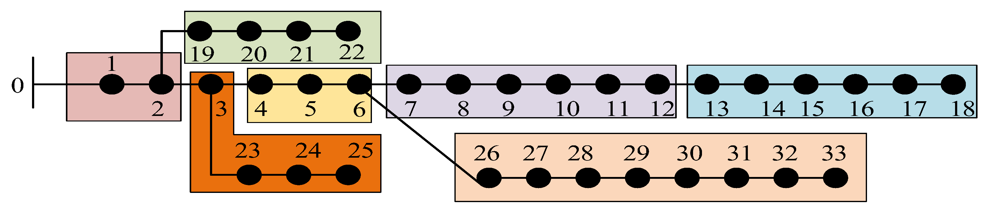
2.1. Partition of Active Distribution Network
Sensitivity of Active and Reactive Power for Conventional Voltages
2.2. Active and Reactive Sensitivity of Sequential Voltage
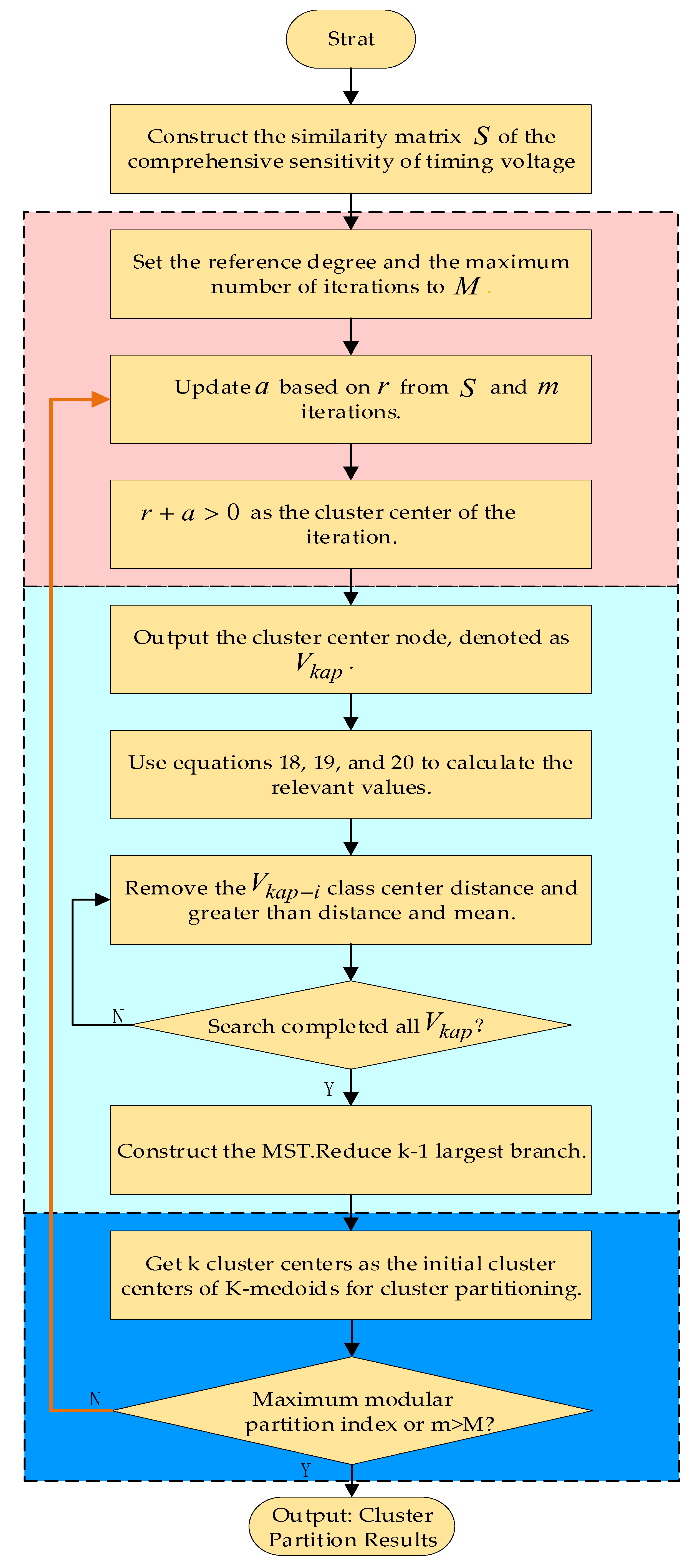
2.3. Distribution Network Partition of the AP-TD-K-Medoids Algorithm
2.4. Evaluation Index of Partition Modularity
3. Planning Method and Modelling
3.1. Upper-Level Planning Model
3.1.1. Objective Function
- Annual cost of investment constructionwhere is the number of partitions. is the discount rate, which is 0.06, is the planning period, 20 years for DPG and 10 years for ESS, , , and are the per-unit capacity of DPG, investment construction cost of ESS, and the unit power investment cost of ESS, respectively, and , , and are the rated capacity of DPG, the rated capacity, and the power of the ESS in the intrapartition , respectively.
- Annual cost of operation maintenancewhere is the power generation of partition at time of DG, and are the charging and discharging power of ESS of partition at time , and , , and are DPG, ESS unit maintenance cost, and DPG curtailment cost, respectively.
- Annual power purchasing costwhere is the number of link branches in the main network and is the power connected to branch through the main network at time .
- Annual government subsidywhere is the government subsidy fee for DPG unit power generation, and is DG power generation efficiency.
3.1.2. Constraints
- DPG capacity and power output constraints of partitionwhere is the number of partitions, is the number of nodes in partition , is the installed capacity of DPG in partition , is the maximum capacity of the DPG installed on node in partition , and is the active power of DPG in partition at time .
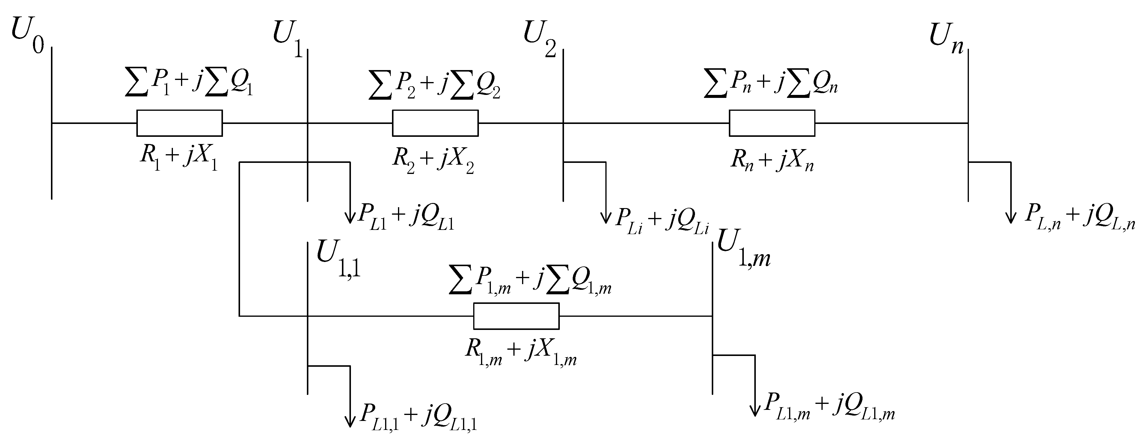
- Power balancewhere is the number of link branches in the main network, is the number of distribution network branches, is the load active power of the node the partition at time , and is the network loss of branch transmitted from the lower level to the upper level at time .
- Constraints on the reverse transmission power of the main network link branchwhere is the maximum reverse transmission power that is allowed by the main network link branch to pass.
- Interpartition interaction branch powerwhere is the number of interpartition interaction branches, and is the maximum power allowed by interpartition interaction branch .
- Power constraints of ESSwhere is the maximum output power of ESS in partition .
- Charge and discharge efficiency constraintswhere is discharge efficiency, and is charging efficiency.
- State-of-Charge (SOC) constraint of the ESSwhere is the state of charge in partition at time , and are the upper and lower limits of the state of charge, and is the initial state of charge.
3.2. Lower-Level Planning Model
3.2.1. Objective Function
3.2.2. Constraints
- 1.
- Power flow constraints
- 2.
- DPG installation capacity constraints of each node of the intrapartition
- 3.
- DPG node installation capacity constraints
- 4.
- Voltage constraints in the partition
- 5.
- Line transmission power constraints of the intrapartition
3.3. Planning and Operation Evaluation Indicators
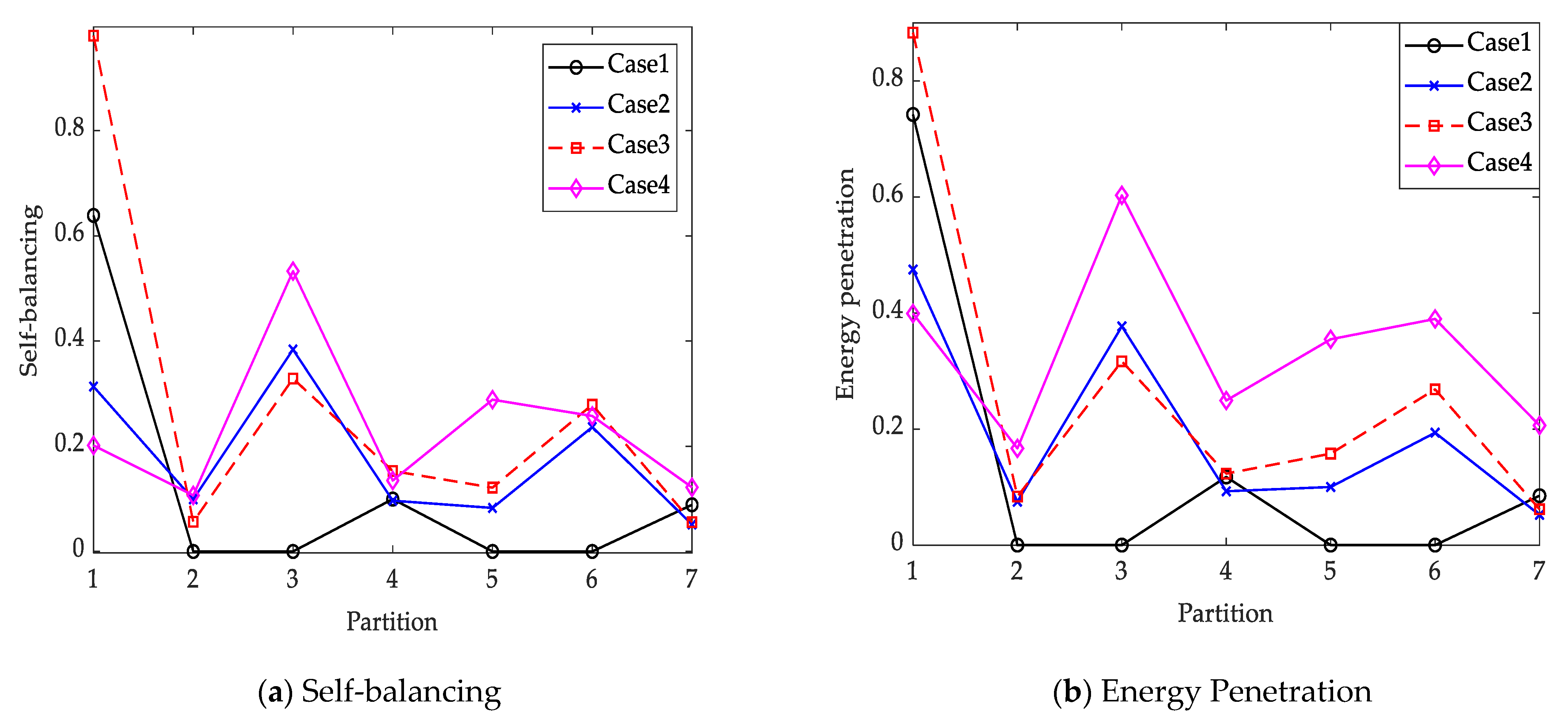
3.3.1. Self-Balancing Degree
3.3.2. Energy Penetration
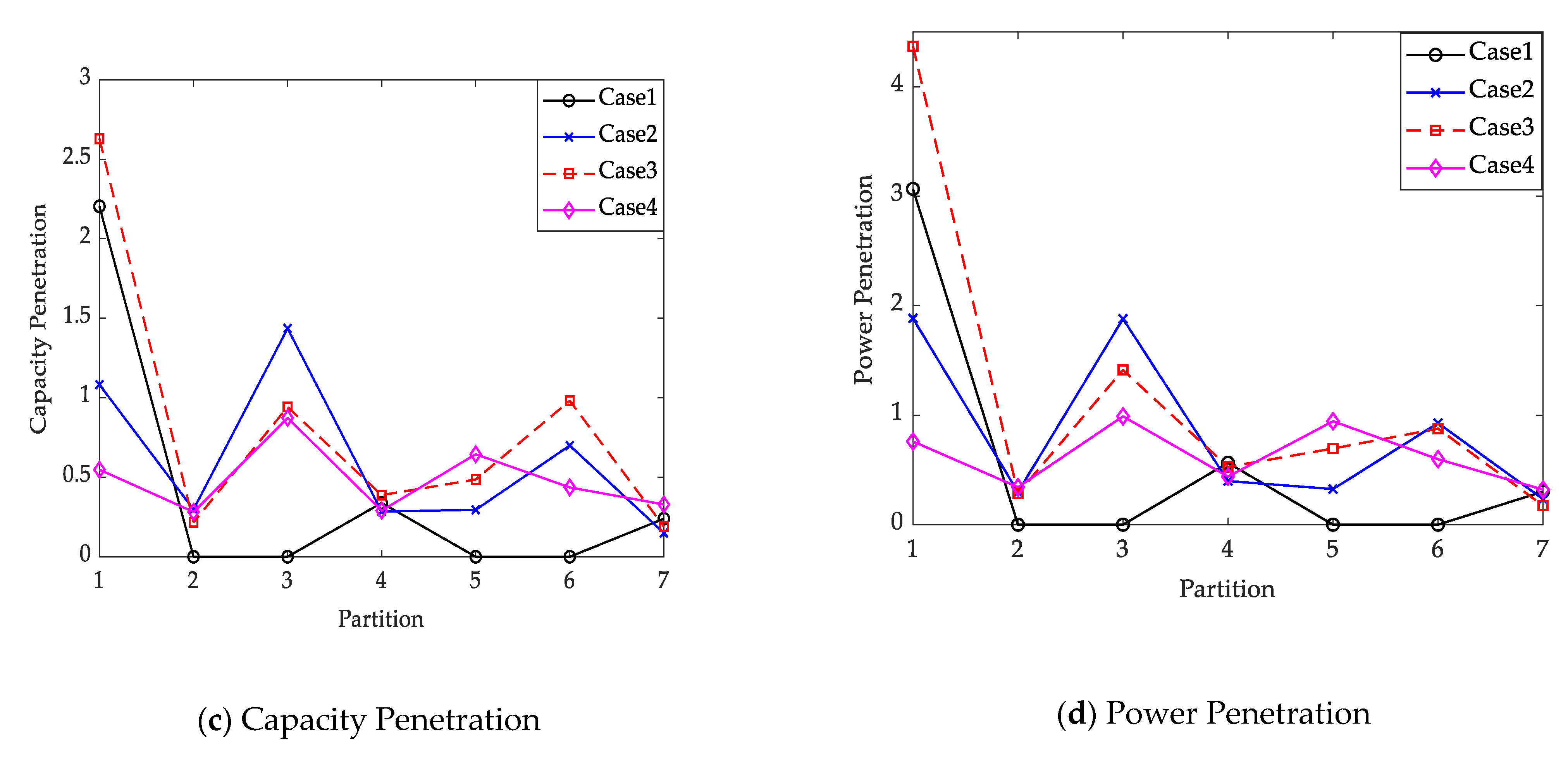
3.3.3. Capacity Penetration
3.3.4. Power Penetration
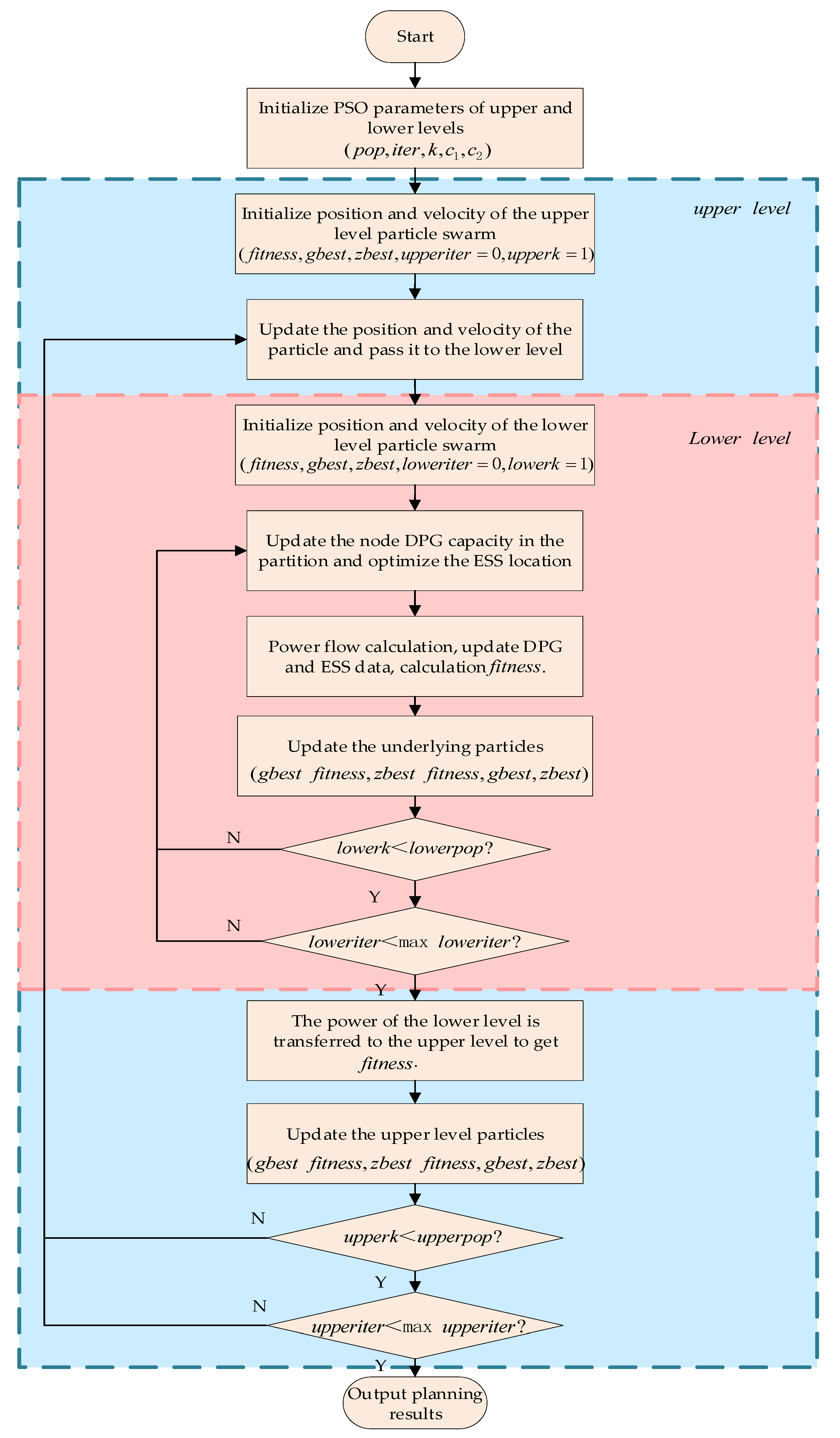
3.4. Bilevel Model Solution Method
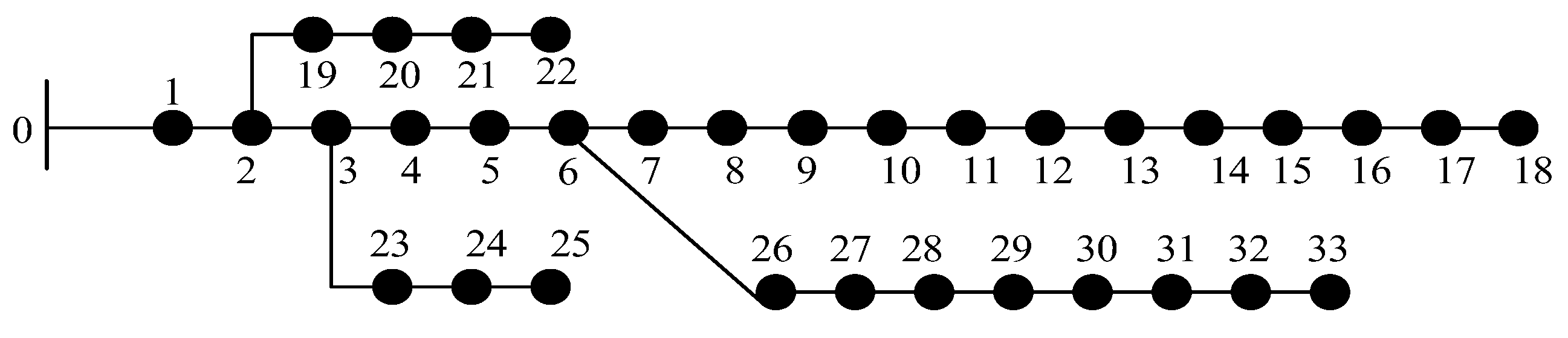
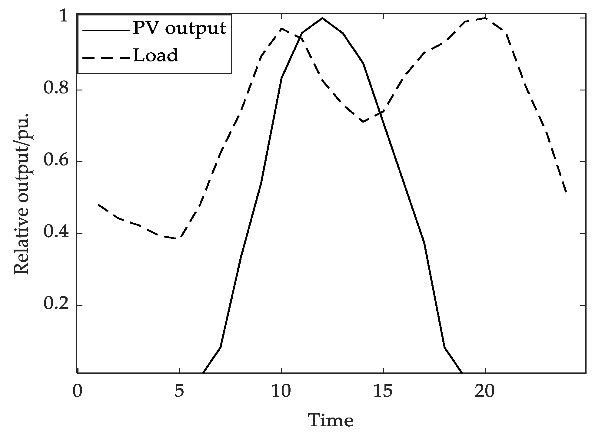
4. Case Study
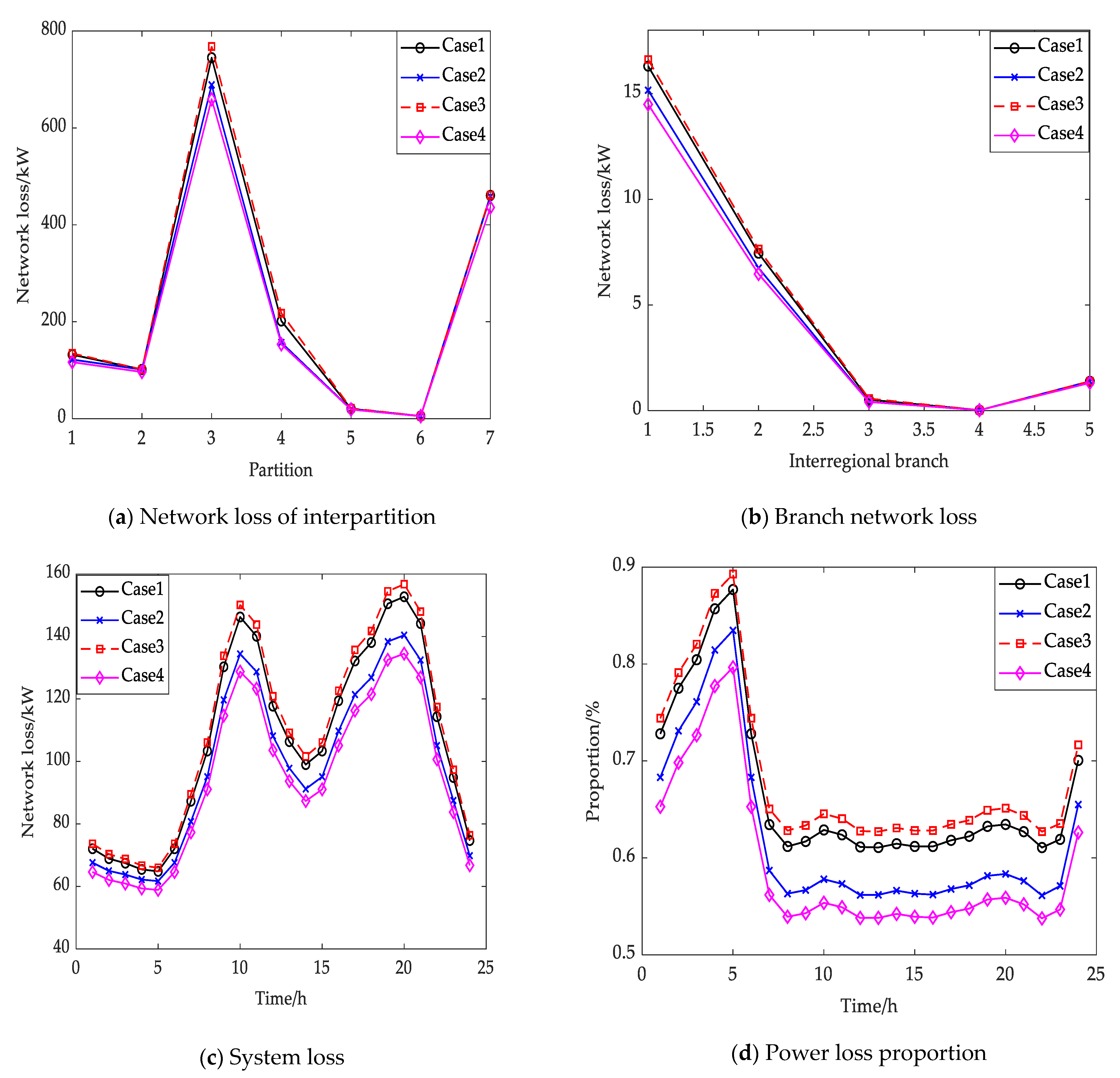
5. Results and Discussion
5.1. DPG and ESS Siting and Sizing Selection Cases
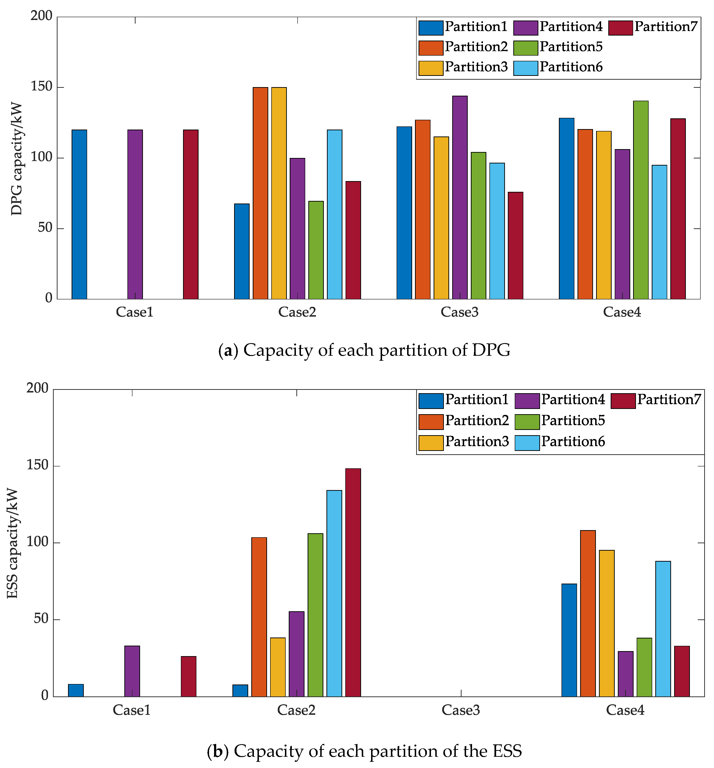
5.2. Upper-Level Planning Results
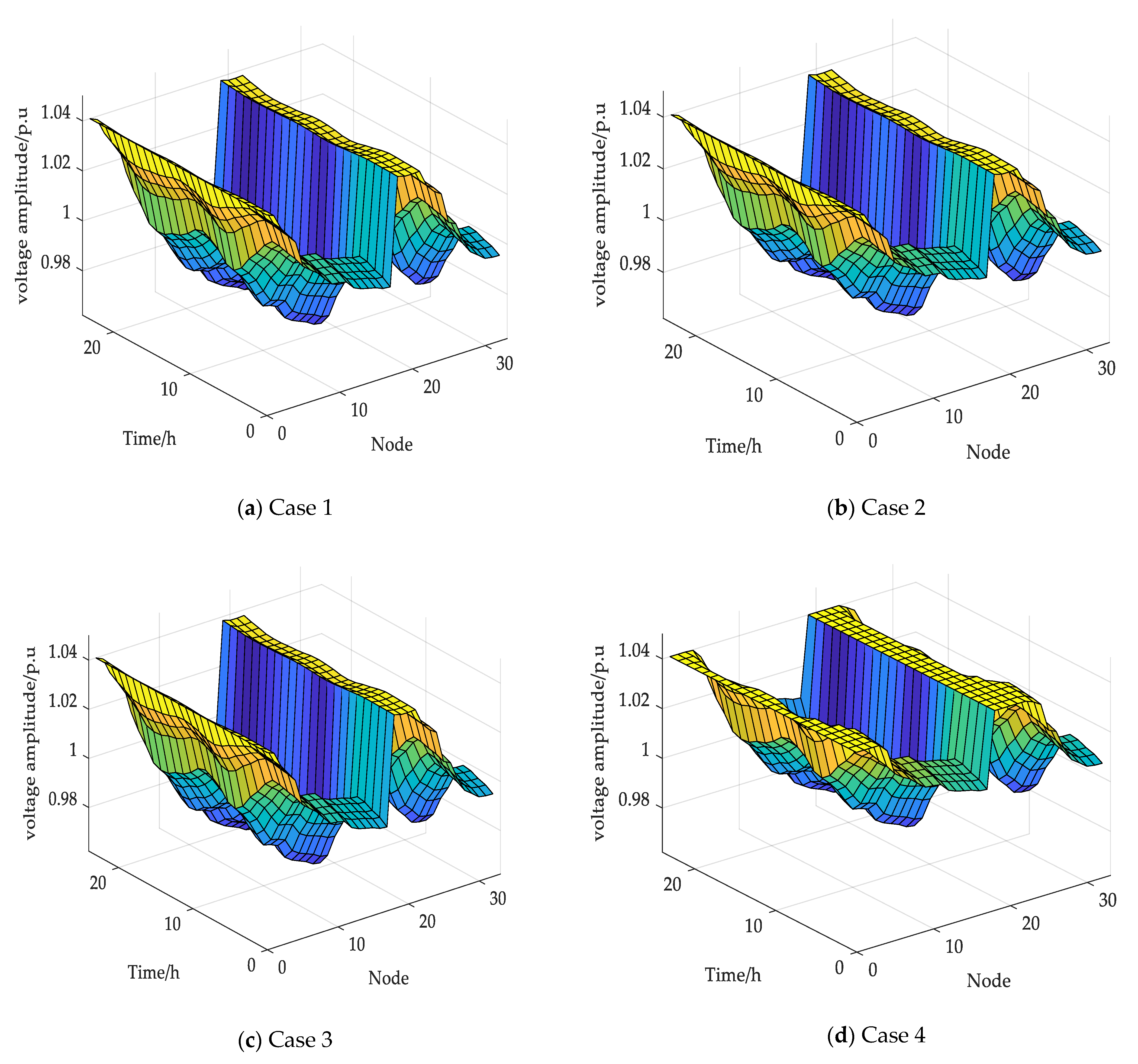
5.3. Lower-Level Planning Results
5.4. Evaluation Indicators for Planning and Operation
6. Conclusions
Author Contributions
Funding
Institutional Review Board Statement
Informed Consent Statement
Data Availability Statement
Conflicts of Interest
References
- Lema, M.; Pavon, W.; Ortiz, L.; Asiedu-Asante, A.B.; Simani, S. Controller Coordination Strategy for DC Microgrid Using Distributed Predictive Control Improving Voltage Stability. Energies 2022, 15, 5442. [Google Scholar] [CrossRef]
- Zhou, J.; Li, Y.; Tian, J.; Ma, Z. The Spatial Effect and Threshold Characteristics of Green Technological Innovation on the Environmental Pollution of Thermal Power, etc., Air Pollution-Intensive Industrial Agglomeration in China. Processes 2022, 11, 43. [Google Scholar] [CrossRef]
- Mufutau Opeyemi, B. Path to sustainable energy consumption: The possibility of substituting renewable energy for non-renewable energy. Energy 2021, 228, 120519–120526. [Google Scholar] [CrossRef]
- Bhukya, L.; Nandiraju, S. A novel photovoltaic maximum power point tracking technique based on grasshopper optimized fuzzy logic approach. Int. J. Hydrog. Energy 2020, 45, 9416–9427. [Google Scholar] [CrossRef]
- Liu, H.; Zhang, J.; Wang, J. Special Issue on “Modeling, Analysis and Control Processes of New Energy Power Systems”. Processes 2023, 11, 235. [Google Scholar] [CrossRef]
- Gitelman, L.; Kozhevnikov, M. Energy Transition Manifesto: A Contribution towards the Discourse on the Specifics Amid Energy Crisis. Energies 2022, 15, 9199. [Google Scholar] [CrossRef]
- Pavon, W.; Inga, E.; Simani, S.; Nonato, M. A Review on Optimal Control for the Smart Grid Electrical Substation Enhancing Transition Stability. Energies 2021, 14, 8451. [Google Scholar] [CrossRef]
- Gao, Y.; Xue, F.; Yang, W.; Yang, Q.; Sun, Y.; Sun, Y.; Liang, H.; Li, P. Optimal operation modes of photovoltaic-battery energy storage system based power plants considering typical scenarios. Prot. Control Mod. Power Syst. 2017, 2, 36. [Google Scholar] [CrossRef]
- Denholm, P.; Arent, D.J.; Baldwin, S.F.; Bilello, D.E.; Brinkman, G.L.; Cochran, J.M.; Cole, W.J.; Frew, B.; Gevorgian, V.; Heeter, J.; et al. The challenges of achieving a 100% renewable electricity system in the United States. Joule 2021, 5, 1331–1352. [Google Scholar] [CrossRef]
- Zhang, S.; Cheng, H.; Li, K.; Bazargan, M.; Yao, L. Optimal siting and sizing of intermittent distributed generators in distribution system. IEEJ Trans. Electr. Electron. Eng. 2015, 10, 628–635. [Google Scholar] [CrossRef]
- Giannitrapani, A.; Paoletti, S.; Vicino, A.; Zarrilli, D. Optimal Allocation of Energy Storage Systems for Voltage Control in LV Distribution Networks. IEEE Trans. Smart Grid 2017, 8, 2859–2870. [Google Scholar] [CrossRef]
- Balu, K.; Mukherjee, V. Optimal siting and sizing of distributed generation in radial distribution system using a novel student psychology-based optimization algorithm. Neural Comput. Appl. 2021, 33, 15639–15667. [Google Scholar] [CrossRef]
- Gao, Y.; Hu, X.; Yang, W.; Liang, H.; Li, P. Multi-Objective Bilevel Coordinated Planning of Distributed Generation and Distribution Network Frame Based on Multiscenario Technique Considering Timing Characteristics. IEEE Trans. Sustain. Energy 2017, 8, 1415–1429. [Google Scholar] [CrossRef]
- Xiao, J.; Zhang, Z.; Bai, L.; Liang, H. Determination of the optimal installation site and capacity of battery energy storage system in distribution network integrated with distributed generation. IET Gener. Transm. Distrib. 2016, 10, 601–607. [Google Scholar] [CrossRef]
- Shaker, H.; Zareipour, H.; Wood, D. Impacts of large-scale wind and solar power integration on California׳s net electrical load. Renew. Sustain. Energy Rev. 2016, 58, 761–774. [Google Scholar] [CrossRef]
- Shaner, M.R.; Davis, S.J.; Lewis, N.S.; Caldeira, K. Geophysical constraints on the reliability of solar and wind power in the United States. Energy Environ. Sci. 2018, 11, 914–925. [Google Scholar] [CrossRef]
- Payne, J.; Gu, F.; Razeghi, G.; Brouwer, J.; Samuelsen, S. Dynamics of high penetration photovoltaic systems in distribution circuits with legacy voltage regulation devices. Int. J. Electr. Power Energy Syst. 2021, 124, 106388–106400. [Google Scholar] [CrossRef]
- Zhao, B.; Xu, Z.; Xu, C.; Wang, C.; Lin, F. Network Partition-Based Zonal Voltage Control for Distribution Networks with Distributed PV Systems. IEEE Trans. Smart Grid 2018, 9, 4087–4098. [Google Scholar] [CrossRef]
- Kwag, K.; Shin, H.; Oh, H.; Yun, S.; Kim, T.H.; Hwang, P.-I.; Kim, W. Bilevel programming approach for the quantitative analysis of renewable portfolio standards considering the electricity market. Energy 2023, 263, 126013–126025. [Google Scholar] [CrossRef]
- Ding, M.; Xu, Z.; Wang, W.; Wang, X.; Song, Y.; Chen, D. A review on China׳s large-scale PV integration: Progress, challenges and recommendations. Renew. Sustain. Energy Rev. 2016, 53, 639–652. [Google Scholar] [CrossRef]
- Jay, D.; Swarup, K.S. Isoperimetric clustering-based network partitioning algorithm for voltage–apparent power coupled areas. IET Gener. Transm. Distrib. 2019, 13, 5109–5116. [Google Scholar] [CrossRef]
- Zhao, C.; Zhao, J.; Wu, C.; Wang, X.; Xue, F.; Lu, S. Power Grid Partitioning Based on Functional Community Structure. IEEE Access 2019, 7, 152624–152634. [Google Scholar] [CrossRef]
- Chai, Y.; Guo, L.; Wang, C.; Zhao, Z.; Du, X.; Pan, J. Network Partition and Voltage Coordination Control for Distribution Networks with High Penetration of Distributed PV Units. IEEE Trans. Power Syst. 2018, 33, 3396–3407. [Google Scholar] [CrossRef]
- Anuradha, K.B.J.; Jayatunga, U.; Perera, H.Y.R. Loss-Voltage Sensitivity Analysis Based Battery Energy Storage Systems Allocation and Distributed Generation Capacity Upgrade. J. Energy Storage 2021, 36, 102357–102372. [Google Scholar] [CrossRef]
- Shen, R.; Zhong, S.; Wen, X.; An, Q.; Zheng, R.; Li, Y.; Zhao, J. Multi-agent deep reinforcement learning optimization framework for building energy system with renewable energy. Appl. Energy 2022, 312, 118724–119730. [Google Scholar] [CrossRef]
- Esmaeilian, A.; Kezunovic, M. Prevention of Power Grid Blackouts Using Intentional Islanding Scheme. IEEE Trans. Ind. Appl. 2017, 53, 622–629. [Google Scholar] [CrossRef]
- Frey, B.J.; Dueck, D. Clustering by Passing Messages between Data Points. Science 2007, 315, 972–976. [Google Scholar] [CrossRef]
- Zhao, X.; Xu, W. An extended affinity propagation clustering method based on different data density types. Comput. Intell. Neurosci. 2015, 2015, 828057. [Google Scholar] [CrossRef]
- Kumar, K.M.; Reddy, A.R.M. An efficient k-means clustering filtering algorithm using density based initial cluster centers. Inf. Sci. 2017, 418–419, 286–301. [Google Scholar] [CrossRef]
- Wang, T.; Wang, X.; Wang, Z.; Guo, C.; Moran, B.; Zukerman, M. Optimal Tree Topology for a Submarine Cable Network with Constrained Internodal Latency. J. Lightwave Technol. 2021, 39, 2673–2683. [Google Scholar] [CrossRef]
- Newman, M.E. Analysis of weighted networks. Phys. Rev. E 2004, 70, 056131–056139. [Google Scholar] [CrossRef] [PubMed]
- Ming, D.; Xin, L.; Jiao, X.; Hao, P. Optimal planning model of grid-connected microgrid considering comprehensive performance. Power Syst. Prot. Control 2017, 45, 18–26. [Google Scholar] [CrossRef]
- Bo, Z.; Chuan, X.; Chen, X. Penetration based accommodation capacity analysis on distributed photovoltaic connection in regional distribution network. Autom. Electr. Power Syst. 2017, 41, 105–111. [Google Scholar] [CrossRef]
- Keane, A.; Ochoa, L.F.; Borges, C.L.T.; Ault, G.W.; Alarcon-Rodriguez, A.D.; Currie, R.A.F.; Pilo, F.; Dent, C.; Harrison, G.P. State-of-the-Art Techniques and Challenges Ahead for Distributed Generation Planning and Optimization. IEEE Trans. Power Syst. 2013, 28, 1493–1502. [Google Scholar] [CrossRef]
- Molzahn, D.K.; Hiskens, I.A. Convex Relaxations of Optimal Power Flow Problems: An Illustrative Example. IEEE Trans. Circuits Syst. I Regul. Pap. 2016, 63, 650–660. [Google Scholar] [CrossRef]
- WU, X.; Liu, C.; Tian, L.; Dong, D.; Lishui, Y. Energy Storage Device Locating and Sizing for Distribution Network Based on Improved Multi-Objective Particle Swarm Optimizer. Power Syst. Technol. 2014, 38, 3405–3411. [Google Scholar] [CrossRef]


| Purchase/Sale Electricity Price | ||
|---|---|---|
| Period /h | Electricity Price for Sale (RMB/kw h) | Power Purchase Price (RMB/kw h) |
| 00:00–08:00 | 0.17 | 0.13 |
| 08:00–11:00 | 0.49 | 0.38 |
| 11:00–16:00 | 0.83 | 0.65 |
| 16:00–19:00 | 0.49 | 0.38 |
| 19:00–22:00 | 0.83 | 0.65 |
| 22:00–24:00 | 0.49 | 0.38 |
| Case | Not Planned | 1 | 2 | 3 | 4 |
|---|---|---|---|---|---|
| DG capacity/kW | - | 360.0 | 740.180 | 784.619 | 837.195 |
| ESS capacity/kW | - | 67.085 | 593.502 | 0.0 | 464.946 |
| Investment cost/million | - | 0.612 | 1.430 | 1.360 | 1.519 |
| Maintenance costs/million | - | 0.154 | 0.334 | 0.347 | 0.364 |
| Power purchase/million | 9.051 | 8.149 | 6.616 | 6.249 | 5.882 |
| Government subsidies/million | - | 0.169 | 0.368 | 0.389 | 0.401 |
| Total cost/million | 9.051 | 8.746 | 8.013 | 7.563 | 7.364 |
Disclaimer/Publisher’s Note: The statements, opinions and data contained in all publications are solely those of the individual author(s) and contributor(s) and not of MDPI and/or the editor(s). MDPI and/or the editor(s) disclaim responsibility for any injury to people or property resulting from any ideas, methods, instructions or products referred to in the content. |
© 2023 by the authors. Licensee MDPI, Basel, Switzerland. This article is an open access article distributed under the terms and conditions of the Creative Commons Attribution (CC BY) license (https://creativecommons.org/licenses/by/4.0/).
Share and Cite
Zhang, Y.; Yang, Y.; Zhang, X.; Pu, W.; Song, H. Planning Strategies for Distributed PV-Storage Using a Distribution Network Based on Load Time Sequence Characteristics Partitioning. Processes 2023, 11, 540. https://doi.org/10.3390/pr11020540
Zhang Y, Yang Y, Zhang X, Pu W, Song H. Planning Strategies for Distributed PV-Storage Using a Distribution Network Based on Load Time Sequence Characteristics Partitioning. Processes. 2023; 11(2):540. https://doi.org/10.3390/pr11020540
Chicago/Turabian StyleZhang, Yuanbo, Yiqiang Yang, Xueguang Zhang, Wei Pu, and Hong Song. 2023. "Planning Strategies for Distributed PV-Storage Using a Distribution Network Based on Load Time Sequence Characteristics Partitioning" Processes 11, no. 2: 540. https://doi.org/10.3390/pr11020540
APA StyleZhang, Y., Yang, Y., Zhang, X., Pu, W., & Song, H. (2023). Planning Strategies for Distributed PV-Storage Using a Distribution Network Based on Load Time Sequence Characteristics Partitioning. Processes, 11(2), 540. https://doi.org/10.3390/pr11020540