Ensemble Deep Learning Ultimate Tensile Strength Classification Model for Weld Seam of Asymmetric Friction Stir Welding

Abstract

Friction stir welding is a material processing technique used to combine dissimilar and similar materials. Ultimate tensile strength (UTS) is one of the most common objectives of welding, especially friction stir welding (FSW). Typically, destructive testing is utilized to measure the UTS of a welded seam. Testing for the UTS of a weld seam typically involves cutting the specimen and utilizing a machine capable of testing for UTS. In this study, an ensemble deep learning model was developed to classify the UTS of the FSW weld seam. Consequently, the model could classify the quality of the weld seam in relation to its UTS using only an image of the weld seam. Five distinct convolutional neural networks (CNNs) were employed to form the heterogeneous ensemble deep learning model in the proposed model. In addition, image segmentation, image augmentation, and an efficient decision fusion approach were implemented in the proposed model. To test the model, 1664 pictures of weld seams were created and tested using the model. The weld seam UTS quality was divided into three categories: below 70% (low quality), 70–85% (moderate quality), and above 85% (high quality) of the base material. AA5083 and AA5061 were the base materials used for this study. The computational results demonstrate that the accuracy of the suggested model is 96.23%, which is 0.35% to 8.91% greater than the accuracy of the literature’s most advanced CNN model.

1. Introduction

In 1991, the Welding Institute (TWI) of the United Kingdom invented friction stir welding (FSW) as a solid-state joining technique in which the material being welded does not melt or recast [1]. FSW is considered to be the most significant advance in metal joining processes of the past decade. FSW was initially applied to aluminum alloys [2]. Friction between the plate surface and the contact surface of a certain tool generates heat in the FSW process. The shoulder and pin are the two fundamental components of the one-of-a-kind instrument. The shoulder is responsible for generating heat and keeping the plasticized material within the weld zone. To optimize ultimate tensile strength (UTS), upon which the quality of a welded connection is dependent, it is vital to have complete control over the relevant process parameters in order to achieve the required strength. To attain optimal strength, it is necessary to select and regulate the welding process’s parameters. Developing mathematical models that characterize the link between input parameters and output variables can be used to define the intended output variables via a number of prediction techniques.

Reference [3] introduced a new algorithm for determining the optimal friction stir welding parameters to enhance the tensile strength of a weld seam formed of semisolid material (SSM) ADC 12 aluminum. Welding parameters included rotating speed, welding speed, tool tilt, tool pin profile, and rotational direction. The given method is a variable neighborhood strategy adaptive search (VaNSAS) technique. Using the optical spectrum and extreme gradient boosting decision tree, Reference [4] investigated the regression prediction of laser welding seam strength of aluminum–lithium alloy utilized in a rocket fuel tank (XGBoost). The effects of extrusion settings and heat treatment on the microstructures and mechanical properties of the weld seam were disclosed by Reference [5]. Weld performance is dependent on the direction of the weld, and transverse and diagonal welds are frequently employed, according to [6]. During extrusion and solution treatment, abnormal grain growth (AGG) was seen at longitudinal welds of profiles, as determined by [7]. Fine equiaxed granules with copper orientation were generated in the welding area when extruded at low temperature and low extrusion speed, and some of these grains changed into recrystallization textures as the deformation temperature increased. The LTT effect was obtained by in situ alloying of dissimilar conventional filler wires with the base material, hence obviating the need for special manufacture of an LTT wire, as described in Reference [8]. Two distinct material combinations produced the LTT effect. From this, it is clear that the mechanical properties, particularly the ultimate tensile strength, are dependent on a number of factors/parameters that are prone to error when real welding is performed in industry. After the FSW has been performed at the welding site, the question arises as to whether the welding quality matches the expected quality when the welding parameters are established.

The question is if the weld seam of the FSW can indicate the welding quality, especially the UTS. Using digital image correlation (DIC), Reference [9] conducted a tensile test with the loading direction perpendicular to the weld seam to characterize the local strain distribution. For the recrystallized alloy, the weld seam region was mechanically stronger than the surrounding region, while the opposite was true for the unrecrystallized example. The link between the variation in weld seam and tensile shear strength in laser-welded galvanized steel lap joints was examined in order to determine the applicability of weld seam variation as a joining quality estimate. By training various neural networks, Reference [10] proposed a model to estimate the joint strength (qualities) of continuously ultrasonic welded TCs. Reference [11] offered an examination of various quality parameters for longitudinal seam welding in aluminum profiles extruded using porthole dies.

The analysis of prior studies indicates that the UTS or other mechanical parameters of the FSW weld seam can be predicted using the weld seam’s prediction. Extraction of feathers from the weld seam of various welding types and aspects has been the subject of research. The paper [12] describes a deep learning method for extracting the weld seam feather. The proposed approach is able to deal with images with substantial noise. Reference [13] describes the detection model for the weld seam characteristic with an extraction method based on the improved target detection model CenterNet. The Faster R–CNN network model was presented by [14] to identify the weld seam’s surface imperfection. By incorporating the FPN pyramid structure, variable convolution network, and background suppression function into the classic Faster R–CNN network, the path between the lower layer and the upper layer is significantly shortened, and location information is kept more effectively. Presented in [15] is an inline weld depth control system based on OCT keyhole depth monitoring. The technology is able to autonomously execute inline control of the deep penetration welding process based solely on the set weld depth target. On various aluminum alloys and at varying penetration depths, the performance of the control system was demonstrated. In addition, the control’s responsiveness to unanticipated external disturbances was evaluated.

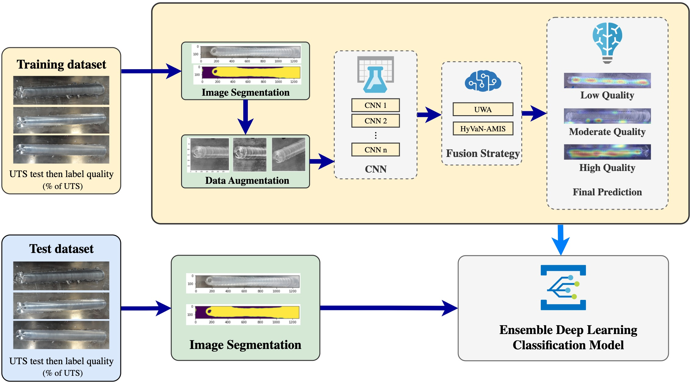
We were unable to uncover research that directly predicts the UTS from the weld seam or a mechanism for classifying the quality of the UTS without harming the weld seam, despite an exhaustive review of previous literature. Due to the advancement of image processing tools and techniques, we believe that the weld seam, which is the direct result of the FSW, should be able to indicate the UTS. In this study, we created a deep learning model to categorize the quality of the welding. Adapted from Mishra [16], this study classifies the quality of welding into three distinct groups. These three groups are characterized by the percentage of the weld seam’s UTS that is less than the base material. These three categories are (1) UTS less than 70%, (2) UTS between 70% and (3) 85%, and UTS greater than 85% of the base material.

However, setting the parameters in FSW can cause errors, and quality can vary. Verifying the quality of FSW can involve huge costs and the damage to the weld during UTS testing. Analyzing a photograph to predict UTS class can save cost and time during the classification of FSW UTS.

Deep learning models [17,18,19,20,21,22,23,24] have recently made significant strides in computer vision, particularly in terms of medical image interpretation, as a result of their ability to automatically learn complicated and advanced characteristics from images. This is due to their propensity to automatically learn complicated visual features. Consequently, a number of studies have used these models to classify histopathological images of breast cancer [17]. Because of their capacity to share information throughout multiple levels inside one deep learning model, convolutional neural networks (CNNs) [25] are extensively employed for image-related tasks. A range of CNN-based architectures have been proposed in recent years; AlexNet [20] was considered one of the first deep CNNs to achieve managerial competency in the 2012 ImageNet Large Scale Visual Recognition Challenge (ILSVRC). Consequently, VGG architecture pioneered the idea of employing deeper networks with smaller convolution layers and ranked second in the 2014 ILSVRC competition. Multiple stacked smaller convolution layers can form an excellent region of interest and are used in newly proposed pre-trained models, including the inception network and residual neural network (ResNet) [18].

Many studies have attempted to predict or improve FSW UTS with welding parameters. Srichok et al. [26] introduced a revamped version of the differential evolution algorithm to determine optimal friction stir welding parameters. Dutta et al. [27] studied the process of gas tungsten arc welding using both conventional regression analysis and neural network-based techniques. They discovered that the performance of ANN was superior to that of regression analysis. Okuyucu et al. [28] investigated the feasibility of using neural networks to determine the mechanical behavior of FSW aluminum plates by evaluating process data such as speed of rotation and welding rate. Mishra [16] studied two supervised machine learning algorithms for predicting the ultimate tensile strength (MPa) and weld joint efficiency of friction stir-welded joints. Several techniques, including thermography processing [29], contour plots of image intensity [30], and support vector machines for image reconstruction and blob detection [31], have been used to detect the failures of FSW.

Given that, to the best of our knowledge, ensemble deep learning has not been utilized to categorize the quality of FSW weld seams, it is possible to evaluate the UTS of weld seams without resorting to destructive testing. Thus, the following contributions are provided by this study:

(1)

An approach outlining the first ensemble deep learning model capable of classifying weld seam quality without destroying the tested material;

(2)

A determination of UTS quality using the proposed model and a single weld seam image;

(3)

A weld seam dataset was created so that an effective UTS prediction model could be designed.

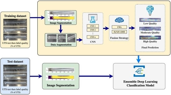
Figure 1 shows a comparison of the proposed method with the traditional weld seam UTS testing method. In the traditional method, the specimen is cut out and then tested with the UTS testing machine, while the proposed model uses an image of the weld seam to determine UTS quality.

The study’s remaining sections are organized as follows. Section 2 addresses comparable research in sentiment feature engineering and classification algorithms. In Section 3, we describe two feature set strategies and offer a framework for ensemble classification. The results of the experiments are presented and analyzed in Section 4. In Section 5, we draw conclusions and suggest research subjects for the future.

2. Related Work

2.1. Friction Stir Welding and Deep Learning

The rotational speed affects the look of FSW welds on plate surfaces. The physical parameters of FSW joints are used directly to measure the microstructural transformation that takes place during FSW. A number of mechanisms alter the strength of materials, including solid solution strengthening, work hardening, precipitation hardening, and microstructural strengthening. This study investigated the effect of welding speed, rotating speed, shoulder diameter, and welded plate thickness on the strength of aluminum-welded joints in order to determine the ideal combination of welding parameters. The FSW process can be regarded of as a form of hot working in which the spinning pin and shoulder [32] impart substantial deformation to the workpiece. When dynamic recrystallization occurs, the original grain structure of the base material is totally destroyed and replaced with an extremely fine, equiaxed grain structure [33].

2.2. CNN Architecture Prediction of FSW UTS

CNNs are a type of ANN that are mainly used to analyze images. Okuyucu et al. [28] conducted a study to examine the applicability of neural networks in assessing the mechanical characteristics of FSW aluminum plates, taking process conditions such as rotation speed and welding speed into consideration. Boldsaikhan et al. [34] developed a CNN to classify welds as having/not having metallurgical defects.

2.3. Image Classification with Deep Learning

Image classification is the process by which a machine studies a photograph to determine the class to which it belongs. Raw data pixels provide the basis for early image classification. This means that computers can separate individual pixels into images. Two images of the same object will appear drastically different. They may have different foundations, focal points, and postures, for instance. This makes it difficult for computers to recognize and identify certain images with precision. Machine learning is one discipline that falls under the umbrella of artificial intelligence, and deep learning is one of such subfields. Thousands of images of various objects are used in deep learning, which recognizes patterns to learn how to categorize them. The goal of deep learning is for a computer to memorize data independently, without being told what to look for by a human.

CNNs are a type of ANN that are mainly used to analyze images. Traditional machine learning suffers from the disadvantage of relying on the laborious process of manually extracting data features; however, by training data features one layer at a time, utilizing multiple convolution layers and pooling layers, this problem can be solved. A CNN that is built on the TensorFlow platform has the ability to construct a neural network model based on the data that are already available, and to make predictions about data that have not yet been collected. This presents a new method for predicting the strength of FSW UTS. Alexnet [20], GoogLeNet [24], ResNet [18] (ResNet18, ResNet50, and ResNet101), Inception-ResNet-v2 [23], SqueezeNet [19], and MobileNet-v2 [22] are examples of the many CNN deep learning models that are publicly available. These network models are known to demonstrate a higher performance in relation to accuracy.

2.4. Ensemble Deep Learning Model

The ensemble technique, which combines the outputs of multiple base classification models to produce a unified result, has become an effective classification strategy for a variety of domains [27,35]. Using the ensemble technique, various researchers have improved the classification accuracy of topical text classification. In the realm of sentiment categorization, however, there are very few comparable publications, and no comprehensive evaluation has been conducted. In [33], distinct classifiers are built by training with distinct sets of features, and then component classifiers are picked and merged according to a number of preset combination criteria. Yang and Jiang [36] invented a unified deep neural network with multi-level features in each hidden layer to predict weld defect types. When working with a smaller dataset, the output of a CNN achieves superior generalization performance.

3. Materials and Methods

This section covers the research methodology used to construct the deep learning model used to differentiate the FSW-UTS of weld seams. Figure 2 displays the procedure used to construct the proposed model.

The dataset must initially be produced, collected, and then classified. The dataset was separated into two groups: the training dataset and the testing dataset. The training dataset was utilized to build a model consisting of four steps: (1) image segmentation, (2) image augmentation, (3) CNN model construction, and (4) decision fusion techniques. Finally, the suggested model was evaluated using the test dataset. Further steps are described below.

3.1. Friction Stir Welds and Weld Seam Dataset

This study used an image dataset based on the materials AA5083 and AA5061, which were prepared according to the American Welding Society standard [37]. Following the completion of the welding operation, tensile testing equipment was used to evaluate the UTS. Photos were taken of the specimens, and UTS was tested until the sample reached breaking point and the UTS was recorded. The UTS measurements were classified according Mishra’s study [38], and each FSW image was labeled. The literature review revealed that these parameters of dissimilar materials in the FSW process include rotation speed, welding speed, shoulder diameter, tilt angle, and pin profile, all of which affect sufficient heat generation, plastic deformation, and material flow in the weld seam [39]. The particle reinforcing additives, such as silicon carbide [40] and aluminum oxide [41], were employed to improve the weld seam’s quality.

Table 1. Details of the parameters used to prepare the dataset.

Continuous Parameter
Parameter		Min	Max
Pin length (mm)		4.8	5.5
Shoulder diameter (mm)		18	25
Pin bottom diameter (mm)		6	8
Tilt angle (°)		0	3
Rotation speed (rpm)		150	1500
Traveling speed (mm/min)		15	135
Penetration (mm)		0.3	0.5
Categorical Parameter
Parameter	Levels
Pin type (cylindrical)	Straight	Hexagonal	Threaded
Additive	Silicon carbide	Aluminum oxide	-
Technique for additive	Drill	Groove	-
Traveling method	Straight	Zig zag	Circles

summarizes the parameters that varied during the experiment in order to obtain various weld seam appearances.

Minitab optimizer was used to calculate the Box–Behnken designs, which are experimental designs for response surface methodology [26]. Each parameter level was picked at random for use with a particular specimen. The experimental FSW image dataset comprises 1664 images [42] obtained through 416 prepared specimens and UTS testing. Wiryolukito and Wijaya [43]’s investigation exercised a fair comparison by employing identical sample sizes for the training set and test set. The dataset was divided into a training set of 82.45% and a test set of 17.5%. The experimental FSW image dataset consists of 1664 data points from the specimen preparation and test for UTS. The sizes of both the training set and the test set were identical to those used in the study by Wiryolukito and Wijaya [43].

Table 2. Characteristics of our proposed dataset.

UTS Range	2 Classes		3 Classes
	<70%	>70%	<70%	70–85%	>85%
	<194.45 MPa	>194.45 MPa	<194.45 MPa	194.45–236.10 MPa	>236.10 MPa
Train set	504	868	504	392	476
Test set	110	182	110	80	102
Total	614	1050	614	472	578

shows the dataset was split into two parts: 82.45% for training, and 17.55% for testing. In addition, the training set was divided such that 80% of it was used for training and 20% was used for validation. Deep learning bi-classification and multi-classification models were applied to the dataset. For deep learning classification modeling, the output of a given dataset is classified based on whether the UTS is less than 70% of the reference value, between 70% and 85% of the reference value, or greater than or equal to 85% of the reference value, according to Mishra [16].

The pre-processing phase occurs prior to data training and testing. In this study, we used top-view alignment images from specimens [44] to simulate the real-world application with four random image techniques [42] for detecting welding defects. Due to the efficacy of training models, scaling the image is a crucial pre-processing step in computer vision. The smaller the image, the better the performance of the model. The original image resolution of 1280 by 900 pixels obtained from the digital camera was scaled, resulting in an image with dimensions of 224 by 224 pixels. Additionally, the final part of this phase is to undertake the hot encoding of labels, as many machine learning algorithms cannot immediately undertake data labeling. The data are labeled as “high quality”, “moderate quality”, or “low quality”. An example of the labeling of the dataset is shown in Figure 3. All input variables and output variables, including those in this algorithm, should be numeric. The labeled data were converted into a numerical label so that the algorithm could comprehend and interpret them.

3.2. Development of the Ensemble Deep Learning Model

In this study, two methods were employed to improve the efficacy of FSW UTS classification. These methodologies are the data preparation technique of current CNN architecture and the decision technique. Each can be elaborated upon as follows.

3.2.1. Image Segmentation

To improve the image quality of the trained dataset, we modified the adaptive thresholding segmentation suggested in [45]. Segmenting a picture with thresholding involves assigning foreground and background values to each pixel based on whether or not its intensity value is above or below a predetermined threshold. In contrast to the static threshold applied to every pixel in an image by a traditional thresholding operator, adaptive thresholding adjusts the threshold on the fly as it moves across the image. A more complex thresholding method can adjust to varying levels of illumination, such as those produced by a skewed lighting gradient or the presence of shadows. Adaptive thresholding accepts a grayscale or color image as input and generates a binary image that represents the segmentation in its most basic form.

A threshold needs to be determined for each image pixel individually. The pixel’s value is considered as background if it falls below a certain threshold, and as foreground otherwise. Finding the threshold can be conducted in two different ways: (1) using the Chow and Kaneko approach [46] or (2) using local thresholding [46]. Each technique is based on the premise that smaller image portions are more amenable to thresholding because they are more likely to contain uniform illumination. In order to select the best threshold for each overlapping section of a picture, Chow and Kaneko use the histogram of the image to perform segmentation. Results from the sub images are interpolated to determine the threshold for each individual pixel. This approach has the downside of being computationally expensive, making it inappropriate for use in real-time settings. Finding the local threshold can also be performed by statistically analyzing the intensity level of each pixel’s immediate neighborhood. Which statistic is most useful is heavily dependent on the quality of the supplied image. One function that is both quick and easy to calculate is the mean of the local intensity distribution. Figure 4 depicts an example of the segmentation technique that was employed in this study.

3.2.2. Data Augmentation

Data augmentation aims to expand the number and diversity of training data through the creation of synthetic datasets. Most likely, the boosted statistics were drawn from a distribution closely mimicking the original distribution. The larger dataset can then represent more exhaustive characteristics. Various forms of data, such as object recognition [47], semantic segmentation, and image classification [48], can be augmented with image data using a variety of techniques.

Only picture alteration is employed in this study. The focus of fundamental image transformation includes picture transformations such as rotation, mirroring, and cropping. Figure 5 displays an example of image enhancement using multiple enhancement techniques, as explained previously.

Mean–variance–softmax–rescale normalization (MVSR normalization), also known as Luce’s choice axiom, is based on four mathematical operations: the data’s mean, variance, softmax, and rescaling, per R. Duncan Luce’s probability theory [49]. The probability of an occurrence of one sample within the same dataset depends on another sample. Typically, the ultimate activation function of multiclass is softmax. In general, standard deviation [50] is used to create a relationship between data points and to quantify the spread or distribution of a dataset relative to its mean. Probability distribution is developed for the output class using artificial neural network (ANN) models [51]. After calculating the normalized input intensity, the dataset could contain fractional values that are both negative and positive. Softmax is utilized to maintain the influence of negative data and nonlinearity.

3.2.3. CNN Architectures

CNN architectures, including MobileNet-v2 [22], DenseNet-121, EfficientNetB1, ResNet101-v2 [18], and InceptionResNet-v2 [23], were utilized and compared in this study, as these network models are known to exhibit superior performance in terms of accuracy compared with other networks with comparable prediction times. To evaluate the performance of online processing, smaller network models were also added. Therefore, we employed five CNN designs that are particularly useful.

MobileNet-v2

MobileNet-v2 is a methodology that was developed by Google [22] and is based on the convolutional neural network (CNN). It has an improved performance as well as enhancements that make it more efficient.

DenseNet-121

DenseNets need fewer parameters than comparable conventional CNNs since duplicate feature maps are not taught. Its layers are quite thin, and they only provide a small number of new feature maps for the database. DenseNets solve this issue since each network layer has immediate access to both the gradients created by the loss function and the original input image. Each successive layer of DenseNet-121 adds one of these 32 extra feature maps to the volume.

EfficientNetB1

Tan and Le [52,53] invented the concept for EfficientNet in order to investigate which values produce the best results for the hyper parameters used in CNN designs. Scaling for width, depth, resolution, and compound scaling are each included in these hyper parameters in their respective forms. In order to assist the manufacture of an informative channel feature that makes use of GAP summation, squeeze-and-excitation (SE) optimization was also included in the bottleneck block of EfficientNet. This was undertaken for the purpose of reducing production time.

ResNet101-v2

The concept of “skip connections”, also known as “quick forward connections”, is utilized by ResNets. It refers to the process of transferring information from earlier levels to deeper layers after ReLU activation has already been performed. The deep residual networks that constitute ResNet101-v2 have been updated and improved. Resnet101 is an architecture that is composed of 101 layers of deep convolutional neural networks. In ResNet101-v2, the convolutional layers apply the convolutional window with a dimension of 3 × 3, and the number of filters increases with the depth of the networks, going from 64 to 2048. In ResNets, there is only ever one max pooling layer, and the pooling size is always 3 × 3. After the first layer, a stride of 2 is always applied.

InceptionResnet-v2

InceptionResnet-v2 is a sub-version of InceptionResnet inspired by the performance of ResNet. InceptionResNet-v2 has a computational cost that is similar to that of Inception-v4.

The training of the CNN models was carried out with the assistance of adaptive moment estimation (ADAM) [54] with a batch size of 16, a maximum epoch of 200, and an initial learning rate of 0.0001. A starting learning rate of 0.0001, which may appear low, was used because in our previous experiments, we discovered that using conventional learning rates of 0.01–0.001% did not result in a convergent output for the given problem. Although this value may seem low, it was chosen because of this experience.

Table 3. Configurations of convolutional deep learning models.

Deep Learning Models	Paraments	Number of Layers	GPU Training (ms/img.)
			2 Classes	3 Classes
MobileNet-v2	2,227,727	105	9.23032	9.33965
DenseNet121	6,955,918	242	10.4876	10.9023
EfficientNetB1	6,517,039	186	11.9927	12.0685
ResNet101-v2	42,535,055	205	13.5612	13.5670
InceptionResnet-v2	54,280,815	449	15.0699	16.5758

outlines the CNN models and their respective configurations that were utilized in the experiments.

CNN Architecture Ensemble Strategy

In this study, two distinct ensemble procedures were employed to construct the CNN ensemble structures. The effectiveness of both the homogenous and heterogenous CNN ensembles was evaluated. Homogeneous ensemble deep learning involves a collection of identical classifiers (CNN architectures) designed to handle a certain issue. For example, if 10 CNN architectures were employed to construct the classification model, these architectures would all be the same type. Each of the 10 components of the heterogeneous ensemble consists of at least two distinct architectural kinds. Figure 6 shows examples of the heterogenous and homogenous ensemble strategies previously explained.

3.3. Decision Fusion Strategy

The decision strategy compiles the conclusions of the event’s classification, reached by a number of different classifiers, into a single conclusion. Multiple classifiers are typically utilized in conjunction with multi-model CNNs in situations where it is difficult to aggregate all CNN outputs. The unweighted average of the outputs of the different base learners in the ensemble was used in the study to fuse decisions [55]. Ensemble techniques can be homogeneous or heterogeneous [35,56]. When referring to an ensemble, the term “homogeneous ensemble” can mean one of two things: (1) an ensemble that combines one base method with at least two distinct configurations or different variants, or (2) an ensemble that combines one base method with one meta ensemble, such as bagging [57], boosting [32], or random sub-space [33]. These two categories of ensembles each make use of a single fundamental technique. We use the word “heterogeneous” to refer to an ensemble that incorporates the usage of at least two different fundamental approaches in its development.

In this study, in addition to the unweighted average decision fusion technique, optimal weight values were calculated utilizing a hybrid version of the variable neighborhood strategy adaptive search (VaNSAS) introduced in [58] and the artificial multiple intelligence system (AMIS) described in [59]. HyVaN-AMIS is the name of this hybrid variation.

The best real value chosen for multiplication with the prediction value of class j from CNN i ($Y_{ij}$) is called the optimal weight. When determining the final weight, UAM will use Equation (1), while HyVaN-AMIS will use Equation (2). After combining the outputs of several CNNs, $V_j$ is the metric used to assign a classification to class j. To put it another way, the weight of CNN I is denoted by the symbol $W_i$. The number of convolutional neural networks (CNNs) included in the ensemble model is denoted by I.

$$V_j=\frac{{\sum }_{i=1}^I{Y}_{ij}}{I}$$

(1)

$$V_j=\sum _{i=1}^I{W}_i{Y}_{ij}$$

(2)

Whichever class j has the greatest value in the variable $V_j$ will be accountable for creating the forecast result. HyVaN-AMIS will be used to find the balance for $W_i$. There are five stages of HyVaN-AMIS used in this study. The procedure begins with (1) the generation of a set of initial tracks (Tr), continues with (2) the selection of an improvement box (IB), and continues further with (3) the execution of IB by all tracks (Tr), (4) the updating of heuristics data, and the repetition of steps (2)–(4) until the termination condition is met. The number of iterations is used as the model’s termination condition in this investigation. Tr has a dimension of D, which is equal to the total number of convolutional neural networks (I). The total amount of Tr that will be built is NP. Here, we see Tr depicted in

Table 4. Example of initial TR when NP = 2, and I and J = 8.

Tr e\Element l	M-1	M-2	M-3	M-4	M-5	M-6	M-7	M-8
Tr-1	0.22	0.29	0.84	0.30	0.72	0.17	0.94	0.47
Tr-2	0.06	0.94	0.78	0.09	0.39	0.52	0.90	0.09

. Let us assume that this model uses five different CNN architectures, has three classes, and NP = 2.

Different decisions over which IB to employ to enhance the current solution are made by each Tr. Using Equation (3), we can see that there is a discernible probability function for deciding which Tr to use. In each iteration, the Tr will use a roulette wheel method to select the IB [60].

$$P_{bt}=\frac{F{N}_{bt-1}+\left(1-F\right)A_{bt-1}+K{U}_{bt-1}}{{\sum }_{b=1}^{B}F{N}_{bt-1}+\left(1-F\right)A_{bt-1}+K{U}_{bt-1}}$$

(3)

$P_{bt}$ represents the probability of occurrence of IB b in iteration t. The scaling factor F is recommended by [59] to be 0.7. For all iterations between t = 1 and t = t − 1, − $A_{bt-1}$ represents the average objective function of all Trs that picked IB b. K is an unchangeable integer and is set to 3 [59]. If this iteration’s best solution is in IB b, then $U_{bt-1}$ will increase by 1. The number of Trs that select IB b from the first iteration to the t − 1 iteration are denoted by $N_{bt-1}$.

There must be recurrent updates to all of these parameters. Tr will utilize the probability function given by Equation (4) to decide which IB to implement in order to improve itself. This study will employ the three improvement boxes shown in Equations (4)–(6), as suggested by [59,60].

$$Z_{elt}=X_{rlt}+Q_{el}\left(X_{rlt}-X_{nlt}\right)$$

(4)

$$Z_{elt}=\{\begin{array}{c}{X}_{elt} if Q_{el}\le CR \\ R_{elt } otherwise \end{array}$$

(5)

$$Z_{elt}=\{\begin{array}{c}{X}_{elt} if Q_{el}\le CR \\ X_{nlt } otherwise \end{array}$$

(6)

The equation in (IB) is the same as the one in [59]. $Z_{elt}$ is the new generated value in the position using IBs. In each iteration, $X_{elt}$ represents the value of the Tr e element l, while r and m are distinct elements of the set of Tr (1 to E) that are not equal to e. $Q_{el}$ is the random number for the position l in Tr e, and $R_{elt }$ is the random number of Tr e, element l, in iteration t, spread out from 0 to 1. The crossover rate (CR) is 0.8 [59]. Values of $W_i$ are connected to those of $X_{elt+1}$, as shown in Equations (7) and (8), and $X_{elt+1}$ is updated using Equation (8) when $f(Z_{elt})$ is the objective function of $Z_{elt}$ and $f\left(X_{elt}\right)$ is the objective function of $X_{elt}.$

The equation in (IB) is the same as the one in [59]. In every iteration, $X_{elt}$ will stand in for the value of the Tr e element l, while r and m will represent the two elements of Tr (from 1 to E) that are not equal to e. The random number $Q_{el}$ for location l in Tr e, and the random number $R_{elt }$ for element l in iteration t are both in the interval [0, 1]. A CR of 0.8 can be attained [59]. As indicated in Equations (7) and (8), when $f(Z_{elt})$ is the objective function $Z_{elt}$ and $f\left(X_{elt}\right)$ is the objective function of $X_{elt}$, then the values of $W_i$ are linked to those of $X_{elt+1}$, and $X_{elt+1}$ is updated using Equation (8).

$$X_{elt+1}=\{\begin{array}{c}{Z}_{elt} if f\left(Z_{elt}\right)\le f\left(X_{elt}\right) and update f\left(X_{elt}\right)=f\left(Z_{elt}\right)\\ X_{elt+1} otherwise \end{array}$$

(7)

$$W_i=X_{eit}\hspace{1em}\hspace{1em}\mathrm{for} \mathrm{all} e \mathrm{and} t.$$

(8)

In this study, we examined two different methods of decision fusion, as well as image segmentation (Seg), augmentation (Aug), and ensemble deep learning with homogenous and heterogeneous ensemble architecture. The experiment was constructed using experimental design, and

Table 5. Design of an experiment to determine the viability of the proposed model.

	Segment		Augmentation		CNN Architecture					Fusion Strategy
	No Seg.	Seg.	No Aug.	Aug.	CNN1	CNN2	CNN3	CNN4	CNN5	UWA	HyVaN-AMIS
1	✓	-	✓	-	✓	-	-	-	-	✓	-
2	✓	-	✓	-	✓	-	-	-	-	-	✓
3	✓	-	✓	-	-	✓	-	-	-	✓	✓
4	✓	-	✓	-	-	✓	-	-	-	-	✓
5	✓	-	✓	-	-	-	✓	-	-	✓	✓
6	✓	-	✓	-	-	-	✓	-	-	-	✓
7	✓	-	✓	-	-	-	-	✓		✓	✓
8	✓	-	✓	-	-	-	-	✓		-	✓
9	✓	-	✓	-	-	-	-	-	✓	✓	✓
10	✓	-	✓	-	-	-	-	-	✓	-	✓
11	✓	-	✓	-	✓	✓	✓	✓	✓	✓	✓
12	✓	-	✓	-	✓	✓	✓	✓	✓	-	✓
13	✓	-	-	✓	✓	-	-	-	-	✓	✓
14	✓	-	-	✓	✓	-	-	-	-	-	✓
15	✓	-	-	✓	-	✓	-	-	-	✓	✓
16	✓	-	-	✓	-	✓	-	-	-	-	✓
17	✓	-	-	✓	-	-	✓	-	-	✓	✓
18	✓	-	-	✓	-	-	✓	-	-	-	✓
19	✓	-	-	✓	-	-	-	✓	-	✓	✓
20	✓	-	-	✓	-	-	-	✓	-	-	✓
21	✓	-	-	✓	-	-	-	-	✓	✓	✓
22	✓	-	-	✓	-	-	-	-	✓	-	✓
23	✓	-	-	✓	✓	✓	✓	✓	✓	✓	✓
24	✓	-	-	✓	✓	✓	✓	✓	✓	-	✓
25	-	✓	✓	-	✓		-	-	-	✓	✓
26	-	✓	✓	-	✓		-	-	-	-	✓
27	-	✓	✓	-	-	✓	-	-	-	✓	✓
28	-	✓	✓	-	-	✓	-	-	-	-	✓
29	-	✓	✓	-	-	-	✓	-	-	✓	✓
30	-	✓	✓	-	-	-	✓	-	-	-	✓
31	-	✓	✓	-	-	-	-	✓	-	✓	✓
32	-	✓	✓	-	-	-	-	✓	-	-	✓
33	-	✓	✓	-	-	-	-	-	✓	✓	✓
34	-	✓	✓	-	-	-	-	-	✓	-	✓
35	-	✓	✓	-	✓	✓	✓	✓	✓	✓	✓
36	-	✓	✓	-	✓	✓	✓	✓	✓	-	✓
37	-	✓	-	✓	✓	-	-	-	-	✓	-
38	-	✓	-	✓	✓	-	-	-	-	-	✓
39	-	✓	-	✓	-	✓	-	-	-	✓	-
40	-	✓	-	✓	-	✓	-	-	-	-	✓
41	-	✓	-	✓	-	-	✓	-	-	✓	-
42	-	✓	-	✓	-	-	✓	-	-	-	✓
43	-	✓	-	✓	-	-	-	✓	-	✓	-
44	-	✓	-	✓	-	-	-	✓	-	-	✓
45	-	✓	-	✓	-	-	-	-	✓	✓	-
46	-	✓	-	✓	-	-	-		✓	-	✓
47	-	✓	-	✓	✓	✓	✓	✓	✓	✓	-
48	-	✓	-	✓	✓	✓	✓	✓	✓	-	✓

Remark: CNN1: MobileNet-v2; CNN2: DenseNet121; CNN3: EfficientNetB1; CNN4: ResNet101-v2; CNN5: ResNet101-v2.

depicts the experimental design of the proposed processes for classifying the quality of the weld seam. Nonetheless, as shown in Table 5, there are 48 distinct tests in this study.

4. Result

The proposed model has been coded in Python with the Keras and TensorFlow frameworks in order to provide a classification and analysis tool. The algorithm was trained on Google Collaboratory, which provides NVIDIA Tesla V100 with 16 GB of RAM. To simulate the proposed model, a computer with 2 Intel Xeon-2.30 GHz CPUs, 52 GB of RAM, and a Tesla K80 GPU (16 GB of GPU RAM) was employed. The experimental design is depicted in Figure 7. The experimental outcome was carried out. The findings of our computational investigation are provided in the following three parts of this section: (1) revealing the best multiclass classification model of the 48 models shown in

Table 6. KPIs of the proposed methods classifying the UTS of the weld seam.

	Accuracy	AUC	F1		Accuracy	AUC	F1
1	0.2623	0.4540	0.2589	25	0.8180	0.8939	0.8205
2	0.3030	0.4999	0.3038	26	0.8538	0.9345	0.8528
3	0.5339	0.6871	0.5152	27	0.8645	0.9206	0.8668
4	0.5758	0.7434	0.5650	28	0.8983	0.9533	0.8963
5	0.5181	0.6231	0.5026	29	0.8948	0.9299	0.8905
6	0.5606	0.6809	0.5559	30	0.9263	0.9614	0.9318
7	0.5151	0.6301	0.5058	31	0.8728	0.9351	0.8809
8	0.5606	0.6809	0.5559	32	0.9114	0.9574	0.9142
9	0.5083	0.7250	0.5065	33	0.8672	0.9299	0.8707
10	0.5606	0.7808	0.5532	34	0.9048	0.9644	0.9021
11	0.5497	0.6719	0.5212	35	0.9074	0.9368	0.9004
12	0.5909	0.7191	0.5741	36	0.9423	0.9687	0.9385
13	0.2913	0.4812	0.2870	37	0.8574	0.9308	0.8574
14	0.3030	0.4999	0.3038	38	0.8836	0.9591	0.8819
15	0.5554	0.7143	0.5374	39	0.8972	0.9557	0.8972
16	0.5758	0.7434	0.5650	40	0.9247	0.9832	0.9243
17	0.5395	0.6520	0.5289	41	0.9316	0.9695	0.9252
18	0.5606	0.6809	0.5559	42	0.9521	0.9908	0.9519
19	0.5386	0.6548	0.5275	43	0.9119	0.9657	0.9138
20	0.5606	0.6809	0.5559	44	0.9349	0.9872	0.9348
21	0.5346	0.7523	0.5286	45	0.9036	0.9696	0.9049
22	0.5606	0.7808	0.5532	46	0.9281	0.9900	0.9279
23	0.5705	0.6935	0.5484	47	0.9391	0.9679	0.9380
24	0.5909	0.7191	0.5741	48	0.9623	0.9917	0.9622

in order to classify the UTS of weld seams, (2) revealing the best binary classification models of the 48 proposed models shown in Table 6, and (3) comparing the proposed models from (1) and (2) with state-of-the-art methods using the homogenous models of MobileNet-v2, DenseNet121, EfficientNetB1, ResNet101-v2, and InceptionResNet-v2, NasNetMobile, EfficientNetV2B1, and EfficientNetV2S in order to position the proposed model among the various types of CNN architectures.

4.1. Performance of the Multiclass Classification

The outcomes of the 48 tests indicated in Table 5 are shown in Table 6. Three forms of performance measurements were used for classifying the UTS of the weld seam: area under the curve (AUC), F1-score (harmonic mean of precision and recall), and accuracy. AUC is a scalar value between 0 and 1 that measures the predicted performance of a classifier. Equations (9)–(11) computed the accuracy, F1-score, and AUC.

$$accuracy=\frac{T{P}_j+T{N}_j}{T{P}_j+T{N}_j+F{P}_j+F{N}_j}$$

(9)

where TP, FP, FN, and TN are True Positive, False Positive, False Negative, and True Negative values assigning a classification to class j, respectively.

$$\mathrm{F}1=2\times \frac{\left(\frac{T{P}_j}{T{P}_j+F{N}_j}\times \frac{T{P}_j}{T{P}_j+F{P}_j}\right)}{\left(\frac{T{P}_j}{T{P}_j+F{N}_j}+\frac{T{P}_j}{T{P}_j+F{P}_j}\right)}$$

(10)

$$AUC=\underset{0}{\overset{1}{{\displaystyle \int }}}p\left(r_j\right)d{r}_j{ }_{ }$$

(11)

where $p\left(r_j\right), d{r}_j$ are the probability that the classifier will pick a positive sample and randomly select a negative sample for class j, respectively.

The proposed model that provides the highest accuracy for the multiclass classification model is identified in experiment 48, which consists of four steps: (1) image segmentation, (2) image augmentation, (3) use of heterogeneous ensemble structure, and (4) the use of HyVaN-AMIS as the decision fusion strategy.

Table 7. The effects of the components contributing to the proposed model.

	Accuracy	AUC	F1
No segmentation	0.5092	0.6645	0.4993
Segmentation	0.9037	0.9561	0.9035
No augmentation	0.6958	0.7992	0.6910
Augmentation	0.7170	0.8214	0.7119
MobileNet-v2	0.5716	0.7067	0.5708
DenseNet121	0.7282	0.8376	0.7209
EfficientNetB1	0.7354	0.8111	0.7303
ResNet101-v2	0.7257	0.8115	0.7236
InceptionResnet-v2	0.7210	0.8616	0.7184
Heterogenous	0.7566	0.8336	0.7446
UWA	0.6910	0.7935	0.6848
HyVaN-AMIS	0.7219	0.8271	0.7181

summarizes the influence of each of the proposed model components.

When compared to a model that does not use image augmentation, image segmentation can enhance the quality of the solution by 39.45%, while image augmentation can improve the quality of the solution by 2.12%. The accuracy provided by the heterogeneous ensemble structure is 6.03% more precise than other approaches. In conclusion, HyVaN-AMIS offers a solution that is 3.09% superior to that of UWA.

According to the findings of this study, five CNN models, namely MobileNet-v2, DenseNet121, EfficientNetB1, ResNet101-v2, and InceptionResnet-v2, were suggested in order to identify the foundation of the CNN model. Using the FSW image dataset, the CNN models were analyzed and evaluated. Figure 8 presents the CNN training and validation accuracy models of MobileNet-v2, DenseNet121, EfficientNetB1, ResNet101-v2, and InceptionResnet-v2.

Figure 8 shows the accuracy curves and loss curves of each training model for training. When it comes to binary classification, the model performs significantly better than with multiclass classification. It has been noticed that the difference between images of low UTS and high UTS is the curvature in the vertebrae of good UTS. However, this difference is not a powerful differentiator, and results in a high rate of inaccuracy when attempting to differentiate between low UTS and high UTS. This is the primary factor that contributes to the accuracy of binary classification being significantly lower than that of multiclass classification.

4.2. Performance of the Binary Classification

Forty-eight experiments (Table 5) were executed for the binary classification model and the results are shown in

Table 8. KPIs of the proposed binary classification model.

	Accuracy	AUC	F1		Accuracy	AUC	F1
1	0.5441	0.5331	0.0683	25	0.8891	0.9124	0.8709
2	0.5990	0.5988	0.1260	26	0.9258	0.9392	0.9034
3	0.7125	0.8087	0.6891	27	0.8815	0.9340	0.8643
4	0.7796	0.8666	0.7501	28	0.9215	0.9775	0.8972
5	0.7514	0.8303	0.6760	29	0.8699	0.9171	0.8515
6	0.8123	0.8856	0.7429	30	0.9180	0.9478	0.8913
7	0.7241	0.8134	0.6274	31	0.8785	0.9094	0.8436
8	0.7809	0.8689	0.6888	32	0.9033	0.9385	0.8783
9	0.7476	0.8199	0.7187	33	0.8833	0.9348	0.8643
10	0.8126	0.8712	0.7793	34	0.9313	0.9736	0.9026
11	0.7809	0.8006	0.7301	35	0.9009	0.9366	0.8956
12	0.8430	0.8643	0.7925	36	0.9402	0.9695	0.9205
13	0.5662	0.5617	0.0923	37	0.9286	0.9453	0.9029
14	0.5990	0.5988	0.1260	38	0.9512	0.9658	0.9291
15	0.7422	0.8294	0.7129	39	0.9212	0.9720	0.9028
16	0.7796	0.8666	0.7501	40	0.9478	0.9910	0.9237
17	0.7792	0.8548	0.7047	41	0.9090	0.9551	0.8895
18	0.8123	0.8856	0.7429	42	0.9384	0.9753	0.9126
19	0.7472	0.8378	0.6506	43	0.9097	0.9461	0.8766
20	0.7809	0.8689	0.6888	44	0.9307	0.9676	0.9051
21	0.7758	0.8401	0.7483	45	0.9230	0.9691	0.9008
22	0.8126	0.8712	0.7793	46	0.9513	0.9967	0.9292
23	0.8037	0.8251	0.7585	47	0.9376	0.9715	0.9257
24	0.8430	0.8643	0.7925	48	0.9724	0.9966	0.9619

.

Experiment 48’s four-stage proposed model offers the maximum accuracy for the multiclass classification model. Image segmentation, image enhancement, a heterogeneous ensemble, and HyVaN-AMIS are used in the decision fusion approach. This process consists of four stages: (1) image segmentation, (2) image augmentation, (3) the utilization of a heterogeneous ensemble structure, and (4) the application of HyVaN-AMIS as the decision fusion approach. Using data from Table 6 and Table 8,

Table 9. The effects of the components contributing to the proposed model.

	Accuracy	AUC	F1
No segmentation	0.7471	0.8027	0.6223
Segmentation	0.9189	0.9563	0.8970
No augmentation	0.8221	0.8688	0.7488
Augmentation	0.8438	0.8903	0.7705
MobileNet-v2	0.7504	0.7569	0.5023
DenseNet121	0.8357	0.9070	0.8113
EfficientNetB1	0.8488	0.9065	0.8014
ResNet101-v2	0.8319	0.8938	0.7699
InceptionResnet-v2	0.8532	0.9096	0.8278
Heterogenous	0.8764	0.9035	0.8454
UWA	0.8128	0.8608	0.7402
HyVaN-AMIS	0.8547	0.8983	0.7792

provides an overview of the implications of the proposed paradigm’s various components. For instance, the accuracy of “no segmentation” in the first row of Table 9 represents the average accuracy of all experiments in Table 5 without image segmentation (experiments 1 to 24), whereas the accuracy of “segmentation” represents the average accuracy of experiments 25 to 48, which is the model with image segmentation. The final 10 models in Table 9 comprise segmented and augmented models. For instance, the accuracy of the “HyVaN-AMIS” row in Table 8 is the mean of all models that used HyVaN-AMIS as the decision fusion approach, including those with and without image segmentation (models 2, 4, 6, 8,…, 48).

Image segmentation can improve the quality of a solution by 17.18% compared to solutions without image segmentation. The accuracy of the model that uses image segmentation is 0.9189, while the average accuracy of the model without image segmentation is 0.7471. This is due to the fact that during image segmentation, the system assigns the foreground and background value to each pixel based on the comparison of its intensity value to a specified threshold. A more advanced thresholding method can adapt to different levels of illumination, such as those caused by an asymmetric lighting gradient or the presence of shadows. This allows the developed system to see images with greater clarity and less noise than when using unmodified images. This allows the model that utilizes image segmentation to be more accurate than those that do not. As previously indicated, References [45,46] support this notion. An image augmentation can increase solution quality by 2.17% compared with models that do not use image augmentation.

The heterogeneous ensemble structure provides accuracy that is 5.21% higher than that of alternative methods. Finally, the answer provided by HyVaN-AMIS is 4.04% better than that proposed by UWA. From these results, it is clear that the created model yields the same result, whether we use a multiclass classification model or a binary classification model. This finding suggests that the proposed model is resistant to changes in classification type. Even if the UTS classification grows to include more than three levels in the future, the model can still be used to categorize weld seam quality. Figure 9 and Figure 10 depict the confusion matrices associated with the categorization.

Using the confusion matrices in Figure 10 for the MobileNet-v2 ensemble model as an example, the low-quality class UTS result shows that the MobileNet-v2 ensemble model correctly identified 80 images (72.72%) of low-quality pictures of weld seams. The proposed ensemble model increased this figure to 100 images (90.90%) for the test dataset. Overall, the target and output class predictions were within a comparable range for all classes and datasets, showing that the reported accuracy is representative of the proposed model’s performance for all UTS weld seam qualities.

4.3. Comparing the Best Proposed Models from (1) and (2) to the State-of-the-Art Methods

In the last experiment, image segmentation, image augmentation, and HyVaN-AMIS were fixed for use in the model. The comparisons between different state-of-the-art techniques and the proposed (heterogenous model) multiclass and binary classification model are shown in

Table 10. Performance metrics of ensemble models with 3-class dataset.

Model	Accuracy	AUC	F1	Time (sec.)
MobileNet-v2	0.8835	0.9591	0.8818	0.01263
DenseNet121	0.9246	0.9831	0.9242	0.01394
EfficientNetB1	0.9349	0.9741	0.9146	0.01324
ResNet101-v2	0.9344	0.9714	0.9088	0.01575
InceptionResnet-v2	0.9280	0.9899	0.9278	0.02636
NASNetMobile	0.7089	0.9245	0.6883	0.02455
EfficientNetV2B1	0.8321	0.9625	0.8344	0.01642
EfficientNetV2S	0.8835	0.9741	0.8845	0.02160
Proposed Model	0.9623	0.9917	0.9622	0.02216

and

Table 11. Performance metrics of ensemble models for binary dataset.

Model	Accuracy	AUC	F1	Time (sec.)
MobileNet-v2	0.9418	0.9638	0.9187	0.0035
DenseNet121	0.9462	0.9995	0.9221	0.0090
EfficientNetB1	0.9520	0.9908	0.9519	0.0088
ResNet101-v2	0.9349	0.9871	0.9348	0.0089
InceptionResnet-v2	0.9538	0.9992	0.9316	0.0184
NASNetMobile	0.9261	0.9797	0.8950	0.0210
EfficientNetV2B1	0.9041	0.9693	0.8640	0.0081
EfficientNetV2S	0.9278	0.9692	0.9009	0.0191
Proposed Model	0.9724	0.9966	0.9619	0.0083

. The proposed model is compared with MobileNet-v2, DenseNet121, EfficientNetB1, ResNet101-v2, InceptionResnet-v2, NasNetMobile, EfficientNetV2B1, and EfficientNetV2S.

5. Discussion

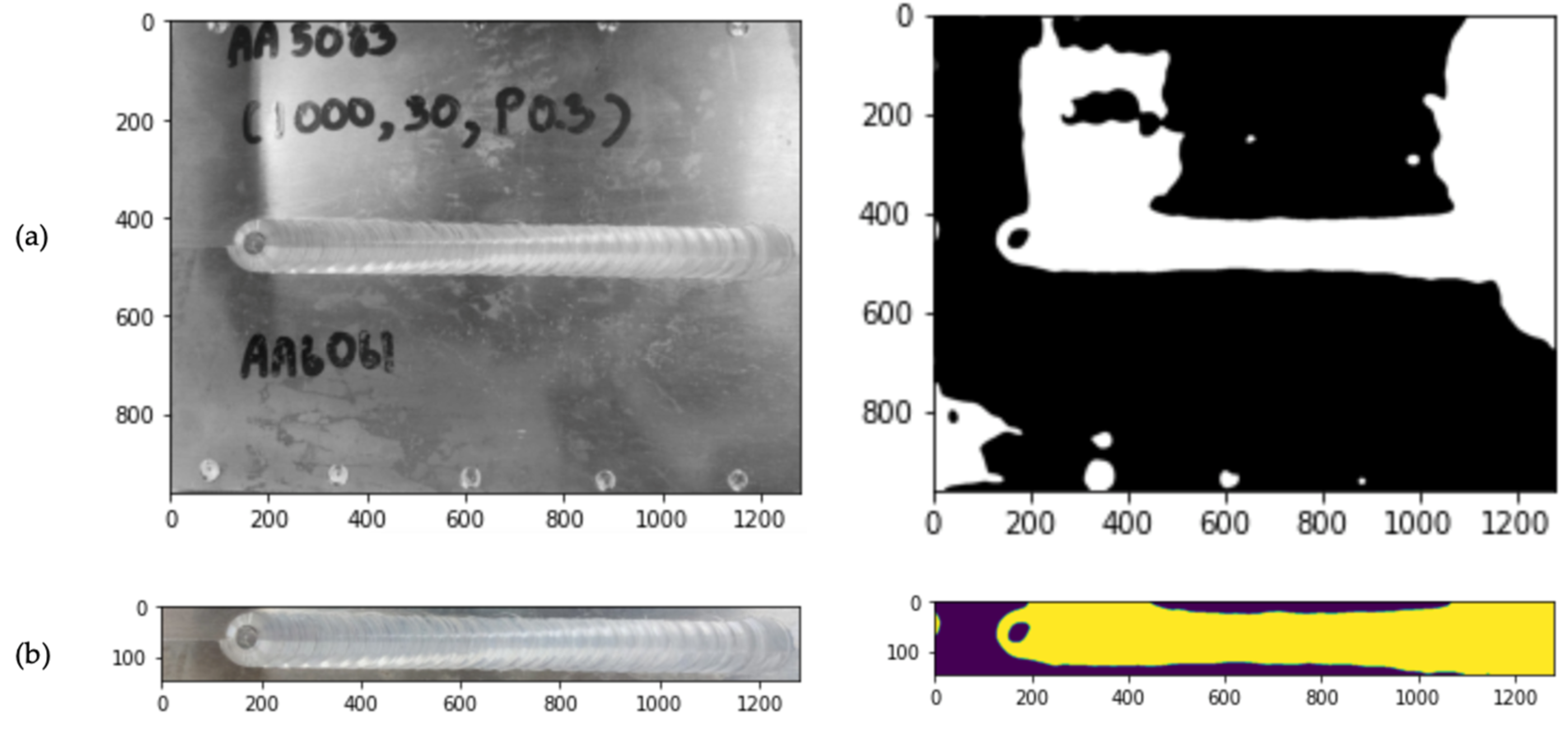
According to Section 4.1 and Section 4.2, the proposed model components contributed to an improvement in classification accuracy. Image segmentation enhances classification accuracy by 17.18% compared to models without image segmentation. The results of [61] indicate that threshold segmentation can improve breast cancer image classification quality. Due to segmentation, the quality of the solution can be enhanced to extract only the essential components for grouping the images into various categories. In spite of this, classification accuracy is improving as a result of a greater emphasis on images’ essential characteristics. Furthermore, this is reinforced by [62,63,64].

Image enhancement is a crucial component that can increase the accuracy of the classification of UTS using a weld seam image. Image augmentation can increase the quality of a solution by 2.17% when compared to a model that does not use it, according to the results presented earlier. This will increase the size of the trained dataset as a consequence of image enhancement. In general, the accuracy of the model will increase as the number of images used to train it grows. This conclusion is supported by [65,66], which demonstrate that image augmentation is an efficient ensemble strategy for improving solution quality.

The image segmentation and augmentation techniques (ISAT) are utilized to de-crease the noise that can occur in classification models. Nevertheless, the application of efficient ISAT would improve the final classification result. As stated previously, the model using ISAT can improve solution quality by 2.17% to 17.18% compared to the model that does not use ISAT. This occurs as a result of the reduction in noise in the image and data structures brought about by these two processes. The robust deblur generative adversarial network (DeblurGAN) was suggested by [67] to improve the quality of target images by eliminating image noise. Numerous types of noise penalties, such as low resolution, Gaussian noise, low contrast, and blur, affect the identification performance, and the computational results demonstrated that the strategy described in this research may improve the accuracy of the target problem. ResNet50-LSTM is a method proposed by Reference [68] for reducing the noise in food photographs, and its results are exceptional when compared to existing state-of-the-art methods. The results of these two studies corroborate our conclusion that the ISAT, which is a noise reduction strategy, can improve the classification model’s quality.

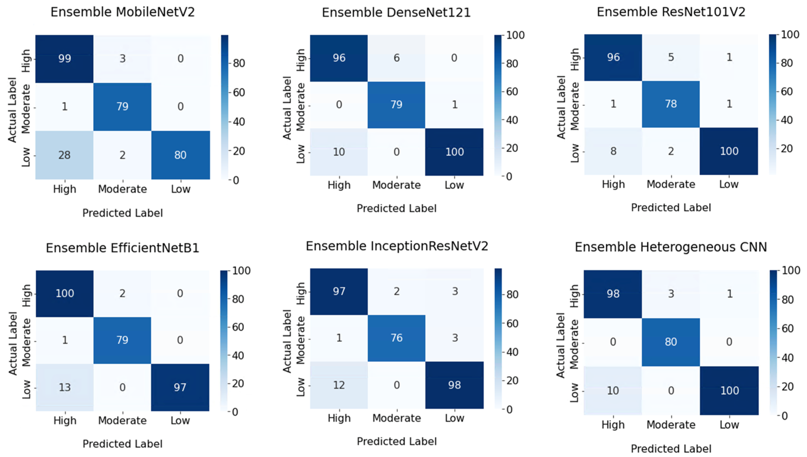
The computational results presented in Table 10 and Table 11 reveal that the heterogeneous ensemble structure of the various CNN designs provides a superior solution to the homogeneous ensemble structures. The classification of the acoustic emission (AE) signal is improved, utilizing a machine learning heterogeneous model as demonstrated in [69]. According to this study’s findings, the heterogeneous model provides a solution that is approximately 5.21% better than the answer supplied by homogeneous structures. This finding is supported by numerous studies, including [70,71,72]. Moreover, Gupta and Bhavsar [73] proposed a similar improvement technique for their human epithelial cell image classification work which achieved an accuracy of 86.03% when tested on fresh large-scale data encompassing 63,000 samples. The fundamental concept behind why heterogeneous structures outperform homogeneous structures is that heterogeneous structures employ the advantages of different CNN architectures to create more effective and robust ensemble models. The weak aspect of a particular CNN architecture can be compensated for, for instance, by other CNN architecture strengths.

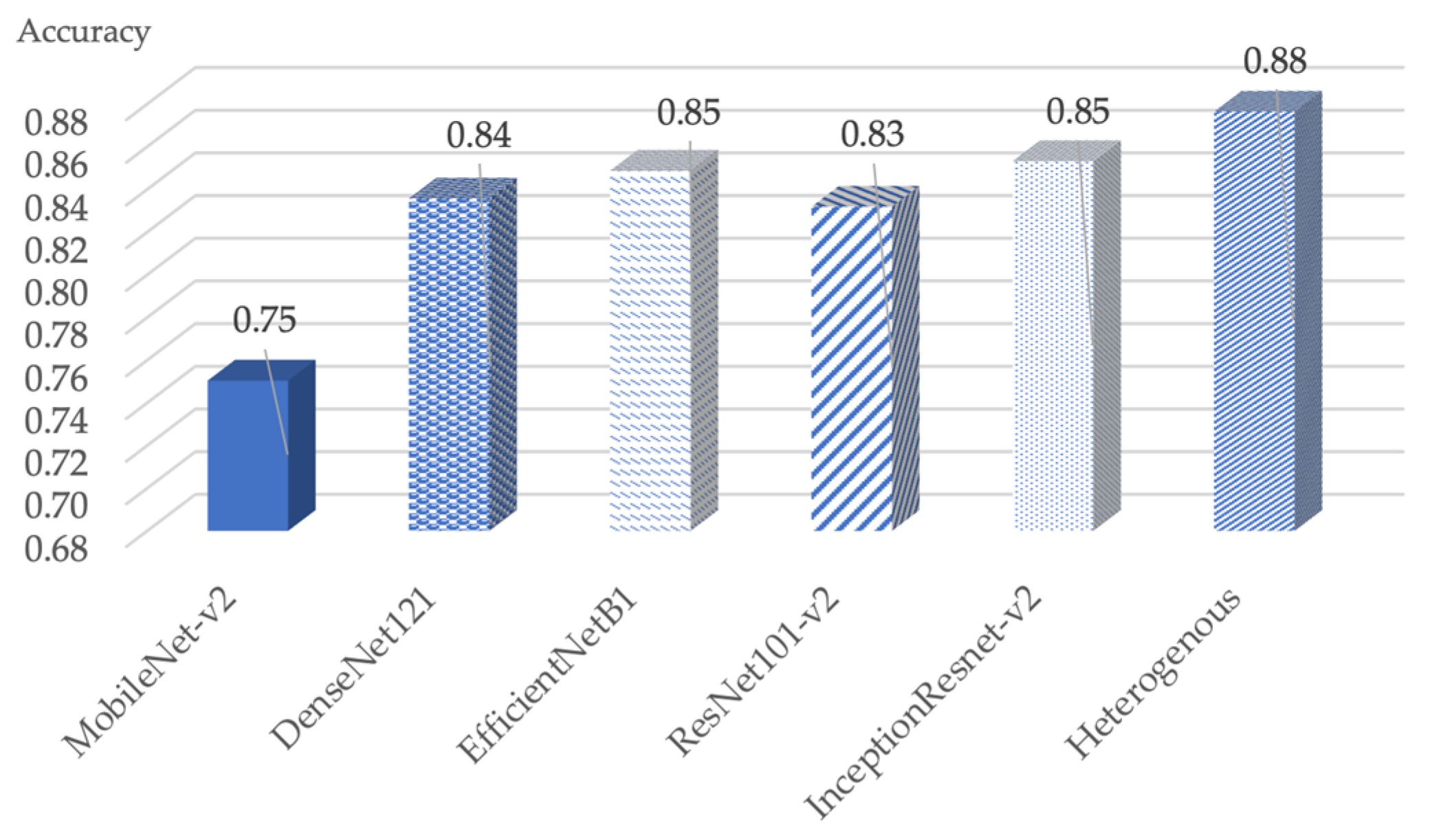
Figure 11 shows the accuracy obtained from various types of CNN architecture, including the heterogenous architectures. The data shown in Figure 11 are taken from in-formation given in Table 9. According to [74], ensemble learning is an essential procedure that provides robustness and greater precision than a single model. In their proposed model, a snapshot ensemble convolutional neural network (CNN) was given. In addition, they suggested the dropCyclic learning rate schedule, which is a step decay to lower the value of the learning rate in each learning epoch. The dropCyclic can lessen the learning rate and locate the new local minimum in the following cycle. The ensemble model makes use of three CNN backbone architectures: MobileNet-V2, VGG16, and VGG19. The results indicate that the dropCyclic classification approach achieved a greater degree of classification precision than other existing methods. The findings of this study validated our research’s conclusion. Using a newly created decision fusion approach, which is one of the most essential procedures for improving classification quality [69], can improve the quality of the answer in comparison to typical fusion techniques.

In this study, the first classification model of UTS based on weld seam outlook is presented. The model given in [38] for predicting the UTS of friction stir welding is based on supervised machine learning regression and classification. The method entails conducting experiments on friction stir welding with varying levels of controlled parameters, including (1) tool traverse speed (mm/min), (2) tool rotational speed (RPM), and (3) axial force. The final result approximates the UTS that will occur when using different levels of (1), (2), and (3), but it is unknown whether the UTS result will be the same when performing FSW welding, which has more than three parameters, and whether the prediction model can be relied upon, despite the fact that the results in the article demonstrate excellent accuracy. Both [75,76] provide a comparable paradigm and methodology.

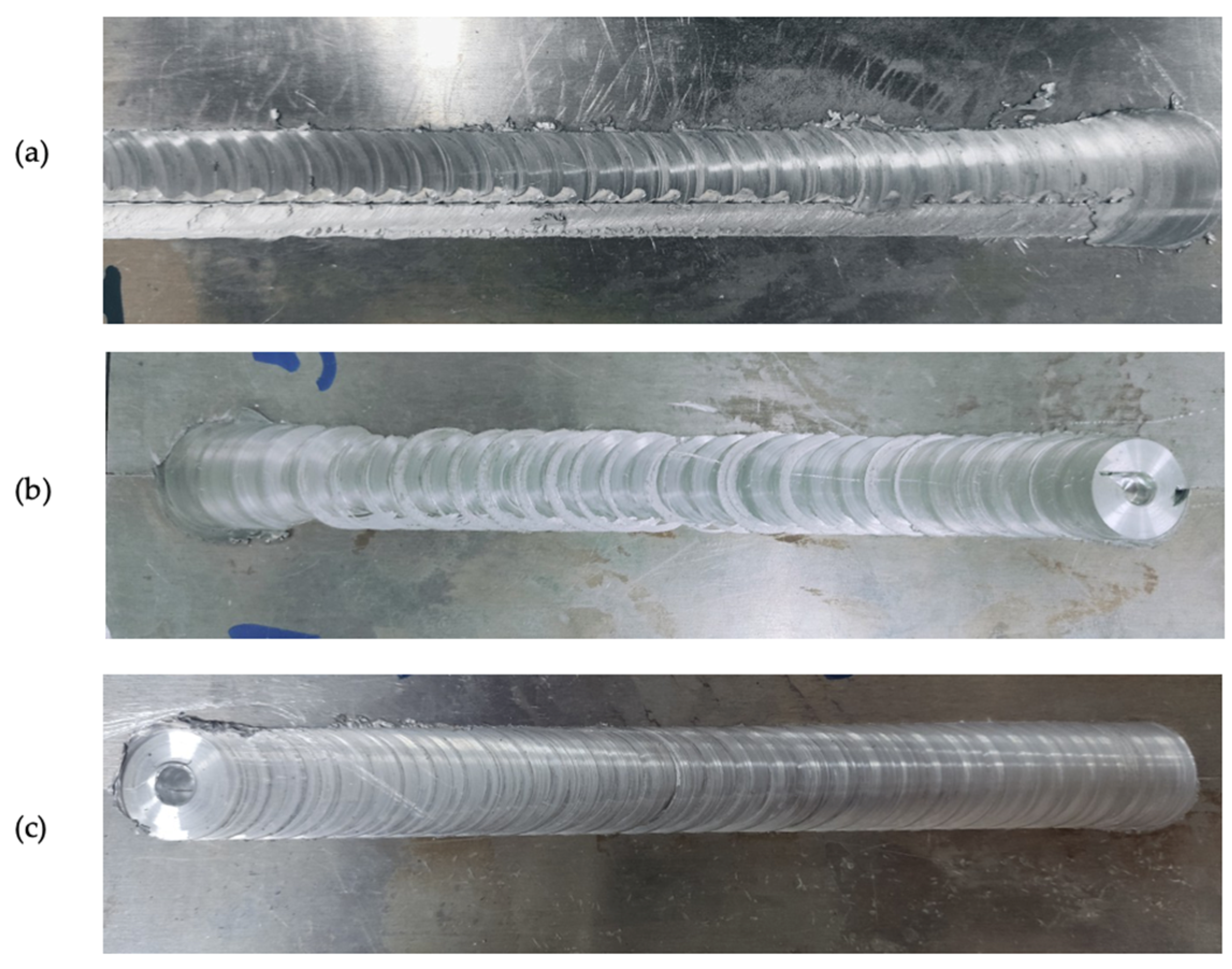
Figure 12 is a GradCam image of a weld seam derived from an experiment with a three-class classification training dataset. GradCam employs the gradients of the classification score relative to the final convolutional feature map to identify the image components that have the largest impact on the classification score. Where this gradient is strongest is where the data influence the final score the most. It is demonstrated that the model will initially evaluate the UTS of the welding joint area (welding line). From Figure 12, the low quality of the weld seam can be identified mostly from the middle of the weld seam in the photograph. If this component exhibits a poor joining appearance, the model will classify it as “low-quality weld seam: low UTS”. For moderate- and high-quality weld seams (high UTS), the model will determine the edge of the weld seam. If it sees an abnormality, then “moderate quality of weld seam” will be assigned to that image, and if it cannot find an abnormal sign, then “high quality of weld seam” will be assigned to that image. It is demonstrated that the classification result of a weld seam image uses several regions to identify which corresponds to the results discussed in [77,78].

In our study, in contrast to the three discussed above, we are not interested in the input parameters, but rather the end outcome of welding. The weld seam is used to determine whether the UTS is of low, moderate, or high grade. The number of parameters and the level of each parameter are no longer essential for classifying welding quality. Due to the fact that the degree of UTS is decided by the base material UTS value, the only thing that matters is which material is using the FSW. This method can be used in real-world welding when FSW has been completed and it is unknown whether the weld quality is satisfactory. The proposed model can provide an answer without destroying any samples.

Table 12. Performance metrics of ensemble models for binary dataset.

No.	PL	SD	PBD	TA	RS	TS	Pe	PT	Ad	TFA	TM	Weld Seam Image	UTS Experiment (MPa)	UTS Prediction (MPa)
1	5.50	25.00	6.00	3.00	865.50	15.00	0.50	SC	SCi	Dr	Str		232.07	194.45–236.10
2	4.80	18.00	6.00	0.00	150.00	15.00	0.50	SC	SCi	Dr	ZZ		135.74	Less than 194.44
3	4.80	18.00	6.00	2.00	150.00	15.00	0.50	TC	SCi	Gr	Str		150.81	Less than 194.44
4	4.80	25.00	8.00	3.00	1500.00	15.00	0.50	SC	AO	Dr	Str		225.70	194.45–236.10
5	5.20	25.00	8.00	3.00	150.00	135.00	0.50	SC	AO	Dr	Cr		145.20	Less than 194.44
6	4.80	18.00	6.00	0.00	1500.00	15.00	0.30	TC	SCi	Dr	Str		246.32	More than 236.10
7	5.50	19.90	7.70	0.00	150.00	135.00	0.30	TC	AO	Dr	Str		165.50	Less than 194.44
8	4.90	18.00	7.20	0.00	1500.00	15.00	0.50	SC	SCi	Gr	Str		197.43	194.45–236.10
9	5.50	25.00	7.60	3.00	1500.00	135.00	0.30	SC	AO	Dr	Cr		201.65	194.45–236.10
10	4.90	18.00	6.60	1.50	1149.00	135.00	0.40	SC	SCi	Gr	Str		237.54	More than 236.10
11	4.80	23.80	6.00	3.00	1500.00	95.40	0.50	TC	SCi	Dr	Cr		210.94	194.45–236.10
12	4.80	25.00	8.00	3.00	150.00	101.40	0.30	SC	AO	Gr	ZZ		118.00	Less than 194.44
13	4.80	18.00	6.00	2.60	1500.00	135.00	0.30	TC	AO	Gr	Cr		231.65	194.45–236.10
14	5.50	25.00	8.00	1.40	1500.00	15.00	0.30	HC	SCi	Dr	Str		239.69	More than 236.10
15	5.50	25.00	8.00	0.00	1297.50	87.00	0.50	HC	AO	Gr	Str		240.34	More than 236.10

Remarks: PL: pin length (mm.); SD: shoulder diameter (mm.); PBD: pin bottom diameter (mm.); TA: tilt angle (degrees); RS: rotation speed (rpm); TS: traveling speed (mm./min); Pe: penetration (mm.); PT: pin type; Ad: additive; TFA: technique for additive; TM: traveling method; WSI: weld seam image; SC: straight cylindrical; TC: threaded cylindrical; HC: hexagonal cylindrical; SCi: silicon carbide; AO: aluminum oxide; Dr: drill; Gr: groove; ZZ: zig zag; Str: straight; Cr: circles.

displays the outcome of the experiment conducted to validate the accuracy of the suggested model submitted to the new experiment. We conducted the experiment by randomly selecting 15 sets of parameters from Table 2. The UTS was then tested using the same procedure as described previously. The weld seam of these 15 specimens has been extracted, and the proposed classification model has been applied to classify the UTS. The outcome demonstrated that 100% of all specimens can be correctly categorized. Six, five, and subsamples were categorized as having UTS values between 194.45 and 236.10 MPa, less than 194.45 MPa, and greater than 236.10 MPa, respectively. The outcome of the actual UTS test matches the classification mode result exactly. This confirms that only weld seams can be used to estimate the UTS of the weld seam. Even though the current model cannot predict exactly (classified within the range of UTS), it serves as an excellent beginning point for research that can predict UTS without destroying the specimen. In the actual working environment of welding, it is impossible to cut the specimen to test for the UTS, and it is nearly impossible to cut the weld seam to test after welding is completed. This research can assist the welder in ensuring that the quality of the weld meets specifications without harming the weld seam.

Table 12 provides evidence that the weld seam outlook can be used to determine the UTS of the FSW. This may be consistent with [79,80]. According to [79], the typical surface appearance of FSW is a succession of partly circular ripples that point toward the beginning of the weld. During traversal, the final sweep of the trailing circumferential edge of the shoulder creates these essentially cycloidal ripples. The distance between ripples is regulated by the tool’s rotational speed and the traverse rate of the workpiece, with the latter increasing as the former decreases. By definition, the combined relative motion is a superior trochoid, which is a cycloid with a high degree of overlap between subsequent revolutions. Under optimal conditions, the surface color of aluminum alloys is often silvery-white. Reference [80] carried out frictional spot-welding of A5052 aluminum using an applied process. The investigation indicated that the molten polyethylene terephthalate (PET) evaporated to produce bubbles around the connecting interface and then cooled to form hollows. The bubbles have two opposing effects: their presence at the joining interface prevents PET from coming into touch with A5052, but bubbles or hollows are crack sources that generate crack courses, hence reducing the joining strength. It therefore follows that the appearance and surface characteristics of the weld seam can reflect the mechanical feature of the FSW that corresponds with our finding.

In addition, the deep learning approach may be utilized to forecast the FSW process parameters backward from the obtained UTS of the classification model. The data obtained in Section 3.1 can be characterized as the parameters found. The UTS can be considered the input, while the collection of parameters is interpreted as the output. Then, these models are utilized to estimate the set of parameters based on the UTS obtained. This is one form of multi-label prediction model. This can correspond to the proposed research in [81]. This research predicts the macroscopic traffic stream variables such as speed and flow of the traffic operation and management in an Intelligent Transportation System (ITS) by using the weather conditions such as fog, precipitation, and snowfall as the input parameters that affect the driver’s visibility, vehicle mobility, and road capacity.

6. Conclusions and Outlook

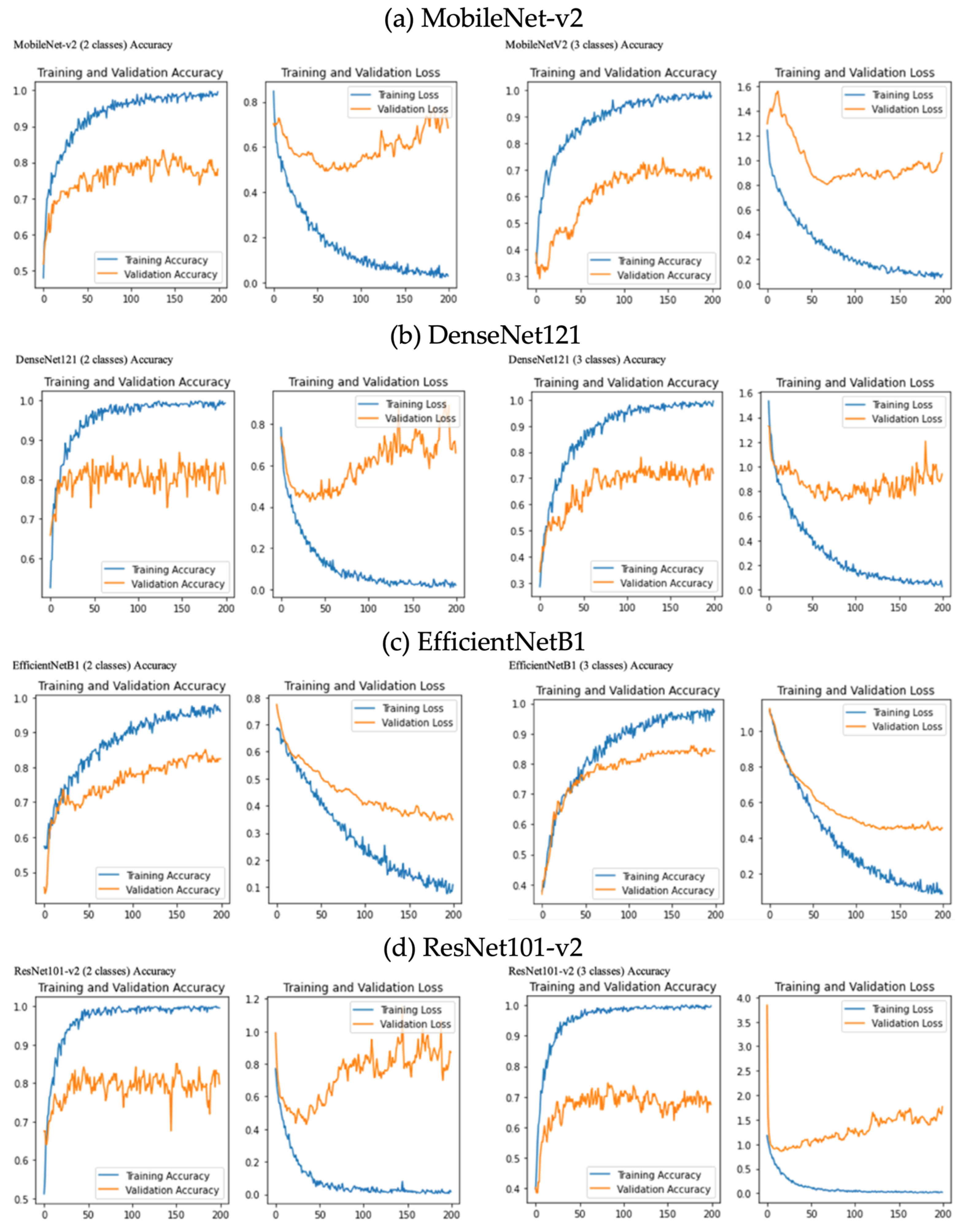
In this study, we developed an ensemble deep learning model with the purpose of distinguishing UTS weld seams from FSW weld seams. We constructed 1664 weld seam images by altering 11 types of input factors in order to obtain a diverse set of weld seam images. An ensemble deep learning model was created to differentiate UTS from the weld seam. The optimal model consisted of four steps: (1) image segmentation, (2) image augmentation, (3) the use of a heterogeneous CNN structure, and (4) the use of HyVaN-AMIS as the decision fusion technique.

The computational results revealed that the suggested model’s overall average accuracy for classifying the UTS of the weld seam was 96.23%, which is relatively high. At this time, we can confidently assert that with our controlled execution of FSW, the weld seam can be utilized to forecast UTS with an accuracy of at least 96.23%. When examining the model in depth, we discovered that image segmentation, image augmentation, the usage of heterogeneous CNN structure, and the use of HyVaN-AMIS improved the quality of the solution by 17.18%, 2.17%, 5.21%, and 4.04%, respectively.

The suggested model is compared to the state-of-the-art method of computer science communication, which is typically used to identify various problems in medical and agricultural images. We adapted these CNN architectures to classify the UTS of the weld seam images, and the computational results demonstrate that the proposed model provides a 0.85% to 7.88% more accurate classification than eight state-of-the-art methods, namely MobileNet-v2, DenseNet121, EfficientNetB1, RessNet101-v2, InceptionResnet-v2, NasNetMobile, EfficientNetV2B1, and EfficientNetV2S.

In order to build a categorization model that is more accurate, it is necessary to construct a classification model that is more precise in future studies. Image segmentation improvement is a procedure that can significantly increase accuracy. Due to the fact that real images from diverse sources with different cameras, light conditions, temperature conditions, and skill of the photographer may result in varied image quality, image segmentation is necessary to future-proof the classification model. In addition, it cannot be assured that the proposed model will continue to show excellent performance when the experiment’s base material is changed; consequently, additional weld seam images from different base materials must be evaluated and incorporated into the model.