Article

Experimental and Numerical Study for Gas Release and Dispersion on Offshore Platforms

1
Engineering Technology Research Institute of Xinjiang Oilfield Company, No. 87, Shengli Road, Karamay 834000, China
2
Centre for Offshore Engineering and Safety Technology, China University of Petroleum (East China), No. 66, Changjiang West Road, Qingdao 266580, China
*
Author to whom correspondence should be addressed.
Processes 2023, 11(12), 3437; https://doi.org/10.3390/pr11123437
Submission received: 16 October 2023 / Revised: 15 November 2023 / Accepted: 19 November 2023 / Published: 15 December 2023
(This article belongs to the Special Issue Risk Assessment and Reliability Engineering of Process Operations)

Abstract

:
Accidental gas release is a major triggering event for the offshore oil and gas industry. This paper focuses on the experimental and numerical investigation for dispersion behavior of released gas on offshore platforms. For this purpose, an experimental system is designed and developed to investigate gas release and dispersion. A series of experiments are carried out, among which the scenarios with constant leakage rates and time-varying leakage rates are both emphasized. The gas concentrations at different sampling points are obtained to study the dispersion behavior and accumulation characteristics of the released gas. Furthermore, a numerical computational fluid dynamics model is established to replicate the experimental scenarios. Good agreement between experimental data and CFD simulation results is observed by calculating a series of statistical performance measures. The developed numerical model is subsequently utilized to investigate a gas release scenario on a practical offshore platform, in which a fully transient leakage rate is adopted considering the response of process protection measures. The developed numerical model could provide support for risk assessment and optimization of contingency plans against gas release accidents in offshore facilities.

1. Introduction

Accidental gas release poses an important threat to the offshore oil and gas industry. In some disastrous accidents, gas release plays an important role, such as the Piper Alpha disaster, the “12.23” sour gas well blowout, the BP Texas City disaster, and the BP Deepwater Horizon explosion, etc. On a typical offshore platform, extensive facilities are arranged in a congested layout. Furthermore, offshore platforms are usually characterized by limited space and insufficient emergency resources. All of these factors make the workers on the offshore platform even more vulnerable to gas release and its cascading effects.
Many studies have concerned accident modeling and risk assessment for gas release accidents in the process industries [1,2,3,4]. Ref. [5] simulated the dispersion behavior and the subsequent explosion consequence of the BP Deepwater Horizon accident. In a study conducted by [6], a risk-based approach is proposed to assess the overall risk of various combustion products in offshore installations. Ref. [7] investigated the fully transient build-up and decay of a flammable gas cloud using time-varying leakage rates in CFD dispersion simulations. Ref. [8] predicted the consequences of accidental releases of hydrogen from forklifts within a full-scale warehouse geometry. Ref. [9] concerns the accidental release and dispersion of liquefied natural gas in a processing facility and analyzed the effect of equipment congestion on dispersion characteristics. All these efforts are beneficial for the assessment and mitigation of unforeseen circumstances. However, an accurate description of the gas profile is the foundation of the above studies. It is therefore essential to track the migration trajectory and to grasp the spatial accumulation characteristics of the released gas.
Many efforts have been made to acquire knowledge of the dispersion behavior and accumulation characteristics of the released gas. To this end, numerous experimental and numerical studies have been carried out. For example, a series of large-scale field experiments have been conducted from the 1970s to the 1990s, such as the Burro experiment, the Maplin Sands experiment, the Thorney Island experiment [10], the Kit Fox experiment [11], and the JIP experiment, etc. In these experiments, the dispersion of heavy gas under a constant leakage rate is of interest. However, large-scale field experiments are known to have high risk, high cost, and poor repeatability. And the experiment regarding the dispersion behavior under a time-varying leakage rate remains almost untouched.
The integral model is also a common method to explore the dispersion behavior of the released gas. A lot of integral models have been developed, such as the Gaussian plume model, the SLAB model, the HEGADAS model, and the DEGADIS model. Some simplified assumptions are conducted in these models, which entails these models are of low accuracy, especially for offshore platforms with intensive facilities. In addition, the integral model is good at predicting gas profiles under a constant leakage rate. This modeling concept is not good at capturing the transient characteristics of the released gas under time-varying leakage rates.
The Computational Fluid Dynamics (CFD) method is increasingly being used to predict the gas profile for various gas release scenarios. An available CFD model is of great importance as it can not only provide credible prediction results but also overcome the disadvantages of the experimental method. However, validation of the computational model against experimental data is crucial. A number of CFD calculations for hydrogen dispersion and subsequent gas explosion have been performed as predictions of representative experiments carried out by the Forschungszentrum Karlsruhe (FZK), and the predictions are in good agreement with observations [12,13]. Ref. [14] demonstrated the accuracy of predictions based on CFD modeling against experimental results for gas releases in an offshore module. Ref. [15] validated the CFD model against hydrogen dispersion experiments. All these efforts are constructive in establishing an available CFD model. However, a constant leakage rate is adopted in these experiments, which is an obvious gap.
The leakage rate is closely related to the pressure inside the equipment during the gas release. In general, the entire release process is divided into two stages by the action of isolation. The pressure inside the equipment remains unchanged before isolation, and thus the leakage rate is constant in this stage. After the action taken to isolation, the leakage rate shows a decreasing trend as the equipment depressurizes. Especially when the gas release occurs in process equipment, the emergency shutdown can provide the isolation function by dividing the process equipment into small sections, thereby reducing the pressure inside the equipment. Therefore, both constant leakage rates and time-varying leakage rates can occur during the gas release process. The leakage rate is very important since it has a direct bearing on the dimension of the gas cloud, and then affects the severity of potential escalation accidents of fire and explosion. Ref. [16] proposed release source and mechanism models for different release scenarios. Ref. [17] conducted the classification of release sources and presented the quantitative model for each release mode. The leakage behavior is of interest in these studies. However, the subsequent dispersion behaviors are not fully investigated. Refs. [6,18,19] emphasized that time-varying leakage rates help to obtain the fully transient flammable gas cloud profiles.
The objective of this paper is to analyze the gas dispersion behavior on the offshore platform under different scenarios using experimental and numerical approaches. Both the constant leakage rate and the time-varying leakage rate are emphasized. For this purpose, an experimental system concerning gas release and dispersion on a small-scale offshore platform is constructed, and the experiments of gas release and dispersion with different leakage rates are carried out. The dispersion behavior and accumulation characteristics of the released gas are carefully analyzed. In addition, a CFD-based model is constructed and the validation of the constructed model is performed based on the experimental results. The validated model is employed to investigate an accident scenario that considers the interference of the emergency shutdown (ESD) system and the blowdown system. Some important parameters, such as the gas dimension and spatial distribution, are obtained. Both the experimental and numerical studies can provide insight into the gas release and guidance for emergency response on offshore platforms. The main innovations of this research are the consideration of gas release scenarios with both constant leakage rate and fully transient leakage rate, and the demonstration of the effectiveness of the constructed numerical model in predicting the dispersion behavior of the released gas.
The structure of the rest of this paper is organized as follows: Section 2 gives a description of the gas leakage and dispersion experiment; Section 3 focuses on the validation of the 3D CFD model; Section 4 devotes to the model application by investigating a typical gas release scenario; Section 5 summarizes the work and gives the conclusions of this paper.

2. Offshore Platform Gas Release and Dispersion Experiments

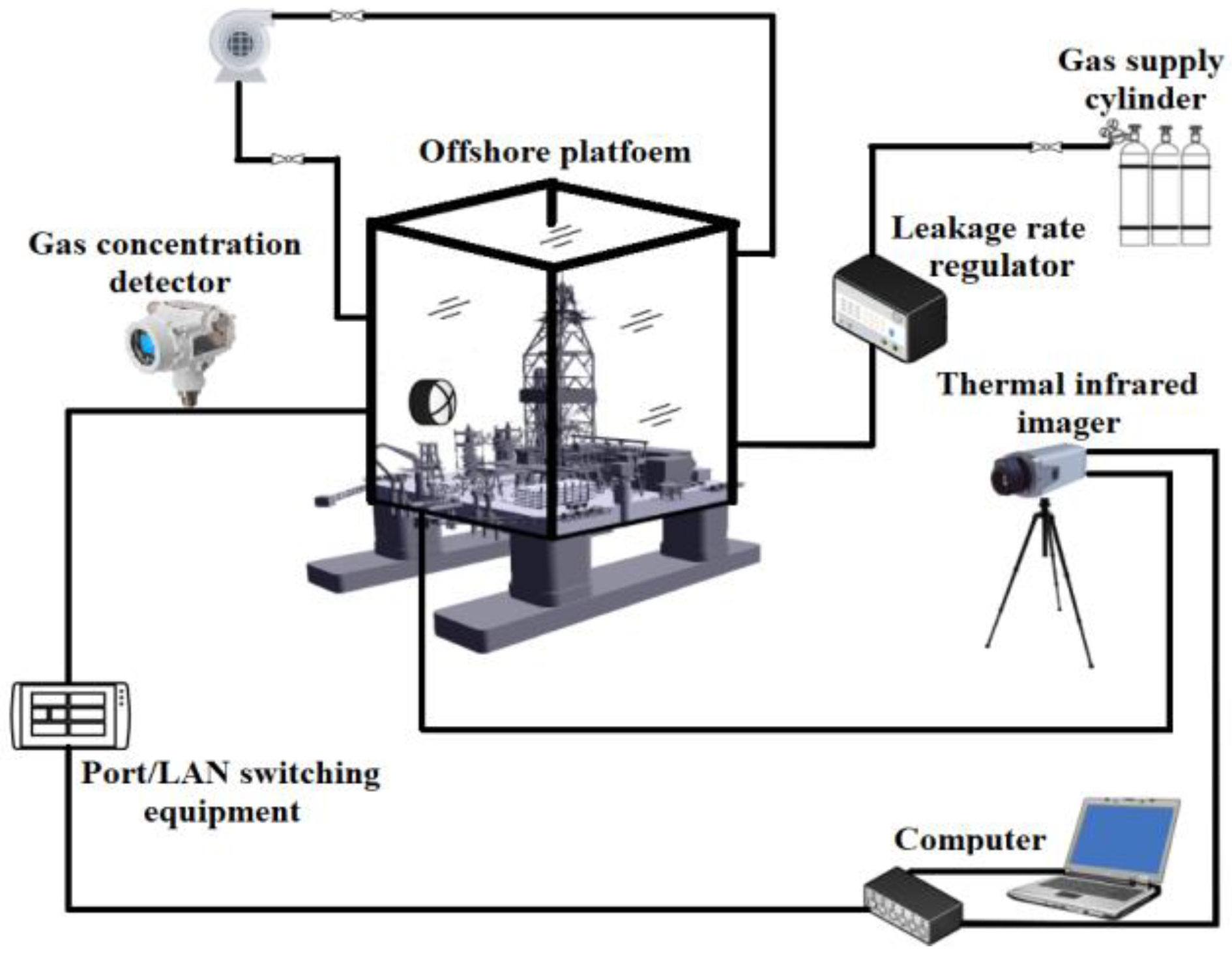
2.1. Experimental Details

As shown in Figure 1, an experimental system concerning the gas release and dispersion on an offshore platform is designed. On the whole, the experimental system includes a gas leakage module, a data acquisition module, and the experimental offshore platform. The gas leakage module serves to obtain the required release rate. The data acquisition module helps to monitor the variation in the gas concentration. The experimental offshore platform (Figure 2) is constructed based on a real offshore platform. The basic dimensions of the experimental offshore platform are summarized in Table 1.

2.1.1. Gas Leakage Module

The gas leakage module consists of a gas cylinder, pressure reducing valve, leakage rate regulator, pressure gauge, temperature gauge, nozzle, and rubber tubing. The released gas is stored in the gas cylinder (Figure 3a). The capacity of the gas cylinder is 8 L. A pressure reducing valve (Figure 3a) is installed at the outlet of the gas cylinder to keep the pressure of the gas flow behind the valve approximately constant. The required experimental pressure could be obtained by adjusting the valve opening. The leakage rate regulator (Figure 3b) is adopted to control and monitor the gas leakage rate. The leakage rate regulator provides manual adjustment function and programmable control function. Both constant leakage rate and time-varying leakage rate are realizable. The pressure gauge and temperature gauges (Figure 3b) are used to monitor the pressure and temperature of the gas flow. The nozzle with an inner diameter of 6 mm is placed on the middle deck of the experimental offshore platform. All of the above devices are connected by rubber tubing. The rubber tubing is 8 m long to reduce the disturbance of the experimenter to the turbulence intensity in the experimental offshore platform. The as-built gas leakage module has the following attributes: (1) the gas leakage module is well sealed and connected to the outside only through the nozzle; (2) the gas leakage rate is adjustable and measurable; (3) the gas release position and direction are adjustable.

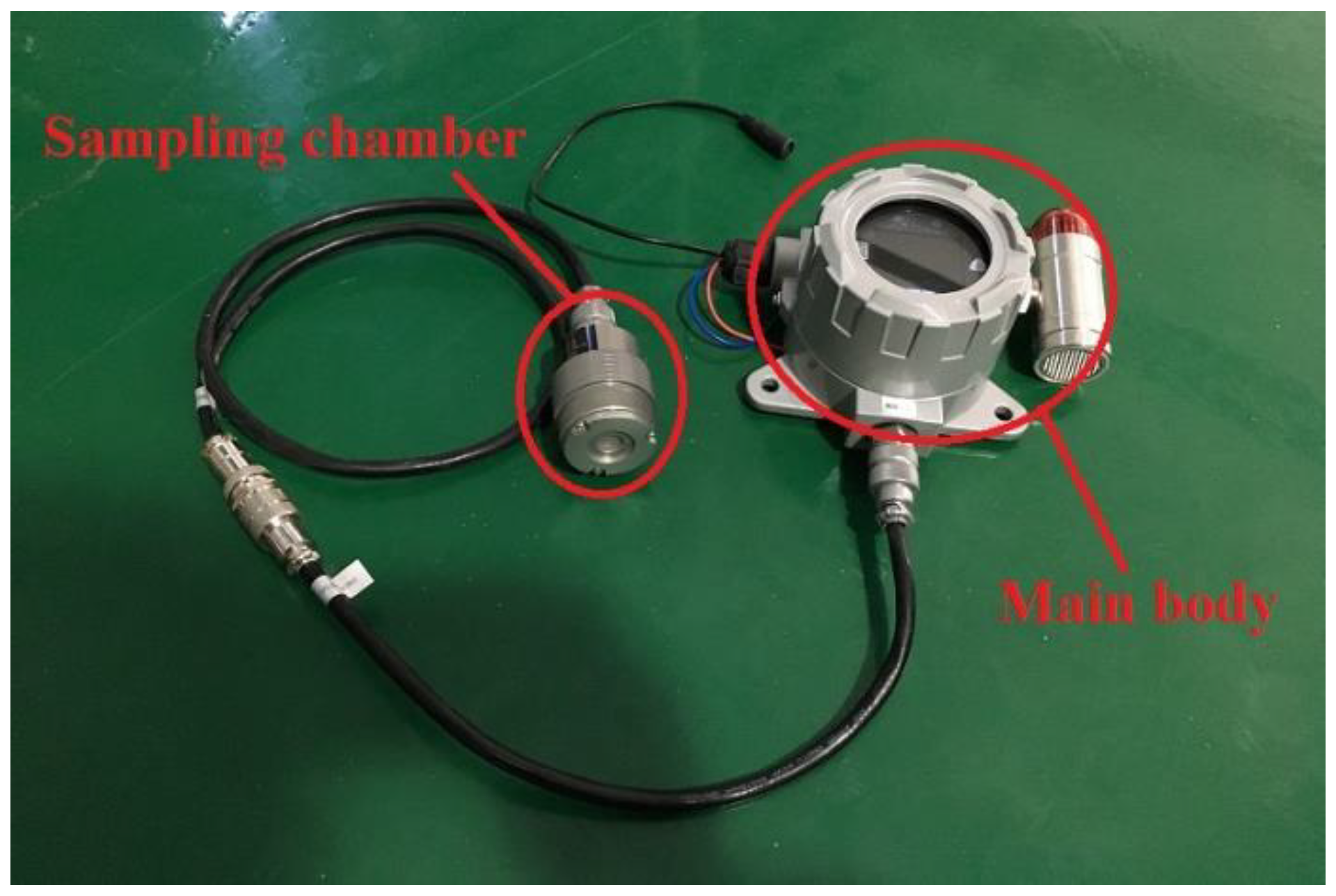
2.1.2. Data Acquisition Module

The data acquisition module mainly includes the gas detector, RS485 communication interface, and PC software. The gas detector is used to analyze the gas concentration. The gas detector adopts the infrared absorption principle. The sampling methods of gas detectors mainly include pump suction sampling and natural dispersion sampling. Pump suction sampling affects the dispersion behavior of the released gas and greatly disturbs the monitoring accuracy, especially for trace gas leakage scenarios. As for natural dispersion sampling, the gas migrates freely into the chamber of gas detectors, which has little effect on the dispersion behavior. Therefore, natural dispersion sampling is exclusively adopted in this data acquisition module. Similarly, the fixed gas detector rather than the portable gas detector is chosen to prevent turbulence intensity from being disturbed. For ease of installation and debugging, the gas detector is customized by separating the sampling chamber from the main body of the gas detector, as shown in Figure 4.
The gas detector can display but cannot store gas concentration data. Therefore, the monitoring data of the gas detector is transmitted to the PC software through the RS-485 communication interface, by which the storage function for the gas detector is bridged. Continuous monitoring and data recording are realized through the data acquisition module. The gas concentration at any moment can be extracted as required.

2.1.3. Other Experimental Details

To meet engineering practice and to avoid interference from inherent gas components (nitrogen, carbon dioxide, etc.) in the air, high purity propane was selected as the released gas in the experiment. The main physical and chemical properties of propane gas are summarized in Table 2. The ambient temperature during the experiment was about 26 °C. Windless is adopted in the experiment.
A total of five gas detectors are arranged in this experimental system. All these gas detectors are also placed on the middle deck of the experimental offshore platform. The gas distribution at a distance from its source is of great significance. Prior to the formal experiments, a series of preliminary experiments were conducted to determine the layout of the gas detectors. A relatively reasonable detector layout was obtained to obtain the gas distribution in the near and far fields. The layout of the gas detectors is illustrated in Figure 5. The nozzle is arranged at the coordinate (50, 100). The gas release direction is horizontal-right. Monitors #1, #2, and #3 are arranged along the gas release direction. The distance between monitor #1 and monitor #2 is 0.14 m, and the distance between monitor #2 and monitor #3 is 0.32 m. Monitor #4 and monitor #5 are offset from the gas release axis. The distance between monitor #4 and monitor #5 is 0.2 m.
During each experiment, the data acquisition module is activated when the gas release is initiated. And the initiation time of gas release is regarded as the starting time of each experiment. Both the sampling and gas concentration analysis are continuous. The gas concentration data is recorded once per second. To reduce the experimental error, the experiment is repeated three times for each scenario, and the final value of the gas concentration is obtained by averaging the results of all the trials.

2.2. Experimental Results and Discussions

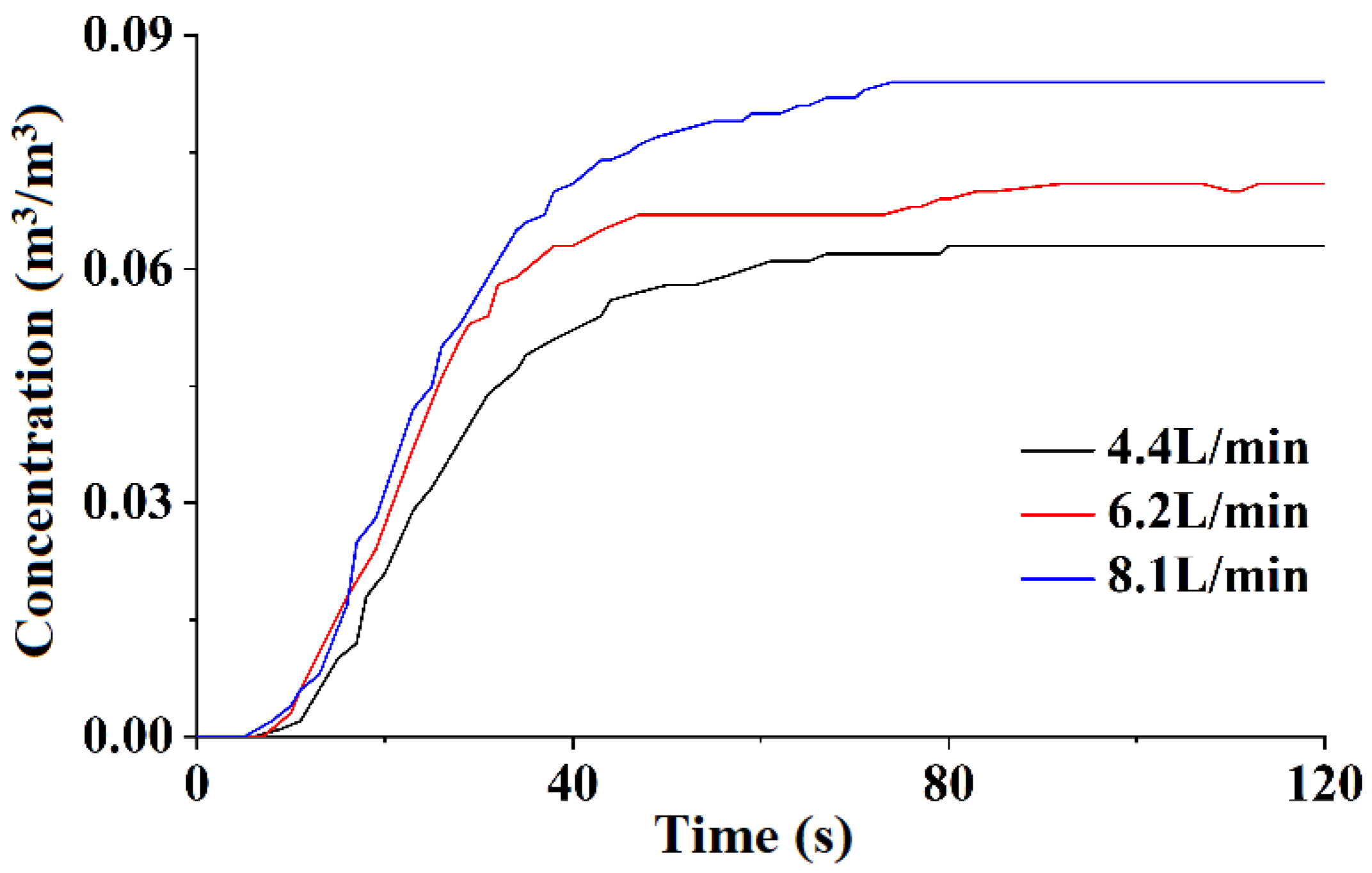
2.2.1. Constant Leakage Rates

A total of three constant leakage rates, including 4.4 L/min, 6.2 L/min, and 8.1 L/min, are considered to discuss the dispersion behavior of the released gas. Figure 6 presents the transient gas concentration at monitor # 1 under different leakage rates. As can be seen, the released gas is detected about 7 s after the gas leakage in different scenarios. The gas concentration increases continuously and then reaches a preliminary stable state. The gas concentration then increases slightly and finally stabilizes due to the sedimentation of propane gas. The steady-state gas concentrations in different scenarios, from big to small, are 8.4%, 6.8%, and 6.3%, respectively. Obviously, the maximum concentration increases as the leakage rate increases. This phenomenon is attributed to the fact that the dilution performance is limited by the leakage rate, and the dilution performance becomes worse with the increase in the leakage rate.
Figure 7 illustrates the gas concentration at different distances along the leakage direction when the leakage rate is 8.1 L/min. As can be seen, the gas concentration at different distances shows a trend of first increasing and then stabilizing. The time for the gas concentration at monitor # 1 and monitor # 2 to reach the stable state is 74 s and 88 s, and the gas concentration in the stable state is about 8.4% and 5.0%, respectively. It can be seen that the gas concentration decreases as the dispersion distance increases, and the time for the gas concentration to reach a stable state increases with the increase in dispersion distance. And monitor #1 detected the released gas earlier than monitor #2. The distance between monitor #1 and monitor #2 is 0.22 m. If the gas leakage rate is 8.1 L/min, i.e., 4.82 m/s, monitor #1 and monitor #2 should detect leakage gas almost simultaneously. However, there is an obvious difference in the time of gas detection for monitor #1 and monitor #2. The phenomena are attributed to pressure loss in the rubber pipeline at the initial stage of gas leakage, resulting in the actual gas leakage rate being smaller than the preset leakage rate at this stage. In addition, the gas is mixed with air in the rubber tubing at the initial stage so that the pure gas is diluted before it enters the atmosphere.

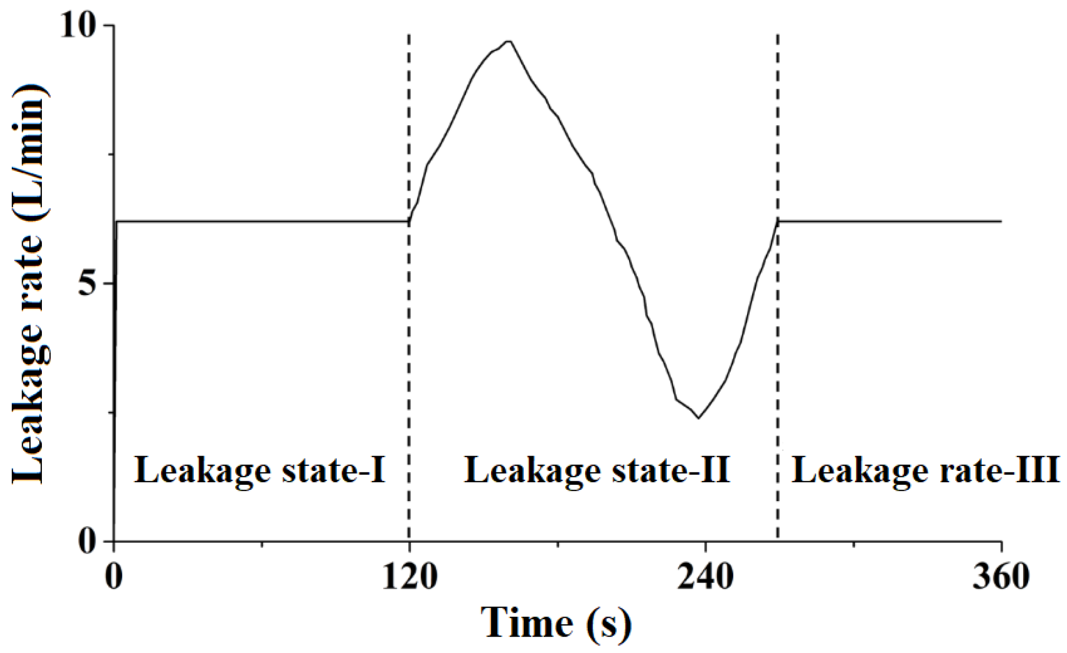
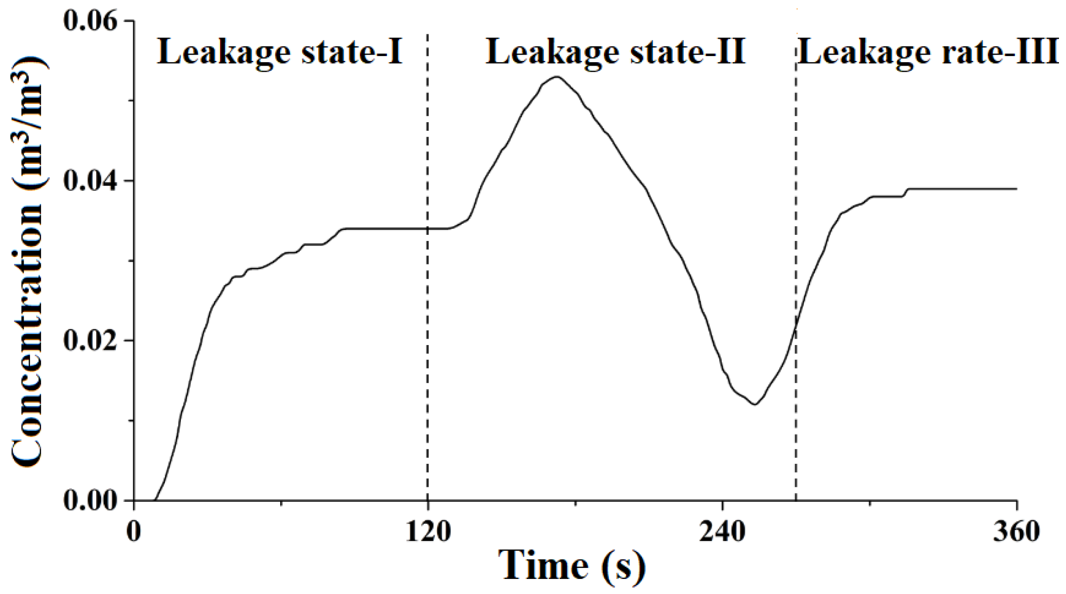
2.2.2. Time-Varying Leakage Rate

This section deals with the gas release scenario with a time-varying leakage rate. As can be seen from experiments with constant leakage rates, both the leakage rate and the gas concentration are lower than the set value in the initial stage. Therefore, a constant leakage rate of 120 s is thereby set in the initial stage. The leakage rate is then set to be time-varying by adjusting the leakage rate regulator. Figure 8 presents the fully transient leakage rate adopted in this section. Overall, the leakage process lasts for 360 s. During 0–120 s, the leakage rate remains constant at 6.2 L/min, and this process is defined as leakage stage I. During 120–270 s, the leakage rate is time-varying, and this process is defined as leakage stage II. The occurrence time of the extremum of the leakage rate is 159 s and 237 s, respectively. The 270–360 s is leakage stage III, and the leakage rate remains constant at 6.2 L/min in this stage.
Figure 9 illustrates the variation in gas concentration at monitor #2 against the transient leakage rate. In leakage state I, the gas concentration at monitor #2 first increases and then stabilizes, showing the same trend as the gas concentration variation against constant leakage rates. In this leakage state, the maximum gas concentration at monitor #2 is 3.4%. In leakage state II, the gas concentration at monitor #2 is also time-varying, and a trend similar to the leakage rate is observed. The extremums of gas concentration during leakage state II are 5.3% and 1.1%, and the corresponding occurrence times are 172 s and 252 s, respectively. In the leakage state III, the gas concentration at monitor #2 reached a stable state after a short rise. Furthermore, it is interesting to find that the gas concentration in leakage state III is higher than that in leakage state I, although the leakage rate in these two states is consistent. The reason for this phenomenon may be that the released gas settles during dispersion and migration. There are also differences in the occurrence time of gas concentration extremums and leakage rate extremums, which is due to the time consumed on gas sampling and concentration measurement.

3. Model Verification

3.1. The Modeling Concept

The gas dispersion satisfies the basic governing equations, including mass conservation, momentum conservation, energy conservation, etc. All these basic governing equations can be represented as [20]:
t ( ρ φ ) + x j ( ρ u i φ ) x j ( ρ Γ φ φ x j ) = S φ
where φ represents the general variable, including mass, momentum, energy, and so on; ρ represents the gas mixture density; t represents time; ui represents the velocity component in i-direction; Гϕ represents the dispersion coefficient of the general variable φ; Sφ represents the source term.
Although models based on large eddy simulations (LES) have gained increasing popularity in recent years, turbulence models based on the Reynolds-averaged Navier-Stokes (RANS) equations are dominant in industrial applications. The RANS equations are closed by invoking the standard k-ε model for turbulence. The standard k-ε model is an eddy viscosity model that tackles the transport equations for turbulent kinetic energy and dissipation of turbulent kinetic energy:
t ( β v ρ k ) + x j ( β j ρ u j k ) = x j ( β j μ e f f σ k k x j ) + β v P k β v ρ ε
t ( β v ρ ε ) + x j ( β j ρ u j ε ) = x j ( β j μ e f f σ ε ε x j ) + β v P ε C 2 ε β v ρ ε 2 k
where βv represents volume porosity; k represents the turbulent kinetic energy; βj represents area porosity in the j-direction; ε represents the turbulent kinetic energy dissipation rate; Pk and Pε represent the production of turbulent kinetic energy and the production of dissipation, respectively; σk and σε represent the Prandtl–Schmidt number of k and ε; C2ε is a constant.
The means of time-average is conducted to describe the instantaneous turbulence in models based on RANS equations. Inevitably, a new variable (i.e., Reynolds stress tensor) is generated, which can be represented as:
σ i j = μ e f f ( u i x j + u j x i ) 2 3 δ i j ( ρ k + μ e f f u k x k )
where σij represents the stress tensor; δij represents the Kronecker delta function, δij = 1 if i = j, δij =0 if i ≠ j.
According to the Boussinesq eddy viscosity assumption, the Reynolds stress tensor is proportional to the strain rate of average velocity. Therefore, an eddy viscosity models the Reynolds stress tensor as follows:
ρ u i u j ¯ = u e f f ( u i x j + u j x i ) 2 3 ρ k δ i j
The μeff in the above equations represents the effective viscosity, which is defined as follows:
μ e f f = μ + ρ C μ k 2 ε
where μ represents dynamic viscosity; the second term is known as the eddy viscosity, and Cμ is a constant.

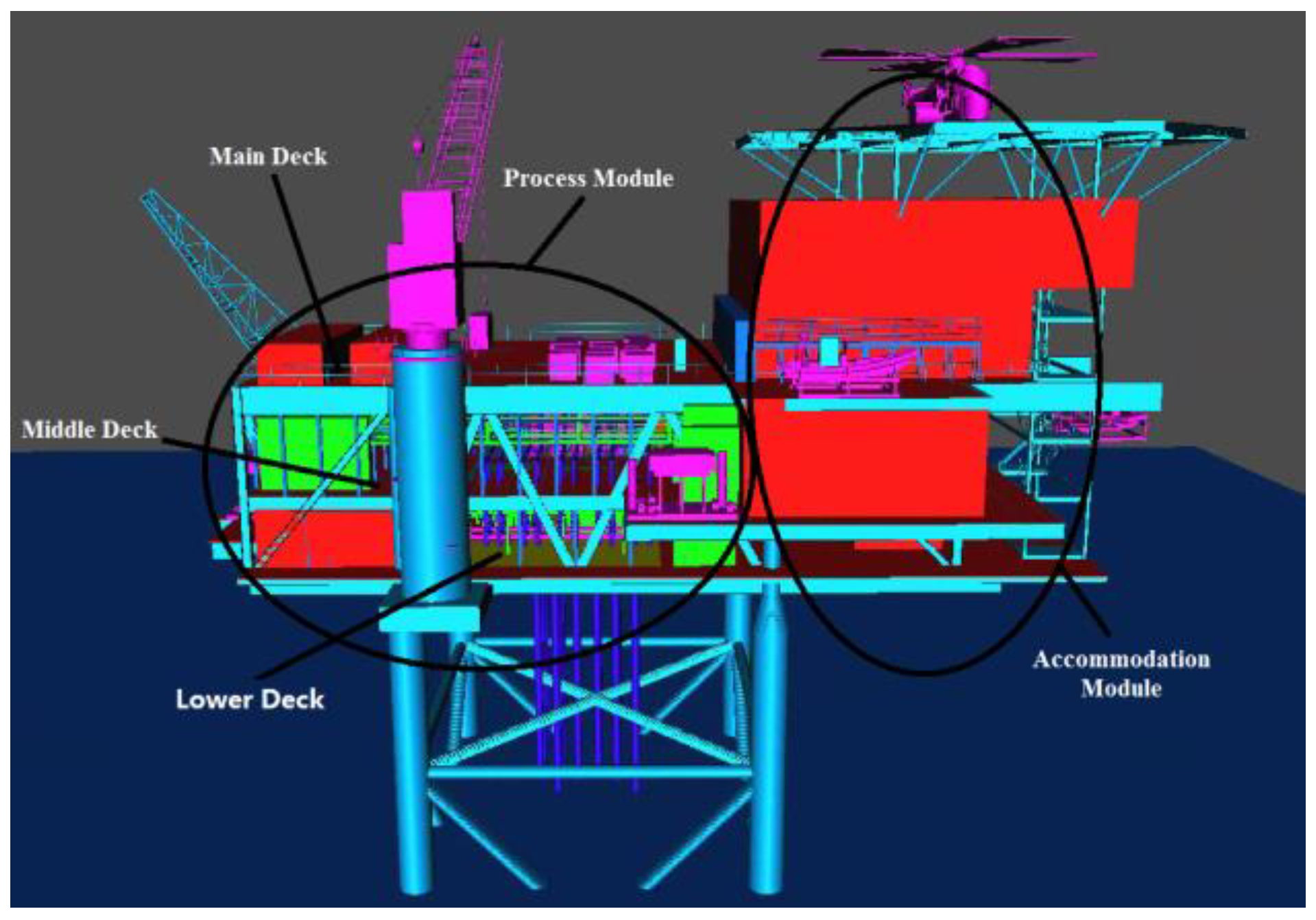
3.2. Geometric Model and Mesh Generation of an Offshore Platform

The experimental scenarios are expected to be replicated by the numerical model. The dispersion of the released gas is affected by the obstacles and thereby it is of great importance to reproduce the geometric features as accurately as possible. A good description of the geometric model is one of the key elements in the numerical calculation. Therefore, a 1:1 geometric model is established based on the target offshore platform. Every geometric detail is taken into account to ensure consistency between the experiment and the numerical calculation. The final as-built 3D geometric model of the offshore platform is illustrated in Figure 10.
The FLACS user manual mainly focuses on numerical calculations involving large-scale geometric models. Accordingly, a meshing method of dividing blocks is recommended, i.e., the computational domain is divided into the core area and the expanding area. The recommended meshing method is not applied in this study considering that the dimension of the geometric model is relatively small. Instead, a uniform grid model is adopted. To balance computational effort and accuracy, grid sensitivity analysis is required. FLAM, a generic parameter describing the Equivalent Stoichiometric Cloud (ESC), is utilized to derive the appropriate grid size. Figure 11 illustrates the variation in FLAM with time under different grid sizes. The computation time and the Max. FLAM under different grid sizes are summarized in Table 3. As can be seen, the FLAM presents a similar trend under different grid sizes. The Max. FLAM decreases as the grid size decreases, and the computation time increases as the grid size decreases. And the Max. FLAM converges with decreasing grid size. The Max. FLAM based on a 0.15 m grid size is very different from those based on other grid sizes. As the grid size increases from 0.1 m to 0.12 m, the Max. FLAM increases by 4.64% while the computation time decreases by 16.76%. When the grid size is reduced from 0.1 m to 0.075 m, there is a small difference of 1.28% for Max. FLAM, while a significant increase of 90.78% is observed for the computational time. Finally, the grid size of 0.1 m is adopted for the subsequent numerical calculation. In addition, local grid refinement around the leak is performed to ensure the stability and accuracy of the numerical computation.

3.3. Basis of Validation of Numerical Calculation Results

The purpose of model verification is to demonstrate that the model is capable of accurately predicting the dispersion behavior of the released gas. A comparison between the numerical calculation results and the experimental results should be conducted to carry out model verification. Therefore, reliable evaluation criteria are essential to identify whether the proposed model can reproduce “reality” to an acceptable degree. In this context, the model evaluation protocol (MEP) provides a constructive reference to determine the evaluation criteria of the quantitative model. A set of statistical performance measures (SPMs) is employed to quantitatively evaluate the effectiveness of the numerical model. The purpose of the SPMs is to provide a measure of the bias and of the spread in the numerical prediction. The SPMs adopted in this study include error, mean relative deviation (MRB), mean relative square error (MRSE), factor-of-2 fraction (FAC2), geometric mean bias (MG), and geometric variance (VG). The acceptance criteria for SPMs are summarized in Table 4. The SPMs can be calculated by:
MRB = C m C p / 0 . 5 ( C p + C m )
MRSE = ( C p C m ) 2 / 0.25 ( C p + C m ) 2
FAC 2 = C p / C m
MG = exp ln ( C m / C p )
VG = exp [ ln ( C m / C p ) ] 2
where Cm represents the experimental data of concentration and Cp represents the model prediction data of concentration.
A lot of physical parameters are available candidates to evaluate a model’s performance. Among them, the representative physical parameters are the gas concentration and the downwind distance to the lower flammable limit (LFL). Ref. [15] argued that gas concentration is the most widely used physical parameter. This viewpoint makes sense because it is difficult to measure the distance to the LFL directly. In practice, the distance to LFL is usually derived by interpolation, which reduces the reliability of this parameter. Therefore, the gas concentration is exclusively adopted to evaluate the performance of the constructed model in this paper.

3.4. Model Validation against Scenarios with Constant Leakage Rates

In the experiment, the sampling area of the gas detector has a diameter of approximately 6 mm. The monitor is associated with an exact coordinate in the numerical simulation. Therefore, a matrix of monitors is set up within the sampling area of the gas detector in the numerical simulation. And the average value of each monitor matrix is utilized to demonstrate the correlation between the experimental results and the numerical simulation results. The monitors with the same coordinates are utilized to demonstrate the correlation between the experimental results and the numerical simulation results. Figure 12 presents the variation in the gas concentration during the experiment and the numerical simulation. As can be seen, a similar trend of first increasing and then stabilizing is also observed in the numerical simulation. The differences are that the released gas is detected in a very short time, and the time required to reach stability is dramatically reduced in the numerical simulation. The differences between them are mainly embodied as follows:
(1) There are differences in the initial period between the experiment and the simulation. Both numerical simulation and experiment take the initiation time of gas release as the starting time. In the numerical simulation, the gas is released immediately at the starting time. In the experiment, however, the gas has to pass through the rubber tubing before it reaches the nozzle. (2) As mentioned above, there is pressure loss and dilution as the gas passes through the rubber tubing. There is a time lag before the gas reaches the designed leakage rate and concentration in the experiment. In the numerical simulation, the pure gas is continuously discharged at the designed leakage rate. (3) Gas sampling takes longer in the experiment. Natural dispersion sampling is adopted in the experiment instead of pump suction sampling. Although natural dispersion sampling helps to obtain more accurate experimental results, it is an inefficient sampling method. In the numerical simulation, gas sampling is defaulted to take no time. (4) The gas detector takes some time to measure the gas concentration in the experiment. The gas detector cannot detect and display the gas concentration in real time. The delay is inevitable no matter what type of gas detector is adopted. On the other side, although the numerical simulation also takes time to analyze the gas, the gas concentration is displayed in real time.
Through the above analysis, it is reconfirmed that there are deviations in the leakage rate and gas purity in the initial period between the experiment and the numerical simulation. Therefore, the gas profiles under a relatively stable state are extracted to discuss the effectiveness of FLACS against experimental scenarios with constant leakage rates.
The SPMs of the numerical simulation results are calculated by taking the experimental results as the benchmark, which are summarized in Table 5. As can be seen, the SPMs meet the acceptance criteria, i.e., the numerical simulation results are in reasonable agreement with the experimental results. In brief, the effectiveness of FLACS on simulation is verified against experimental scenarios with constant leakage rates.
Although a reasonable agreement is observed in each experiment, there are differences between the experimental results and the numerical simulation results, even after the released gas reaches a stable state. The main causes are analyzed and summarized as follows:
(1)
The difference in the geometry of the detector. The detectors are imaginary in the numerical simulation. Some hypothetical detectors are set so that no extra geometry is involved. In the experiment, the gas detector exists objectively which may affect the dispersion behavior of the released gas.
(2)
The difference in the sampling dimension of the gas detector. In the experiment, the appearance of the sampling chamber is a plane rather than a point, and thus it actually captures the released gas within an area. In the numerical simulation, the gas concentration is associated with an exact coordinate.
(3)
The difference in the boundary conditions. The leakage rate is so low that the performance of the anti-interference is poor. There may be disturbances that affect the intensity of the air turbulence in the experiment. Similar conditions will not occur in the numerical simulation.
(4)
The inherent error of the experimental instrument and the numerical calculation. There are inherent errors in the experimental instruments, including the gas detector and the leakage rate regulator. FLACS uses the Reynolds Averaged Navier–Stokes (RANS) equations and a k-ε model for turbulence. Some reasonable simplifications are made and some empirical parameters are employed, which inevitably lead to errors.

3.5. Model Validation against Scenarios with a Time-Varying Leakage Rate

Figure 13 presents the variation in the gas concentration at monitor #2 as the leakage rate varies with time. In the numerical simulation, the gas concentration is extremely sensitive to the leakage rate. In leakage state I, the gas concentration increases rapidly and then stabilizes. A sharp increase in gas concentration occurs immediately after reaching leakage state II. The tendency of the gas concentration in leakage state II resembles a sine curve, which is consistent with the tendency of the leakage rate in this state. During leakage state II of the numerical simulation, the extremum of the gas concentration in leakage state II is 5.74% and 0.93%, and the corresponding occurrence time is 161 s and 237 s, respectively. The occurrence time of the gas concentration extremum in the numerical simulation is very close to the occurrence time of the leakage rate extremum in the experiment.
The SPMs are calculated based on the gas concentration of leakage state II, which is summarized in Table 6. As can be seen, the SPMs meet the acceptance criteria, demonstrating the practicability and effectiveness of the numerical model. It can be concluded that the numerical simulation could provide credible results in the prediction of gas profiles against scenarios with a time-varying leakage rate.

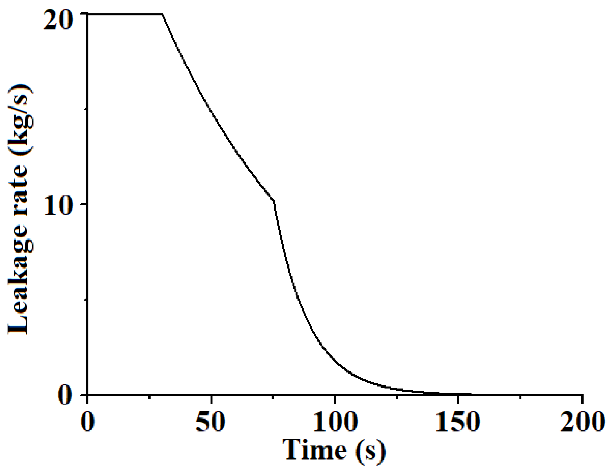
4. Model Application

The validated numerical model is utilized to investigate a gas release scenario on a real offshore platform. The numerical model contributes to acquiring knowledge of the spatial distribution of the released gas, which is essential to derive some practical suggestions.
In this section, a fine geometric model of the target offshore platform is built based on the construction data (Figure 14). Generally, the ESD system and the blowdown system will start sequentially when there is an accidental gas release on offshore platforms. The leakage rate remains unchanged before the ESD starts. Then, the leakage rate decreases exponentially due to depressurization. The starting time of the ESD system and the blowdown system is 30 s and 80 s, respectively, after the gas release [21]. The transient leakage rate profile is calculated accordingly [16], as shown in Figure 15.
The gas consists of 27% methane, 33% ethane, 16% propane, and 24% pentane. The wind blowing towards the accommodation module is selected. The average wind speed at the height of 10 m above the sea is 3 m/s. The ambient temperature is 20 °C.
Figure 16 depicts the variation in FLAM in this scenario. As can be seen, FLAM presents a trend of first increasing and then decreasing. This phenomenon is attributed to the variation in the leakage rate and the dilution in the ventilation. The dilution performance of the ventilation is inadequate for the initial leakage rate, so the FLAM shows an increasing trend before the ESD starts. The leakage rate decreases continuously after the ESD starts. Ventilation plays an increasingly important role by increasing the lean part of the released gas. As a result, the FLAM decreases after a short increase.
Figure 17 illustrates the three-dimensional (3D) spatial distribution of the released gas at different times in the above-mentioned scenario. It can be seen that the distribution range of released gas also first rises and then decreases. It is re-emphasized that the variation in the leakage rate has a great impact on the dispersion behavior and accumulation characteristics of the released gas. The variation in the leakage rate should be considered to acquire a more accurate picture of the accident scenario.
Different from the experimental conditions, ventilation is considered in this scenario. The released gas generally spreads towards the accommodation module under the specified wind direction. It is not hard to imagine that the released gas may enter the accommodation module through the ventilation systems and cause more serious accident consequences. For this reason, forced ventilation blowing away from the accommodation module is recommended, especially in the development of sour oil and gas reservoirs.

5. Summary and Conclusions

An experimental system concerning gas release and dispersion on an offshore platform is established. A series of experiments are carried out. A CFD-based numerical model for gas release and dispersion on the offshore platform is established. The effectiveness of the numerical model is validated by reproducing the experimental scenarios.
It is found that the gas profile is sensitive to the variation in the leakage rate. An obvious lag is observed for the experimental data of concentration. The reason for this is that it takes time for the gas to pass through the rubber tubing, during which the gas will be diluted. In addition, both gas sampling and gas concentration analysis are time-consuming. A series of SPMs are introduced to provide a measure of bias and of spread in the numerical model prediction. And a reasonable agreement with the numerical model is observed for each prediction. The reasons for the differences between the experimental results and the numerical simulation results are also analyzed, such as the difference in the geometry and sampling dimension of the gas detector, the difference in the boundary conditions, and the inherent error of the experimental instrument and the numerical calculation.
Applying the validated numerical model, a typical gas release scenario is investigated, in which a fully transient leakage rate is adopted considering the response of the ESD system and the blowdown system. Significantly, the spatial distribution of the released gas is obtained by the numerical model, from which some practical suggestions are proposed. The current work aims to explore the gas release and dispersion on offshore platforms under different scenarios, especially scenarios with a constant leakage rate or a time-varying leakage rate. A combination of experimental and numerical approaches is adopted in this work, which helps to enhance the awareness of the dispersion characteristics of the released gas. Generally, this work is of great value in many scientific and engineering problems since scenarios with time-varying leakage rates are very common. For example, it is reported that the flowrate during the BP Deepwater Horizon accident is time-varying under the intervention of well control measures. The fire and explosion accidents caused by gas release with a time-varying leakage rate can also be studied on the basis of this study. Equally importantly, this study contributes to providing practical support for risk assessment and contingency planning for gas release accidents.

Author Contributions

Conceptualization, D.Y.; methodology, D.Y.; software, H.D.; validation, H.D.; formal analysis, F.X.; investigation, Y.L.; resources, G.C.; data curation, Y.L.; writing—original draft preparation, F.X.; writing—review and editing, D.Y.; supervision, J.Z.; project administration, J.Z.; funding acquisition, G.C. All authors have read and agreed to the published version of the manuscript.

Funding

This research was funded by the Natural Science Foundation of Shandong Province, China grant number ZR2022QE084, the post-doctoral innovation project of Shandong Province, China grant number SDCX-ZG-202203100, the Project of Ministry of Industry and Information Technology of China grant number CJ09N20, and the Fundamental Research Funds for the Central Universities, China grant number 05Y21030004.

Data Availability Statement

The data presented in this study are available on request from the corresponding author. The data are not publicly available due to privacy.

Conflicts of Interest

Authors Fengpu Xiao, Yanan Li, Jun Zhang, Hai Dong were employed by Engineering Technology Research Institute of Xinjiang Oilfield Company. The remaining authors declare that the research was conducted in the absence of any commercial or financial relationships that could be construed as a potential conflict of interest.

References

  1. Anjana, N.; Amarnath, A.; Nair, M. Toxic hazards of ammonia release and population vulnerability assessment using geographical information system. J. Environ. Manag. 2018, 10, 201–209. [Google Scholar]
  2. Bagheri, M.; Alamdari, A.; Davoudi, M. Quantitative risk assessment of sour gas transmission pipelines using CFD. J. Nat. Gas Sci. Eng. 2016, 31, 108–118. [Google Scholar]
  3. Huang, Y.; Ma, G. A grid-based risk screening method for fire and explosion events of hydrogen refueling stations. Int. J. Hydrog. Energy 2018, 43, 442–454. [Google Scholar]
  4. Dadashzadeh, M.; Khan, F.; Hawboldt, K.; Amyotte, P. An integrated approach for fire and explosion consequence modelling. Fire Saf. J. 2013, 61, 324–337. [Google Scholar]
  5. Dadashzadeh, M.; Abbassi, R.; Khan, F.; Hawboldt, K. Explosion modeling and analysis of BP Deepwater Horizon accident. Saf. Sci. 2013, 57, 150–160. [Google Scholar]
  6. Dadashzadeh, M.; Khan, F.; Abbassi, R.; Hawboldt, K. Combustion products toxicity risk assessment in an offshore installation. Process Saf. Environ. Prot. 2014, 92, 616–624. [Google Scholar]
  7. Gupta, S.; Chan, S. A CFD based explosion risk analysis methodology using time varying release rates in dispersion simulations. J. Loss Prev. Process Ind. 2016, 39, 59–67. [Google Scholar]
  8. Lucas, M.; Skjold, T.; Hiskem, H. Computational fluid dynamics simulations of hydrogen releases and vented deflagrations in large enclosures. J. Loss Prev. Process Ind. 2020, 63, 103999. [Google Scholar]
  9. Baalisampang, T.; Abbassi, R.; Garaniya, V.; Khan, F. Accidental release of liquefied natural gas in a processing facility: Effect of equipment congestion level on dispersion behaviour of the flammable vapour. J. Loss Prev. Process Ind. 2019, 61, 237–248. [Google Scholar]
  10. Mcquaid, J. Heavy Gas Dispersion Trials at Thorney Island; Elsevier: Amsterdam, The Netherlands, 1985; pp. 341–356. [Google Scholar]
  11. Hanna, S.; Chang, J. Use of the Kit Fox field data to analyze dense gas dispersion modeling issues. Atmos. Environ. 2001, 35, 2231–2242. [Google Scholar]
  12. Middha, P.; Hansen, O.; Storvik, I. Validation of CFD-model for hydrogen dispersion. J. Loss Prev. Process Ind. 2009, 22, 1034–1038. [Google Scholar]
  13. Middha, P.; Hansen, O.; Grune, J.; Kotchourko, A. CFD calculations of gas leak dispersion and subsequent gas explosions: Validation against ignited impinging hydrogen jet experiments. J. Hazard. Mater. 2010, 179, 84–94. [Google Scholar]
  14. Savvides, C.; Tam, V.; Kinnear, D. Dispersion of fuel in offshore modules: Comparison of predictions using FLACS and full-scale experiments. In Major Hazards Offshore; ERA Technology Ltd.: London, UK, 2001. [Google Scholar]
  15. Hansen, O.; Gavelli, F.; Ichard, M.; Davis, S. Validation of FLACS against experimental data sets from the model evaluation database for LNG vapor dispersion. J. Loss Prev. Process Ind. 2010, 23, 857–877. [Google Scholar]
  16. Spouge, J. A Guide to Quantitative Risk Assessment for Offshore Installations; CMPT: Aberdeen, SD, USA, 1999. [Google Scholar]
  17. Pan, X.; Jiang, J. Progress of accidental release source and mechanism models. J. Nnajing Univ. Technol. 2002, 24, 105–110. [Google Scholar]
  18. Yang, D.; Chen, G.; Fu, J.; Zhu, Y.; Dai, Z.; Wu, L. The mitigation performance of ventilation on the accident consequences of H2S-containing natural gas release. Process Saf. Environ. Prot. 2021, 148, 1327–1336. [Google Scholar]
  19. Yang, D.; Chen, G.; Shi, J.; Zhu, Y.; Dai, Z. A novel approach for hazardous area identification of toxic gas leakage accidents on offshore facilities. Ocean. Eng. 2020, 217, 107926. [Google Scholar]
  20. GexCon. FLACS v10.4 User’s Manual; GexCon: Bergen, Norway, 2015. [Google Scholar]
  21. API. Manufacturing, Distribution and Marketing Department. In Guide for Pressure-Relieving and Depressuring Systems; American petroleum Institute: Washington, WA, USA, 1997. [Google Scholar]
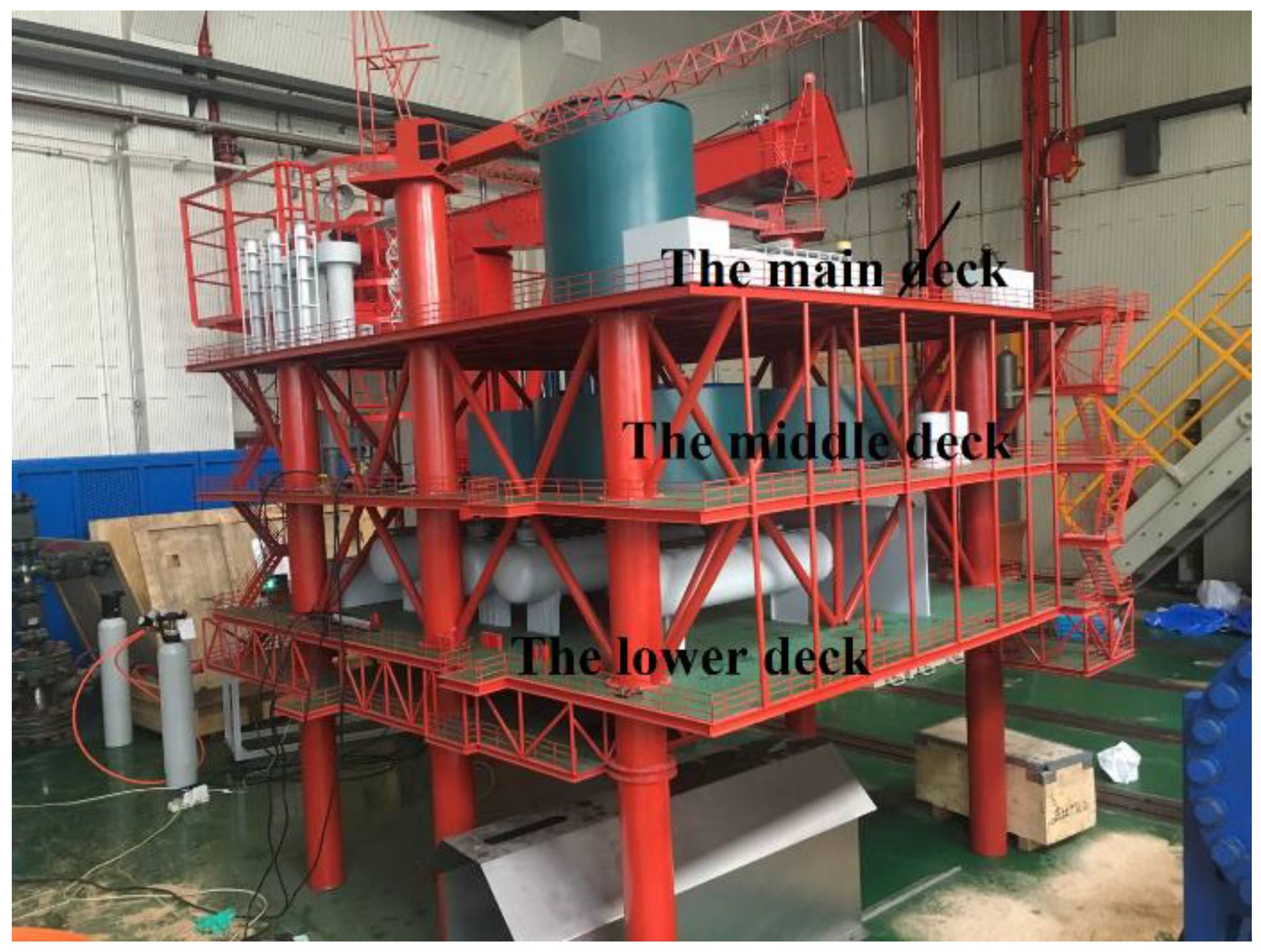
Figure 1. Diagram of the offshore platform gas release and dispersion experimental system.
Processes 11 03437 g001
Figure 2. The experimental offshore platform.
Processes 11 03437 g002
Figure 3. Some devices of the gas leakage module. (a) The gas cylinder with pressure reducing valve. (b) The leakage rate regulator, pressure gauge, and temperature gauge.
Processes 11 03437 g003
Figure 4. A fixed infrared gas detector with natural spread sampling mode.
Processes 11 03437 g004
Figure 5. The layout of the gas detectors.
Processes 11 03437 g005
Figure 6. The variation in gas concentration of monitor #1 against different constant leakage rates.
Processes 11 03437 g006
Figure 7. The variation in gas concentration of different monitors when the leakage rate is 8.1 L/min.
Processes 11 03437 g007
Figure 8. Leakage rate profile for the experiment with a time-varying leakage rate.
Processes 11 03437 g008
Figure 9. The variation in gas concentration of monitor #2 against the time-varying leakage rate.
Processes 11 03437 g009
Figure 10. 3D geometric model of the experimental offshore platform.
Processes 11 03437 g010
Figure 11. The variations in FLAM with different grid sizes.
Processes 11 03437 g011
Figure 12. Comparison between the experimental results and the simulation results against constant leakage rates.
Processes 11 03437 g012
Figure 13. Comparison between the experimental results and the simulation results against the time-varying leakage rate.
Processes 11 03437 g013
Figure 14. Geometric model of the target offshore platform.
Processes 11 03437 g014
Figure 15. Transient leakage rate profile.
Processes 11 03437 g015
Figure 16. FLAM time-varying curve.
Processes 11 03437 g016
Figure 17. Dispersion results of the released gas.
Processes 11 03437 g017
Table 1. Basic dimensions of the experimental offshore platform.
Length (cm)Width (cm)Height (cm)
The whole experimental offshore platform255210308
The main deck255210/
The middle deck255210046
The lower deck255210046
Table 2. Physical and chemical properties of propane gas.
ItemValue or Value RangeItemValue or Value Range
Molecular weight44.10Critical pressure (MPa)4.25
Relative density 1.56Minimus ignition energy (mJ)0.26
Viscosity (kg/m·s)1.01 × 10−5Flashpoint (°C)−104
Saturated vapor pressure (kPa)53.32 (−55.6 °C) Autoignition temperature (°C)450
Critical Temperature (°C)96.8Explosion limit (%)2.1~9.5
Table 3. Time consumed and max. FLAM under different grid sizes.
Grid Size (m)0.150.120.100.075
Computation time (s)6259.298217.889872.2118,834.57
Max. FLAM (m3)0.2890.2480.2370.234
Table 4. Acceptance criteria for different SPM.
SPMMRBMRSEFAC2MGVG
Acceptance criteria−0.4 < MRB < 0.4MRSE < 2.30.5 ≤ FAC20.67 < MG < 1.5VG < 3.3
Table 5. The SPMs of numerical simulation results against constant leakage rates.
SPM4.4 L/min6.2 L/min8.1 L/min
−0.4 < MRB < 0.40.0129−0.0897−0.0877
MRSE < 2.30.00250.00810.0077
0.5 ≤ FAC2 ≤ 20.98851.09401.0920
0.67 < MG < 1.51.0140.91450.9160
VG < 3.31.00261.00821.0078
Table 6. The SPMs of numerical simulation results against the time-varying leakage rate.
SPMMax. ConcentrationMin. Concentration
−0.4 < MRB < 0.4−0.07970.1724
MRSE < 2.30.006350.02972
0.5 ≤ FAC21.0830.841
0.67 < MG < 1.50.9231.189
VG < 3.31.00641.0303
Disclaimer/Publisher’s Note: The statements, opinions and data contained in all publications are solely those of the individual author(s) and contributor(s) and not of MDPI and/or the editor(s). MDPI and/or the editor(s) disclaim responsibility for any injury to people or property resulting from any ideas, methods, instructions or products referred to in the content.

