
Design and Optimization of Precision Fertilization Control System Based on Hybrid Optimized Fractional-Order PID Algorithm

Abstract
:1. Introduction
2. System Design and Model Establishment
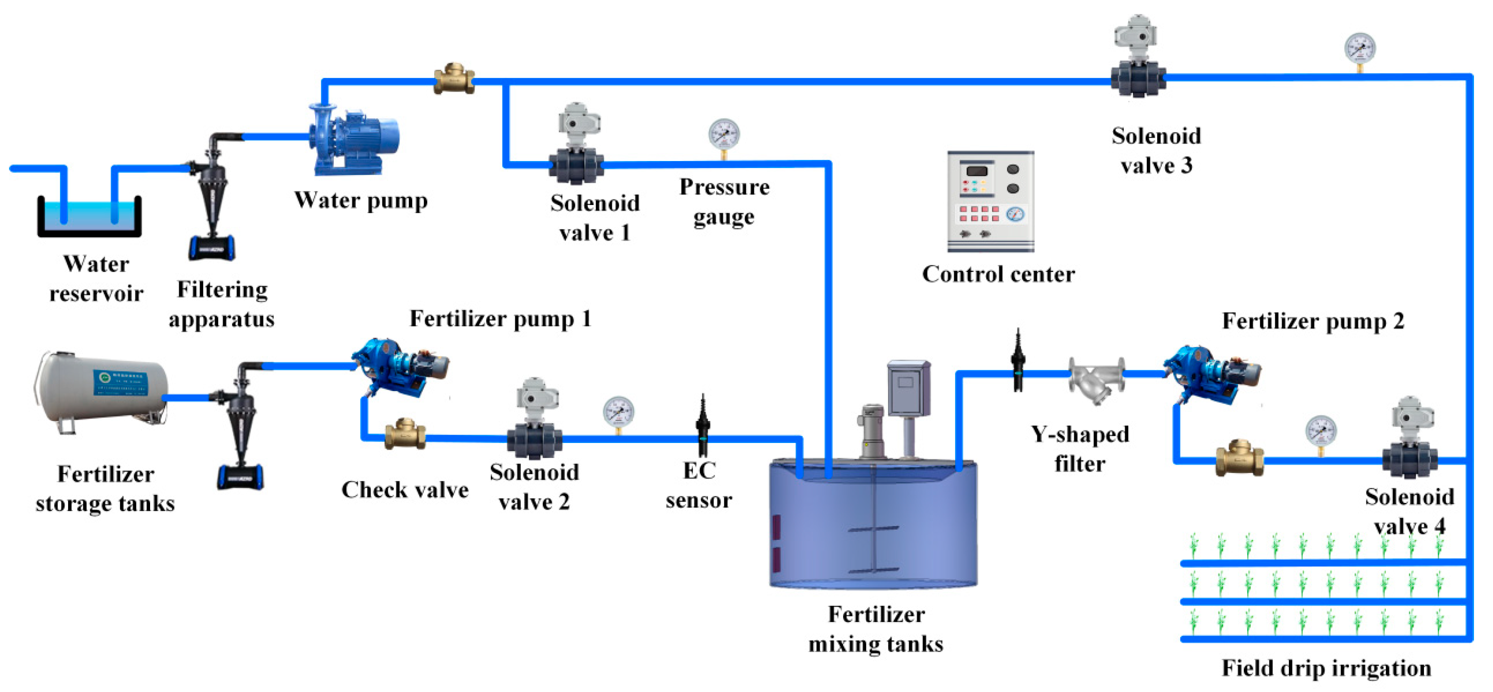
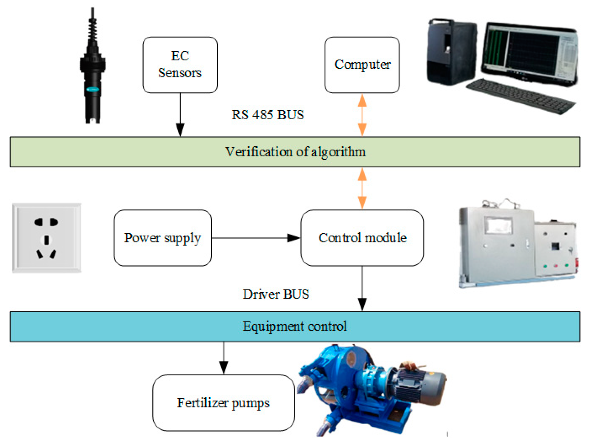
2.1. Construction of a Precision Fertilizer System
2.2. Establishment of Mathematical Model
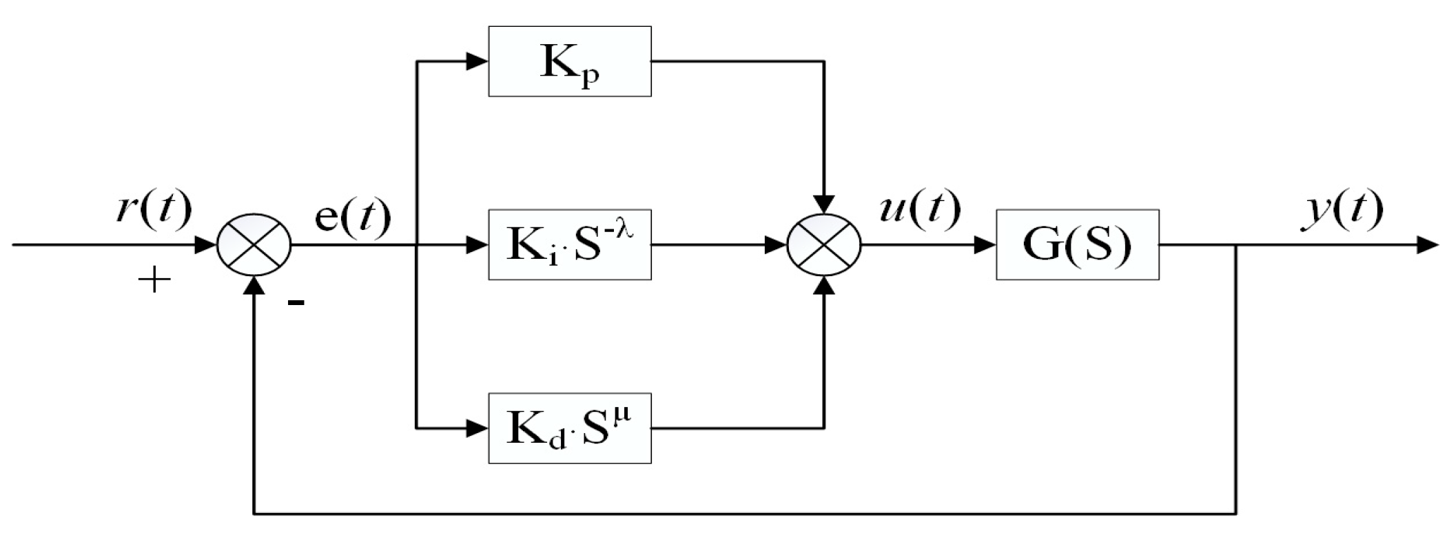
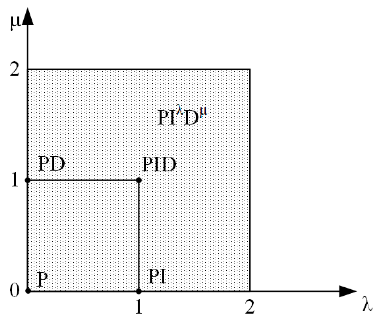
2.3. Fractional-Order PID Controller Design
3. Control Strategy Optimization
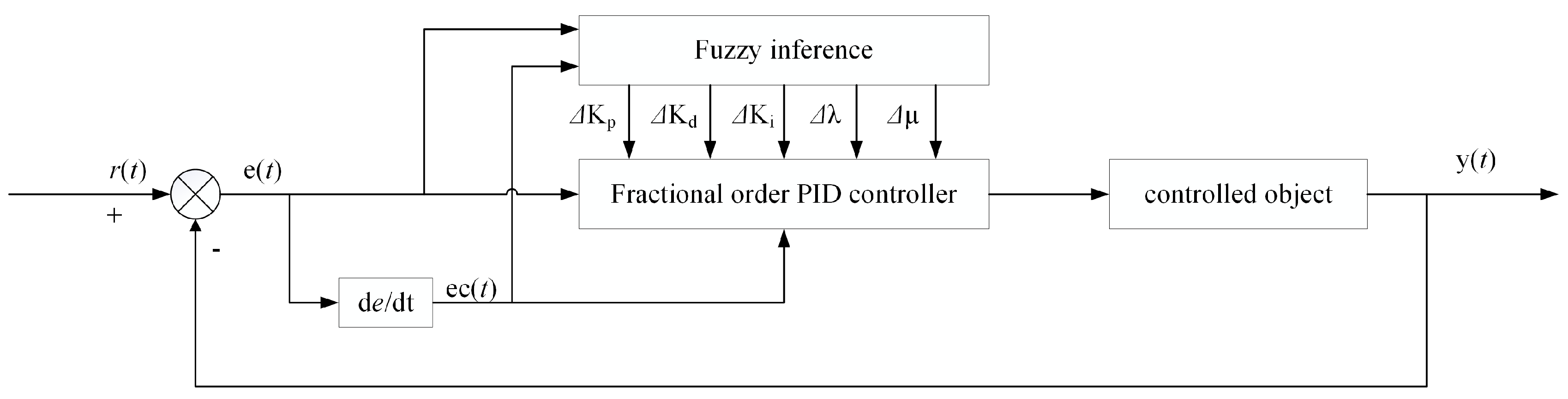
3.1. Controller Parameter Tuning Based on Fuzzy Algorithm
- When the absolute value of error is significantly large, it is advisable to moderately increase and while decreasing . Increasing can enhance the system response rate, reducing can mitigate the impact of disturbance signals, and increasing can minimize system errors.
- When the absolute value of error is moderate, select appropriate values for , , , , and to maintain system stability.
- When the absolute value of error is relatively small, it is advisable to decrease appropriately to reduce the system overshoot. Adjust the values of and based on the error change rate to enhance system stability.
- When the absolute value of the rate of change of the error is significantly large, it is advisable to decrease and while increasing , , and to enhance system damping, reduce system oscillations, and mitigate the impact of the time-variability introduced by delay.
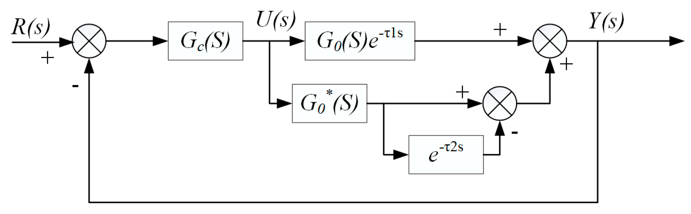
3.2. Structure Optimization Based on Smith Predictor
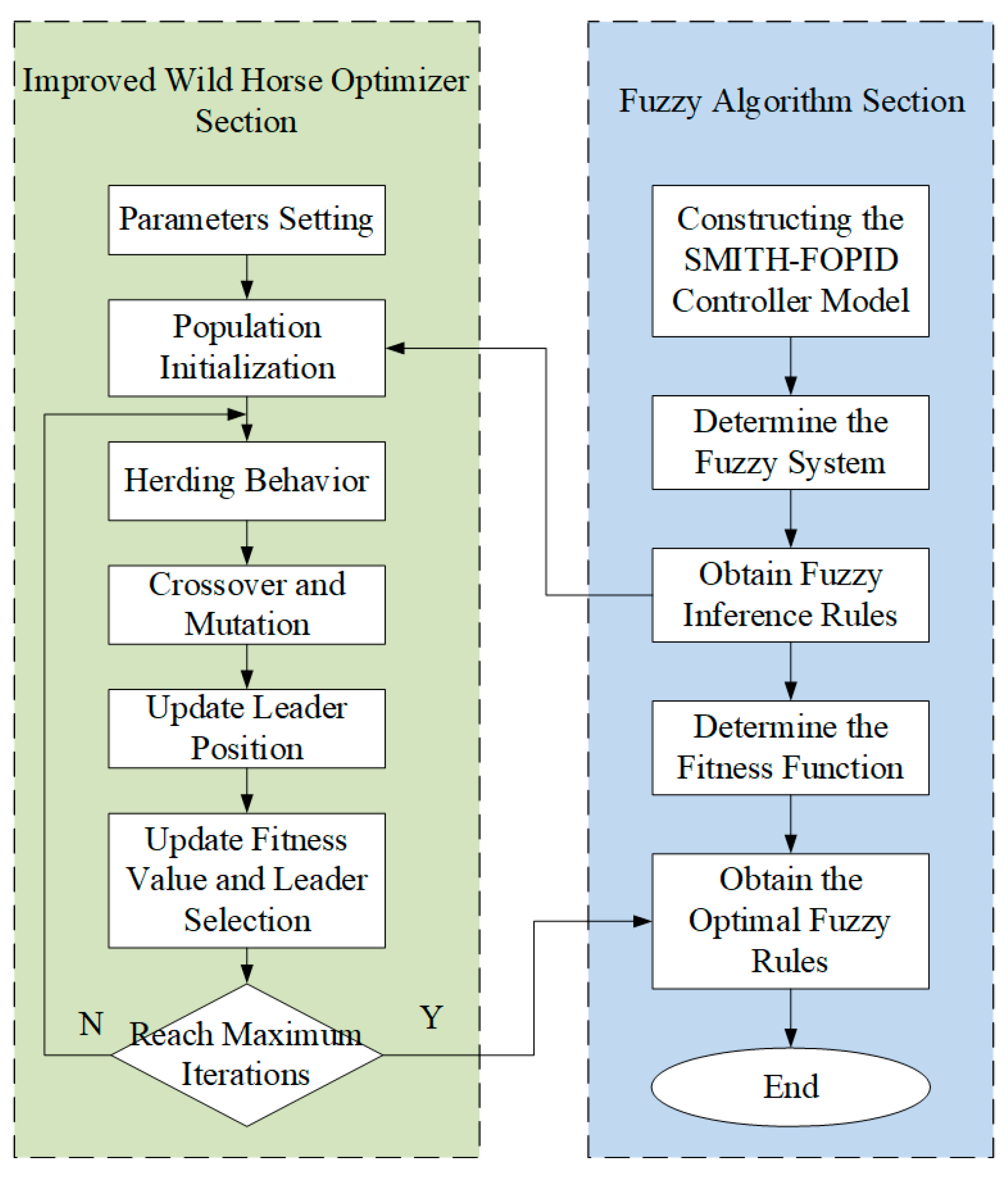
3.3. Parameter Optimization Based on Wild Horse Optimizer
- Population Initialization: For the 49 control rules used in the fuzzy inference process, each horse in the population is represented by a digitized encoding vector for fuzzy linguistic values, where 1, 2, 3, 4, 5, 6, and 7 correspond to NB, NM, NS, ZO, PS, PM, and PB, respectively. The vector length is 49 × 5, and vectors are randomly initialized. The population size was set to , the percentage of stallions as , and the number of groups . These groups were then evenly distributed among the remaining horses in the population.
- Fitness Function: Fitness function reflects superiority or inferiority of individuals, providing a standard and driving force for selection. For the model in this paper, fitness function iswhere represents the PID algorithm’s steady-state time to reach the setpoint, represents the system’s real-time final output, represents objective function setpoint, represents the steady-state time to reach the setpoint and balance after using the optimizing algorithm, and represents the system’s maximum final output value.
- Foraging behavior: The rest of the horses in the herd look around the leader’s position, with the leader’s position as the center of the circle [30]. The expression is given bywhere represents the updated position; is a random number in the range of [−2, 2], primarily used to control the angle between individuals and the leader; is the horse’s position; is the horse’s original position; and is the adaptive mechanism, calculated as follows:where is a vector consisting of 0 s and 1 s, and and are random vectors with values in the interval [0, 1] following a standard distribution. indicates that if an element in is less than , the value at the corresponding position in vector is 1; otherwise, it is 0. Random vector returns the indices where condition (P==0) is satisfied to IDX. is a random number between 0 and 1, represents the dot product operator, represents the binary negation, and is an adaptation factor that decreases linearly from 1 to 0 in the following way:where is the current iteration number, and is the maximum number of iterations.
- Mating Behavior: When the young foal matures, it will leave the herd for mating behavior. Its position-updating method is as follows:where represents the foal ’s position in herd , and , follow the same logic; is the mating method.
- 5.
- Leadership behavior: Each group leader leads the group to a suitable area. Each group moves toward the suitable area. Then, the leaders compete for this suitable area to be used by the ruling group, with no other groups allowed to use the territory until the ruling group leaves. This process is reflected in Equation (18).where represents the group leader’s next position, is an adaptive mechanism, is the current position of the leader, is the position of the suitable area, and is a random number in the range [0, 1].The formula for the leadership selection process is as follows:where represents the individual ’s fitness, and follows the same logic.
- 6.
- Terminating Condition: In this study, the number of iterations is set to 100 generations while using the maximum number of iterations as the final condition.
4. Results
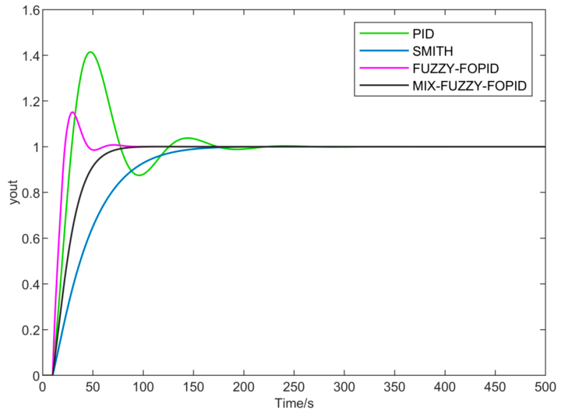
4.1. MATLAB Simulation
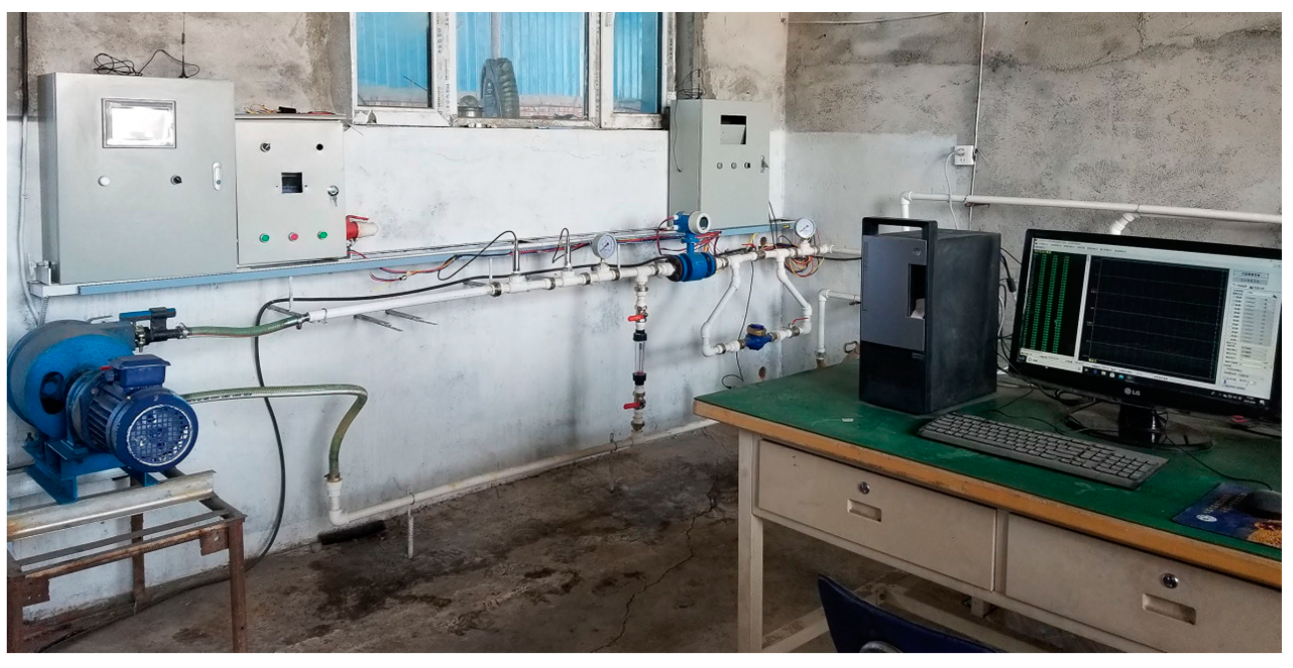
4.2. Experimental Test of EC Adjustment in Precision Fertilization Control System
5. Discussion
6. Conclusions
Author Contributions
Funding
Data Availability Statement
Conflicts of Interest
References
- Shi, Y.; Zhu, Y.; Wang, X.; Sun, X.; Ding, Y.; Cao, W.; Hu, Z. Progress and development on biological information of crop phenotype research applied to real-time variable-rate fertilization. Plant Methods 2020, 16, 11. [Google Scholar] [CrossRef]
- Wang, Y.; Yuan, Y.; Yuan, F.; Ata-UI-Karim, S.T.; Liu, X.; Tian, Y.; Zhu, Y.; Cao, W.; Cao, Q. Evaluation of Variable Application Rate of Fertilizers Based on Site-Specific Management Zones for Winter Wheat in Small-Scale Farming. Agronomy 2023, 13, 2812. [Google Scholar] [CrossRef]
- Raza, A.; Shahid, M.A.; Safdar, M.; Tariq, M.A.R.; Zaman, M.; Hassan, M.U. Exploring the Impact of Digital Farming on Agricultural Engineering Practices. Biol. Life Sci. Forum 2023, 27, 10. [Google Scholar]
- Zhu, F.; Zhang, L.; Hu, X.; Zhao, J.; Meng, Z.; Zheng, Y. Research and Design of Hybrid Optimized Backpropagation (BP) Neural Network PID Algorithm for Integrated Water and Fertilizer Precision Fertilization Control System for Field Crops. Agronomy 2023, 13, 1423. [Google Scholar] [CrossRef]
- Wang, P.; Chen, Y.; Xu, B.; Wu, A.; Fu, J.; Chen, M.; Ma, B. Intelligent Algorithm Optimization of Liquid Manure Spreading Control. Agriculture 2023, 13, 278. [Google Scholar] [CrossRef]
- Bai, J.; Tian, M.; Li, J. Control System of Liquid Fertilizer Variable-Rate Fertilization Based on Beetle Antennae Search Algorithm. Processes 2022, 10, 357. [Google Scholar] [CrossRef]
- Song, L.; Wen, L.; Chen, Y.; Lan, Y.; Zhang, J.; Zhu, J. Variable-Rate Fertilizer Based on a Fuzzy PID Control Algorithm in Coastal Agricultural Area. J. Coast. Res. 2020, 103, 490–495. [Google Scholar] [CrossRef]
- Zhang, J.; Hou, S.; Wang, R.; Ji, W.; Zheng, P.; Wei, S. Design of variable-rate liquid fertilization control system and its stability analysis. Int. J. Agric. Biol. Eng. 2018, 11, 109–114. [Google Scholar] [CrossRef]
- Fu, C.; Ma, X.; Zhang, L. Fuzzy-PID Strategy Based on PSO Optimization for pH Control in Water and Fertilizer Integration. IEEE Access 2022, 10, 4471–4482. [Google Scholar] [CrossRef]
- Wan, C.; Yang, J.; Zhou, L.; Wang, S.; Peng, J.; Tan, Y. Fertilization Control System Research in Orchard Based on the PSO-BP-PID Control Algorithm. Machines 2022, 10, 982. [Google Scholar] [CrossRef]
- Zhou, W.; An, T.; Wang, J.; Fu, Q.; Wen, N.; Sun, X.; Wang, Q.; Liu, Z. Design and Experiment of a Targeted Variable Fertilization Control System for Deep Application of Liquid Fertilizer. Agronomy 2023, 13, 1687. [Google Scholar] [CrossRef]
- Meng, Z.; Zhang, L.; Li, H.; Zhou, R.; Bu, H.; Shan, Y.; Ma, X.; Ma, R. Design and Application of Liquid Fertilizer pH Regulation Controller Based on BP-PID-Smith Predictive Compensation Algorithm. Appl. Sci. 2022, 12, 6162. [Google Scholar] [CrossRef]
- Liu, J.; Yang, C.; Chen, S.; Wang, Y.; Zhang, X.; Kang, W.; Li, J.; Wang, Y.; Hu, Q.; Yuan, X. Hydrochemical Appraisal and Driving Forces of Groundwater Quality and Potential Health Risks of Nitrate in Typical Agricultural Area of Southwestern China. Water 2023, 15, 4095. [Google Scholar] [CrossRef]
- Xu, J.; Wan, W.; Zhu, X.; Zhao, Y.; Chai, Y.; Guan, S.; Diao, M. Effect of Regulated Deficit Irrigation on the Growth, Yield, and Irrigation Water Productivity of Processing Tomatoes under Drip Irrigation and Mulching. Agronomy 2023, 13, 2862. [Google Scholar] [CrossRef]
- Dong, J.; Xue, Z.; Shen, X.; Yi, R.; Chen, J.; Li, Q.; Hou, X.; Miao, H. Effects of Different Water and Nitrogen Supply Modes on Peanut Growth and Water and Nitrogen Use Efficiency under Mulched Drip Irrigation in Xinjiang. Plants 2023, 12, 3368. [Google Scholar] [CrossRef] [PubMed]
- Zhu, J.; Chen, Y.; Li, Z.; Duan, W.; Fang, G.; Wang, C.; He, G.; Wei, W. Using Film-Mulched Drip Irrigation to Improve the Irrigation Water Productivity of Cotton in the Tarim River Basin, Central Asia. Remote Sens. 2023, 15, 4615. [Google Scholar] [CrossRef]
- Wang, W.; Zhang, L.; Ma, X.; Hu, Z.; Yan, Y. Experimental and Numerical Simulation Study of Pressure Pulsations during Hose Pump Operation. Processes 2021, 9, 1231. [Google Scholar] [CrossRef]
- Laldingliana, J.; Biswas, P. Artificial intelligence based fractional order PID control strategy for active magnetic bearing. J. Electr. Eng. Technol. 2022, 17, 3389–3398. [Google Scholar] [CrossRef]
- Guo, B.; Zhuang, Z.; Pan, J.; Chu, s. Optimal design and simulation for PID controller using fractional-order fish migration optimization algorithm. IEEE Access 2021, 9, 8808–8819. [Google Scholar] [CrossRef]
- Padron, J.P.; Perez, J.P.; Diaz, J.J.P.; Astengo-Noguez, C. Time-Delay Fractional Variable Order Adaptive Synchronization and Anti-Synchronization between Chen and Lorenz Chaotic Systems Using Fractional Order PID Control. Fractal Fract. 2023, 7, 4. [Google Scholar] [CrossRef]
- Li, Z.; Ding, J.; Wu, M.; Lin, J. Discrete fractional order PID controller design for nonlinear systems. Int. J. Syst. Sci. 2021, 52, 3206–3213. [Google Scholar] [CrossRef]
- Shi, J. A fractional order general type-2 fuzzy PID controller design algorithm. IEEE Access 2020, 8, 52151–52172. [Google Scholar] [CrossRef]
- Jha, A.K.; Dasgupta, S.S. Fractional order PID based optimal control for fractionally damped nonlocal nanobeam via genetic algorithm. Microsyst. Technol. 2019, 25, 4291–4302. [Google Scholar] [CrossRef]
- Gomaa, H.A.; Yin, Y.Y. A novel optimized fractional-order hybrid fuzzy intelligent PID controller for interconnected realistic power systems. Trans. Inst. Meas. Control 2019, 41, 3065–3080. [Google Scholar] [CrossRef]
- Kacimi, M.A.; Guenounou, O.; Brikh, L.; Yahiaoui, F.; Hadid, N. New mixed-coding PSO algorithm for a self-adaptive and automatic learning of Mamdani fuzzy rules. Eng. Appl. Artif. Intell. 2020, 89, 103417. [Google Scholar] [CrossRef]
- Chen, Y.; Long, F.; Kuang, W.; Zhang, T. A method for predicting blast-induced ground vibration based on Mamdani Fuzzy Inference System. J. Intell. Fuzzy Syst. 2023, 44, 7513–7522. [Google Scholar] [CrossRef]
- Baskys, A. Switched-Delay Smith Predictor for the Control of Plants with Response-Delay Asymmetry. Sensors 2023, 23, 258. [Google Scholar] [CrossRef]
- Naruei, I.; Keynia, F. Wild horse optimizer: A new meta-heuristic algorithm for solving engineering optimization problems. Eng. Comput. 2022, 38 (Suppl. S4), 3025–3056. [Google Scholar] [CrossRef]
- Katoch, S.; Chauhan, S.S.; Kumar, V. A review on genetic algorithm: Past, present, and future. Multimed. Tools Appl. 2021, 80, 8091–8126. [Google Scholar] [CrossRef]
- Zeng, C.; Qin, T.; Tan, W.; Lin, C.; Zhu, Z.; Yang, J.; Yuan, S. Coverage Optimization of Heterogeneous Wireless Sensor Network Based on Improved Wild Horse Optimizer. Biomimetics 2023, 8, 70. [Google Scholar] [CrossRef]


| ec | NB | NM | NS | ZO | PS | PM | PB | |
|---|---|---|---|---|---|---|---|---|
| e | ||||||||
| NB | PB/NB/PS | PB/NB/NS | PM/NM/NB | PM/NM/NB | PS/NS/NB | ZO/ZO/NM | ZO/ZO/PS | |
| NM | PB/NB/PS | PB/NB/NS | PM/NM/NB | PS/NS/NB | PS/NS/NB | ZO/ZO/NM | ZO/ZO/PS | |
| NS | PM/NB/ZO | PM/NM/NS | PM/NS/NM | PM/NS/NM | ZO/ZO/NS | NS/PS/NS | NS/PS/ZO | |
| ZO | PM/NM/ZO | PM/NM/NS | PS/NS/NS | ZO/ZO/NS | NS/PS/NS | NM/PM/NS | NM/PM/ZO | |
| PS | PS/NM/ZO | PS/NS/ZO | ZO/ZO/ZO | NS/PS/ZO | NS/PS/ZO | NM/PM/ZO | NM/PB/ZO | |
| PM | PS/ZO/PB | ZO/ZO/NS | NS/PS/PS | NM/PS/PS | NM/PM/PS | NM/PB/PS | NB/PB/PB | |
| PB | ZO/ZO/PB | ZO/ZO/PM | NM/PS/PM | NM/PM/PM | NM/PM/PS | NB/PB/PS | NB/PB/PB | |
| ec | NB | NM | NS | ZO | PS | PM | PB | |
|---|---|---|---|---|---|---|---|---|
| e | ||||||||
| NB | PB/PS | PB/PS | PM/PB | PM/PB | PS/PB | ZO/PB | ZO/PM | |
| NM | PB/PS | PB/PS | PM/PB | PS/PM | PS/PB | ZO/PB | ZO/PS | |
| NS | PB/ZO | PM/PS | PS/PM | PS/PM | ZO/PN | NS/PM | NS/PS | |
| ZO | PM/ZO | PM/PS | PS/PS | ZO/PS | NS/PS | NM/PS | NM/PS | |
| PS | PM/ZO | PS/ZO | ZO/ZO | NS/ZO | NS/ZO | NM/ZO | NB/ZO | |
| PM | ZO/NB | ZO/NS | NS/NS | NS/NS | NM/NS | NB/NS | NB/NS | |
| PB | ZO/NB | ZO/NM | NS/NM | NM/NS | NM/NS | NB/NS | NB/NS | |
| Controller Type | Rise Time (s) | Peak Time (s) | Regulation Time (s) | Maximum Overshoot |
|---|---|---|---|---|
| PID | 29.13 | 48.01 | 254.28 | 41.43% |
| SMITH | 152.85 | 179.98 | 202.76 | 4.88% |
| Fuzzy-FOPID | 22.55 | 30.26 | 128.37 | 15.59% |
| Mix-Fuzzy-FOPID | 86.94 | 94.08 | 114.61 | 1.63% |
| Controller Type | Target EC Values (mS/cm) | Steady-State EC Values (mS/cm) | EC Fluctuation Amplitude (mS/cm) | Steady-State Time (s) | Overshoot (%) |
|---|---|---|---|---|---|
| PID | 1.5 | 1.21~1.82 | 0.61 | 218 | 21.4 |
| 1.8 | 1.57~2.14 | 0.57 | 223 | 21.7 | |
| 2.0 | 1.73~2.26 | 0.53 | 236 | 22.9 | |
| SMITH | 1.5 | 1.39~1.75 | 0.36 | 183 | 15.7 |
| 1.8 | 1.61~1.94 | 0.33 | 189 | 16.0 | |
| 2.0 | 1.85~2.17 | 0.32 | 197 | 16.3 | |
| Fuzzy-FOPID | 1.5 | 1.33~1.92 | 0.59 | 151 | 19.5 |
| 1.8 | 1.57~2.08 | 0.51 | 169 | 20.2 | |
| 2.0 | 1.87~2.31 | 0.44 | 176 | 20.8 | |
| Mix-Fuzzy-FOPID | 1.5 | 1.43~1.58 | 0.15 | 92 | 10.1 |
| 1.8 | 1.76~1.89 | 0.13 | 101 | 10.9 | |
| 2.0 | 1.94~2.03 | 0.09 | 112 | 12.4 |
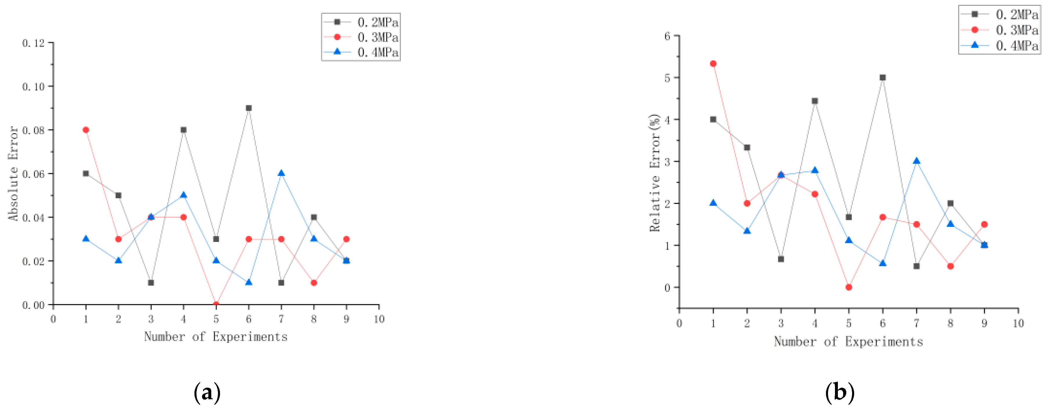
| Target EC Values (mS/cm) | 0.2 MPa | 0.3 MPa | 0.4 MPa | ||||||
|---|---|---|---|---|---|---|---|---|---|
| Measured Mean (mS/cm) | Absolute Error (mS/cm) | Relative Error (%) | Measured Mean (mS/cm) | Absolute Error (mS/cm) | Relative Error (%) | Measured Mean (mS/cm) | Absolute Error (mS/cm) | Relative Error (%) | |
| 1.5 | 1.56 | 0.06 | 4.00 | 1.58 | 0.08 | 5.33 | 1.47 | 0.03 | 2.00 |
| 1.45 | 0.05 | 3.33 | 1.53 | 0.03 | 2.00 | 1.52 | 0.02 | 1.33 | |
| 1.51 | 0.01 | 0.67 | 1.54 | 0.04 | 2.67 | 1.54 | 0.04 | 2.67 | |
| 1.8 | 1.88 | 0.08 | 4.44 | 1.76 | 0.04 | 2.22 | 1.85 | 0.05 | 2.78 |
| 1.83 | 0.03 | 1.67 | 1.80 | 0.00 | 0.00 | 1.78 | 0.02 | 1.11 | |
| 1.89 | 0.09 | 5.00 | 1.83 | 0.03 | 1.67 | 1.81 | 0.01 | 0.56 | |
| 2.0 | 1.99 | 0.01 | 0.50 | 1.97 | 0.03 | 1.50 | 1.94 | 0.06 | 3.00 |
| 1.96 | 0.04 | 2.00 | 2.01 | 0.01 | 0.50 | 2.03 | 0.03 | 1.50 | |
| 2.02 | 0.02 | 1.00 | 2.03 | 0.03 | 1.50 | 1.98 | 0.02 | 1.00 | |
Disclaimer/Publisher’s Note: The statements, opinions and data contained in all publications are solely those of the individual author(s) and contributor(s) and not of MDPI and/or the editor(s). MDPI and/or the editor(s) disclaim responsibility for any injury to people or property resulting from any ideas, methods, instructions or products referred to in the content. |
© 2023 by the authors. Licensee MDPI, Basel, Switzerland. This article is an open access article distributed under the terms and conditions of the Creative Commons Attribution (CC BY) license (https://creativecommons.org/licenses/by/4.0/).
Share and Cite
Wang, H.; Zhang, L.; Hu, X.; Wang, H. Design and Optimization of Precision Fertilization Control System Based on Hybrid Optimized Fractional-Order PID Algorithm. Processes 2023, 11, 3374. https://doi.org/10.3390/pr11123374
Wang H, Zhang L, Hu X, Wang H. Design and Optimization of Precision Fertilization Control System Based on Hybrid Optimized Fractional-Order PID Algorithm. Processes. 2023; 11(12):3374. https://doi.org/10.3390/pr11123374
Chicago/Turabian StyleWang, Hao, Lixin Zhang, Xue Hu, and Huan Wang. 2023. "Design and Optimization of Precision Fertilization Control System Based on Hybrid Optimized Fractional-Order PID Algorithm" Processes 11, no. 12: 3374. https://doi.org/10.3390/pr11123374
APA StyleWang, H., Zhang, L., Hu, X., & Wang, H. (2023). Design and Optimization of Precision Fertilization Control System Based on Hybrid Optimized Fractional-Order PID Algorithm. Processes, 11(12), 3374. https://doi.org/10.3390/pr11123374