An Expert System Based on Data Mining for a Trend Diagnosis of Process Parameters

Abstract

In order to diagnose abnormal trends in the process parameters of industrial production, the Expert System based on rolling data Kernel Principal Component Analysis (ES-KPCA) and Support Vector Data Description (ES-SVDD) are proposed in this paper. The expert system is capable of identifying large-scale trend changes and abnormal fluctuations in process parameters using data mining techniques, subsequently triggering timely alarms. The system consists of a rule-based assessment of process parameter stability to evaluate whether the process parameters are stable. Also, when the parameters are unstable, the rolling data-based KPCA and SVDD methods are used to diagnose abnormal trends. ES-KPCA and ES-SVDD methods require adjusting seven threshold parameters during the offline parameter adjustment phase. The system obtains the adjusted parameters and performs a real-time diagnosis of process parameters based on the set diagnosis interval during the online diagnosis phase. The ES-KPCA and ES-SVDD methods emphasize the real-time alarms and the first alarm of process parameter abnormal trends, respectively. Finally, the system validates the experimental data from UniSim simulation and a chemical plant. The results show that the expert system has an outstanding diagnostic performance for abnormal trends in process parameters.

1. Introduction

Equipment and devices in industrial production are often influenced by equipment failures, environmental changes, and human errors, which may lead to abnormal process parameters. Abnormal process parameters can negatively impact production efficiency, product quality, and operational safety [1]. Industrial processes involve many process parameters, such as temperature, pressure, and flow rate, and their ability to remain stable is crucial for product quality, safety, and efficiency [2,3]. Typically, these process parameters are configured with alarm thresholds, but there are noticeable trend abnormalities and fluctuations before reaching alarm thresholds without corresponding alarm notifications. Therefore, the diagnosis and alarm of abnormal trends in process parameters precisely address this limitation, and issuing trend-based alarms before reaching the alarm thresholds serves as an early warning. It plays a crucial role in on-site emergency handling, inspection, and maintenance, providing key advantages regarding timeliness and advance [4,5].

Researchers have recently proposed various methods for diagnosing abnormal process parameters, including clustering-based methods, density-based methods, data-driven methods, and expert system methods [6,7,8,9]. The clustering-based approach involves clustering the data of parameters into multiple clusters, where the cluster with the least data points is considered to be the abnormal cluster. In this method, the k-means algorithm [10,11] is widely used and recognized, but it requires predefining the number of clusters and is sensitive to the initial points, which can make diagnosis difficult and hinder the detection of outliers. The density-based approach identifies outliers based on the density distribution of the data [12,13]. Zheng et al. [14] referenced a study on automatic modulation classification, which employed spectrum interference and data augmentation techniques to expand the training dataset, potentially improving the anomaly trend analysis. However, this method has problems, such as the need for many samples and the difficulty in making assumptions about the data distribution. The data-driven approach is a technique that utilizes the features and patterns of historical or real-time data to detect potential anomalies. Li et al. [15] integrated data-driven methods in the context of multi-agent consensus in supply chain systems, which are essential for fault diagnosis. Zheng et al. [16] introduced a prior regularization method in deep learning (DL-PR) to enhance the accuracy of automatic modulation classification (AMC), thereby improving the performance of deep learning models, especially in complex environments. The expert system approach involves building a knowledge base and reasoning mechanism to simulate the decision-making process of human experts [17]. Nowak et al. [18] analyzed the use of Local Outlier Factor (LOF), Connectivity-Based Outlier Factor (COF), and k-means algorithms for outlier detection in rule-based knowledge bases and achieved promising results.

In this paper, data mining is adopted to diagnose abnormal trends in process parameters, including KPCA, SVDD, and Radial Basis Function Convolutional Neural Network (RBF-CNN). Firstly, KPCA maps the data into a high-dimensional feature space and calculates the principal components using kernel functions, thereby achieving data dimensionality reduction and feature extraction [19]. Secondly, the SVDD method transforms the dataset from the original space to a feature space using nonlinear transformations and then searches for the smallest volume hypersphere within the feature space [20]. Lastly, RBF-CNN conducts feature extraction through convolutional and pooling layers, and the weights of the convolutional kernels and parameters of the pooling layers are optimized through neural network training [21]. Unlike the characteristics of control loops, process parameters possess numerous features, and historical data often fail to include all of them. Therefore, the diagnosis of process parameters relies on comparing the similarity of recent data features to diagnose parameter anomalies. As the variations in process parameters typically occur rapidly, this diagnosis requires a high degree of real-time capability. The KPCA and SVDD methods excel in feature extraction with fast processing and outstanding real-time capabilities, making them suitable for parameter diagnosis. In contrast, the RBF-CNN method has a slower training speed and is unsuitable for parameter diagnosis. Among these three methods, only the KPCA approach alters the data dimensions. KPCA’s fundamental concept involves the nonlinear mapping of the input space into a high-dimensional feature space. In this process, its data are projected along the path of maximum variance, and kernel functions are applied to capture the process’s nonlinear features. Zhu et al. [22] integrated KPCA with deep learning for applications in the field of fault diagnosis. Ned et al. [23] proposed a partial least squares (PLS) method tailored to multistage batch processes, which better reflects the dynamic characteristics of actual processes. However, extracting features and identifying multiple transition points require understanding the process. Fazai et al. [24] proposed a fusion of the generalized likelihood ratio test with the Partial Least Squares (PLS) method to establish a fault detection model for application in chemical process monitoring. Dimoudis et al. [25,26] used an adaptive window with the rolling median method for time-series anomaly detection for real-time diagnosis. Rafferty et al. [27] and Dong et al. [28] introduced sliding window PCA and process monitoring PCA algorithms for real-time fault diagnosis. However, these are unsuitable for nonlinear and single-process parameter scenarios.

The core concept of SVDD is to construct a hypersphere that maximally encloses the positive samples in the training set and achieves the greatest separation between positive and negative samples. Tax and Duin initially proposed the SVDD method based on the support vector foundation [29]. They further refined the SVDD model and demonstrated the feasibility of using kernel functions instead of inner product operations. Additionally, when employing a radial basis kernel function, it can be proven that the SVDD and One-Class Support Vector Machine (OCSVM) methods are equivalent and consistent with the findings in reference [30]. Zhang et al. [31] combined the Kernel-based Incremental Support Vector Data Description (KISVDD) with a sliding window for fault diagnosis, focusing only on positive samples during training. However, their approach might lack flexibility in handling abnormal samples, potentially leading to performance degradation, especially for adjacent anomalies.

It is generally challenging to detect all types of anomalies in process parameters using a single algorithm. Therefore, research on expert systems in chemical safety has gained increasing attention. Expert system rules are a fundamental form of knowledge in expert systems, representing a set of rules established by domain experts to describe the knowledge and experiences in a specific field. These rules are typically structured as ‘IF-THEN’ [32]. Guo et al. [33] designed 22 expert system rules for diagnosing variable refrigerant flow parameters. However, the comprehensive handling of individual expert system knowledge is often difficult and inefficient. As a result, researchers commonly combine rules with other methods. Zhou et al. [34] proposed an integrated framework of machine learning and expert systems to enhance the flexibility and efficiency of building energy management. This approach leverages solar photovoltaic and battery technology to reduce electricity costs and enable adaptability to changing external conditions.

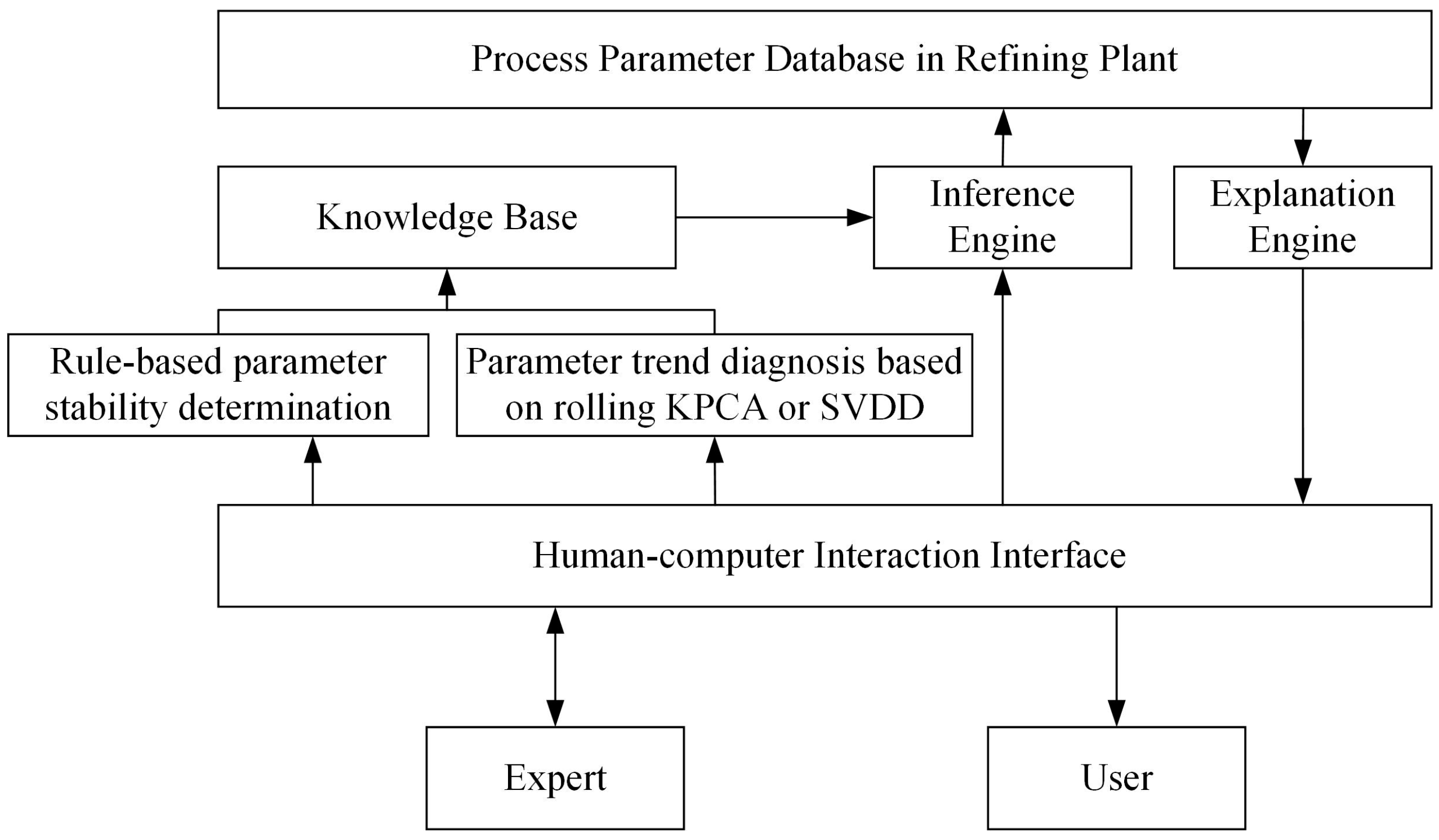
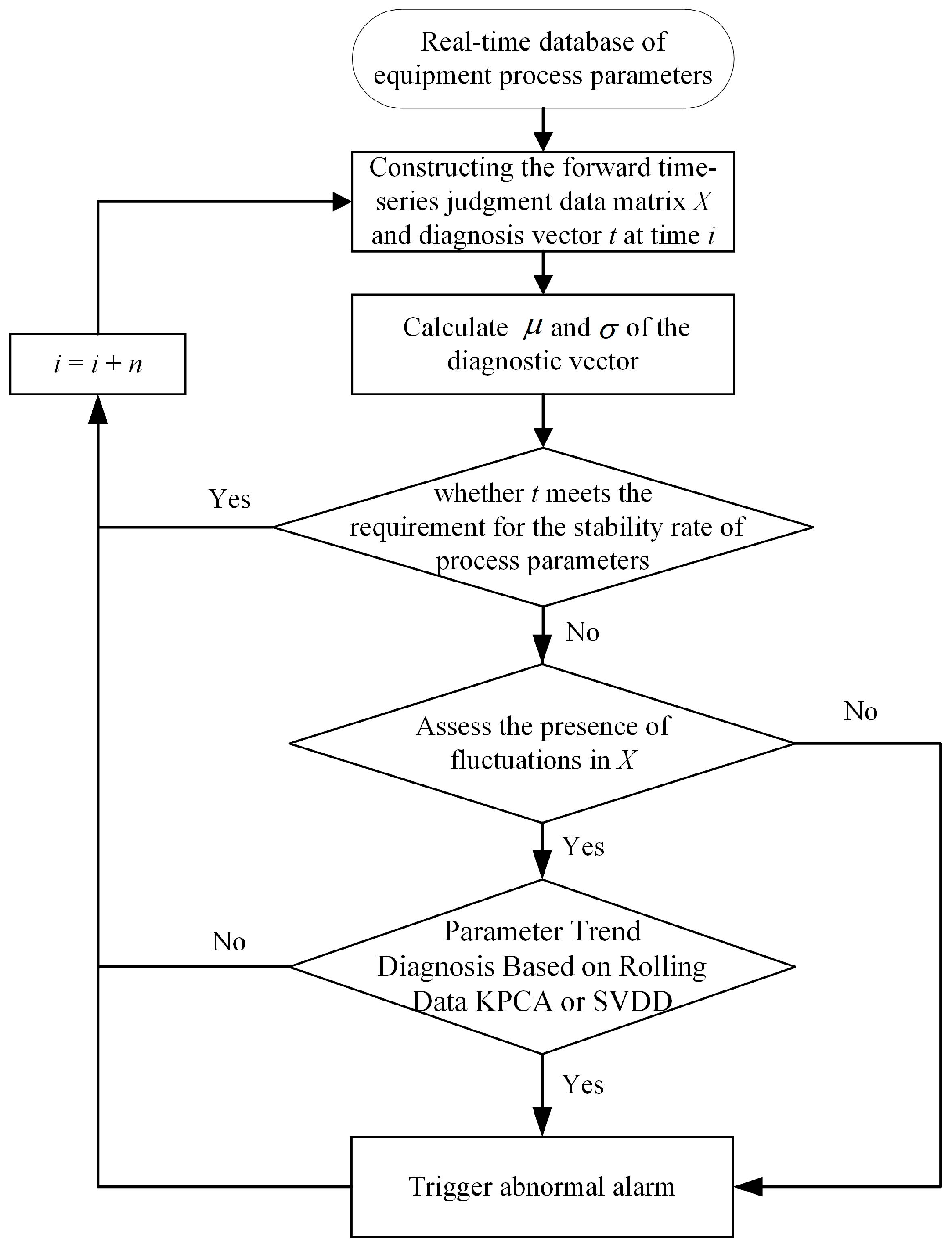
In conclusion, this paper integrates expert rules with data-driven methods to design and apply the ES-KPCA and ES-SVDD methods. The system combines a rule-based assessment of process parameter stability with rolling data KPCA and SVDD diagnosis of process parameter trend anomalies. Its objective is to enhance the accuracy and efficiency of detecting nonlinear single-process parameter anomalies in industrial production. It should be noted that rolling data are essentially equivalent to sliding windows, but the rolling data-based KPCA method is distinct from Sliding Window KPCA [35]. Sliding windows focus on data within a fixed window that moves along the data to capture different periods and are commonly used in statistical and time series analyses. This paper constructs rolling data by building a rolling data matrix and comparing the similarity between diagnosis vectors and forward time-series judgment data matrices, emphasizing real-time analysis. Finally, the system is validated and evaluated using actual data from a domestic refining and chemical plant and UniSim simulation data, demonstrating its effectiveness and practicality in real-world applications.

2. Basic Overview

2.1. Process Parameters in the Process Industry

Process parameters are essential in the process industry, as they significantly impact the product quality and production efficiency in different units and process steps [36]. These parameters include temperature, pressure, flow rate, catalyst feed rate, hydrogen usage, and ratios. Maintaining the critical process parameters within normal ranges is crucial for producing high-quality products and improving production efficiency. Abnormalities in these parameters can result in a reduced production quality, decreased product yield, increased energy consumption, and other issues.

2.2. Abnormal Trend Diagnosis of Process Parameters

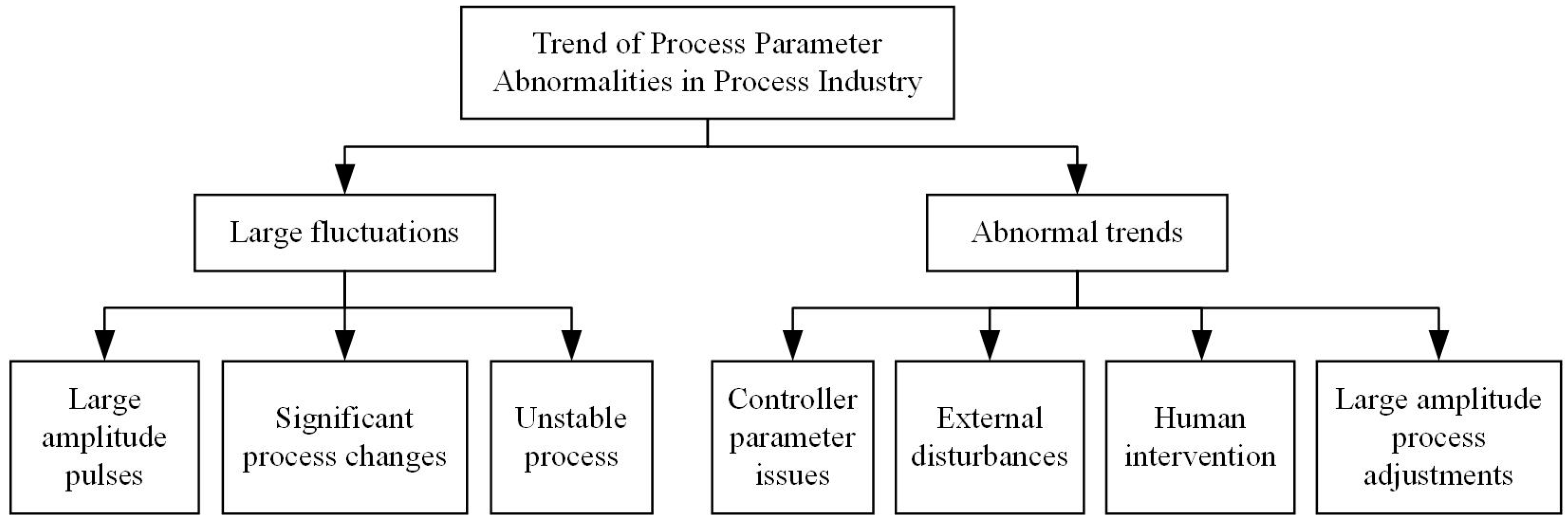
The trend diagnosis of process parameters in refining units is a method for monitoring and analyzing process parameters to determine whether they exhibit stable behavior or abnormal trends. Various causes can lead to abnormal trends in process parameters, such as operational errors by operators, possible damage or wear of equipment components, potential blockages in pumps or valves, and extreme weather conditions, which can adversely affect production units. Figure 1 illustrates the abnormal trends and causes of process parameters in a refining unit. Abnormal trends can be categorized as large fluctuations and abnormal trends.

2.3. Rolling Data Matrix

The data set collected for process parameters in the industry has only two features: timestamps and parameter values. To conduct a trend diagnosis for the process parameters, they are elevated to higher dimensions based on their chronological order in the time series. As shown in Equation (1), using different real-time moments $i$ as the basis, the most recent parameter column vector is constructed as the diagnosis vectors for discrimination. Subsequently, a forward time series judgment data matrix is formed for comparison based on similarity. Each matrix column represents the process parameter values for a specific period, incrementally rolling forward with the increase in $i$.

$$\begin{array}{c}\left[\begin{array}{lllll}{x}_{i-(mn-1)}& x_{i-\left[\right(m-1)n-1]}& x_{i-\left[\right(m-2)n-2]}& \cdots & x_{i-(2n-1)}\\ x_{i-(mn-2)}& x_{i-\left[\right(m-1)n-2]}& x_{i-\left[\right(m-2)n-2]}& \cdots & x_{i-(2n-2)}\\ x_{i-(mn-3)}& x_{i-\left[\right(m-1)n-3]}& x_{i-\left[\right(m-2)n-3]}& \cdots & x_{i-(2n-3)}\\ ⋰& ⋰& ⋰& & ⋰\\ x_{i-mn}& x_{i-(m-1)n}& x_{i-(m-2)n}& \cdots & x_{i-n}\end{array}\right]\left[\begin{array}{l}{x}_{i-(n-1)}\\ x_{i-(n-2)}\\ x_{i-(n-3)}\\ ⋰\\ x_i\end{array}\right]\\ \mathrm{Forward}\mathrm{time-series}\mathrm{judgment}\mathrm{data}\mathrm{matrix}\mathrm{Diagnosis}\mathrm{vector}\end{array}$$

(1)

where $x_i$ is the process parameter data, $n$ is the rolling step, $m$ is the number of samples in the judgment data matrix, and $i$ is the current moment.

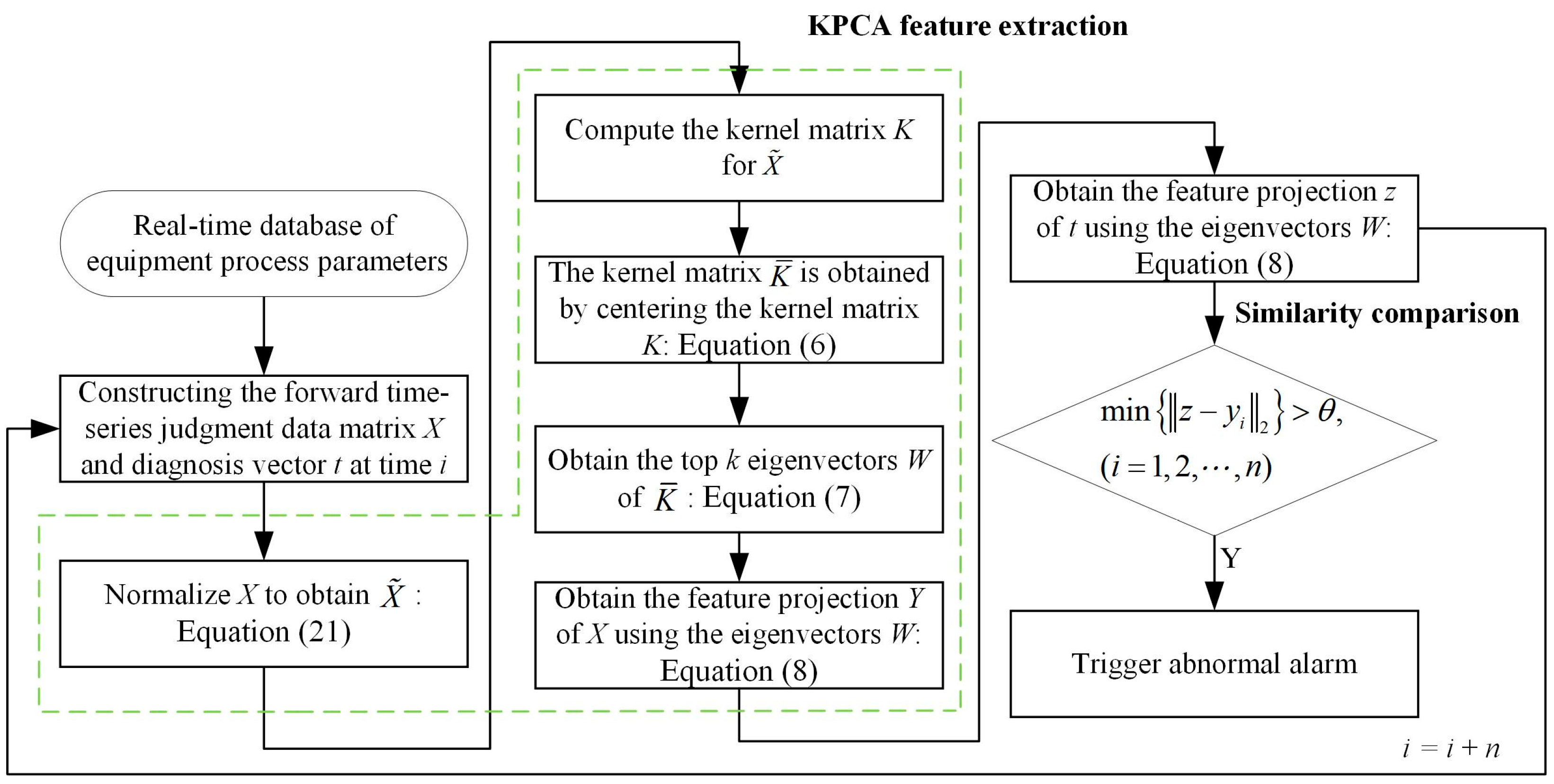
2.4. KPCA

KPCA is a kernel function-based principal component analysis method that maps high-dimensional data into a low-dimensional space to discover the main features and structure of the data. Unlike traditional PCA methods, KPCA uses kernel functions instead of linear transformations and can handle nonlinear data and preserve the nonlinear structure of the original data in a low-dimensional space [19]. To make the maximum data variance information retained in the new low-dimensional space, KPCA uses Singular Value Decomposition (SVD) to compute the linear transformation matrix $W$ [37]. The feature extraction steps are as follows:

Suppose the original data set is $X={[x_1,x_2,\cdots ,x_n]}^{\mathrm{T}}\in {\mathrm{R}}^{n\times m}$ and $x_i=[x_{i1},x_{i2},\cdots ,x_{im}]$. A nonlinear mapping function $\Phi$ is introduced to project the original data set $X$ into the high-dimensional feature space $F$. The covariance matrix $A$ of the high-dimensional feature space is expressed as:

$$A=\frac{1}{n}{\displaystyle \sum _{i=1}^n\Phi (x_i)\Phi {(x_i)}^{\mathrm{T}}}$$

(2)

Let $\lambda$ be the eigenvalues of the covariance matrix $A$, and $V$ be the corresponding eigenvectors. Then, the eigenvalue problem for $A$ is expressed as:

$$\lambda V=AV=\left\{\frac{1}{n}{\displaystyle \sum _{i=1}^n\Phi (x_i){[\Phi (x_i)]}^{\mathrm{T}}}\right\}V=\frac{1}{n}{\displaystyle \sum _{i=1}^n〈\Phi (x_i),V〉\Phi (x_i)}$$

(3)

where the symbol 〈 〉 denotes the inner product, and $V$ in the feature space is expressed as:

$$V={\displaystyle \sum _{i=1}^n{\alpha }_i\Phi (x_i)}$$

(4)

where ${\alpha }_i$ is a constant factor.

The new equation is obtained by taking the inner product of both sides of the equation in Equation (2) and combining it with Equation (3).

$$\lambda {\displaystyle \sum _{i=1}^n{\alpha }_i〈\Phi (x_i),\Phi (x_k)〉}=\frac{1}{n}{\displaystyle \sum _{i=1}^n{\displaystyle \sum _{j=1}^n{\alpha }_i〈\Phi (x_i),\Phi (x_j)〉〈\Phi (x_i),\Phi (x_k)〉}}$$

(5)

The $n\times n$ kernel matrix $K(x_i,x_j)=〈\Phi (x_i),\Phi (x_j)〉$ is introduced to avoid high-dimensional operations, leading to the kernel matrix $K$. The prevalent kernel functions encompass the linear, polynomial, Gaussian, and Sigmoid types, with the selection contingent upon specific needs.

The kernel matrix $K$ is then subjected to centering processing.

$$\overline{K}=K-IK-KI-IKI$$

(6)

where $I$ is an $n\times n$ dimensional identity matrix with coefficients of $1/n$.

With Equation (4), the eigenvalue problem for $\overline{K}$ is expressed as:

$$\lambda \alpha =\frac{1}{n}\overline{K}\alpha$$

(7)

The selection of kernel principal components depends on $\lambda$ Select the eigenvectors corresponding to the first $k(k<n)$ larger eigenvalues to reduce the dimensionality of the data. The matrix composed of k eigenvectors is denoted as $W={[{\alpha }_1,{\alpha }_2,\cdots ,{\alpha }_k]}^{\mathrm{T}}\in R^{k\times n}$, where ${\alpha }_i=[{\alpha }_{i1},{\alpha }_{i2},\cdots ,{\alpha }_{in}]$, $(i=1,2,\cdots ,k)$.

The original data matrix $X$ undergoes a linear transformation through the matrix $W$, resulting in its projection on the feature space:

$$Y=W^{\mathrm{T}}\Phi \left(X\right)$$

(8)

Due to the capability of KPCA to perform nonlinear transformations, it is suitable for various types of data.

2.5. SVDD

The basic idea of SVDD is to construct a hyperborder to form a hypersphere to contain as many positive samples as possible in the training samples and achieve the maximum separation of positive and negative samples [38,39]. The core problem of SVDD is to find the optimal bound to achieve the optimal detection effect.

Suppose there is a set of normal training data $x\in R^{m\times n}$, where $m$ is the number of samples and $n$ is the feature dimension. The data are mapped from the original space to the feature space with the nonlinear transformation function $\Phi :x\to F$, and a hypersphere with the smallest volume is found in the feature space. Refer to Equation (9) for details:

$$\left\{\begin{array}{l}\underset{a,R,\xi }{\min }{R}^2+C{\displaystyle \sum _{i=1}^m{\xi }_i}\\ s.t.{(x_i-a)}^T(x_i-a)\le R^2+{\xi }_i({\xi }_i\ge 0,\forall i=1,2,\dots m)\end{array}\right.$$

(9)

where $R$ is the radius of the hypersphere, $a$ is the center of the hypersphere circle, ${\xi }_i\ge 0$ is the relaxation variable, and $C$ is a constant whose role is to control the minimization of the radius $a$ and the trade-off of the relaxation variable.

Combined with the Lagrange multiplier method, Equation (9) can be transformed into the dual problem of Equation (10) as follows:

$$\left\{\begin{array}{l}\underset{{\tau }_i}{\min }{\displaystyle \sum _{i=1}^m{\displaystyle \sum _{j=1}^m{\tau }_i{\tau }_{j}K(x_i,x_j)-{\displaystyle \sum _{i=1}^m{\tau }_{i}K(x_i,x_i)}}}\\ s.t.0\le {\tau }_i\le C,{\displaystyle \sum _{i=1}^m{\tau }_i=1}\end{array}\right.$$

(10)

where ${\tau }_i$ is the Lagrange coefficient corresponding to $x_i$.

In cases where the hypersphere boundary cannot ensure precise classification, the SVDD can be enhanced using the kernel function approach. This involves mapping the training data to a higher-dimensional space for hypersphere calculations.

Among all the normal training samples, the samples for which the Lagrange coefficients satisfy $0<{\tau }_i<C$ are referred to as support vectors. The set of support vectors belonging to the training dataset is denoted as SV and can be used to compute the center and radius of the hypersphere using Equation (11).

$$\left\{\begin{array}{l}a={\displaystyle \sum _{i=1}^m{\tau }_i\Phi (x_i)}\\ R=\sqrt{K(x_v,x_v)-2{\displaystyle \sum _{i=1}^m{\tau }_{i}K(x_v,x_i)+{\displaystyle \sum _{i=1}^m{\displaystyle \sum _{j=1}^m{\tau }_i{\tau }_{j}K(x_i,x_j)}}}}\end{array}\right.$$

(11)

where $v\in SV$ and $K(x_i,x_j)$ is the Kernel function. The prevalent kernel functions encompass the linear, polynomial, Gaussian, and Sigmoid types, with the selection contingent upon specific needs.

For a test sample $x_t$, calculate its distance to the center of the hypersphere:

$$d=\sqrt{K(x_t,x_t)-2{\displaystyle \sum _{i=1}^m{\tau }_{i}K(x_t,x_i)+{\displaystyle \sum _{i=1}^m{\displaystyle \sum _{j=1}^m{\tau }_i{\tau }_{j}K(x_i,x_j)}}}}$$

(12)

If $d\le bR(b\ge 1)$, it indicates that the test sample is on or inside the surface of the hypersphere and belongs to the normal samples. Conversely, if $d>bR(b\ge 1)$, it belongs to the abnormal samples.

In the actual training process, it is recommended to include a small number of negative class samples in the training set of positive class samples to prevent overfitting. Let us assume that the positive class samples and negative class samples in the training set are labeled as follows:

$$\left\{\begin{array}{l}{y}_i=+1\\ y_j=-1\end{array}\right.$$

(13)

The dual problem is then transformed as:

$$\left\{\begin{array}{l}\underset{{\alpha }_i}{\min }{\displaystyle \sum _{i=1}^m{\displaystyle \sum _{j=1}^m{y}_i{y}_j{\tau }_i{\tau }_{j}K(x_i,x_j)-{\displaystyle \sum _{i=1}^m{y}_i{\tau }_{i}K(x_i,x_i)}}}\\ s.t.{\displaystyle \sum _{i=1}^n{y}_i{\tau }_i=1}\\ 0\le {\tau }_i\le C_1,y_i=+1\\ 0\le {\tau }_i\le C_{2,}{y}_j=-1\end{array}\right.$$

(14)

The formula for calculating the center and radius of the hypersphere is:

$$\left\{\begin{array}{l}a={\displaystyle \sum _{i=1}^m{y}_i{\tau }_i\Phi (x_i)}\\ R=\sqrt{K(x_v,x_v)-2{\displaystyle \sum _{i=1}^m{y}_i{\tau }_{i}K(x_v,x_i)+{\displaystyle \sum _{i=1}^m{\displaystyle \sum _{j=1}^m{y}_i{y}_j{\tau }_i{\tau }_{j}K(x_i,x_j)}}}}\end{array}\right.$$

(15)

The distance from the test sample x_t to the center of the hypersphere is:

$$d=\sqrt{K(x_t,x_t)-2{\displaystyle \sum _{i=1}^m{y}_i{\tau }_{i}K(x_t,x_i)+{\displaystyle \sum _{i=1}^m{\displaystyle \sum _{j=1}^m{y}_i{y}_i{\tau }_i{\tau }_{j}K(x_i,x_j)}}}}$$

(16)

2.6. Similarity Comparison

The main purpose of similarity comparison in this study is to compare the diagnosis vector with the forward time series judgment data matrix after the feature extraction. Specifically, the diagnosis vector and forward data are subjected to feature extraction and compared.

The KPCA uses distance as the metric for a similarity comparison. After a dimensionality reduction and the feature extraction of the diagnosis vector and the forward time series judgment data matrix, the Euclidean norm (L2-norm) is employed to compare their distances. The KPCA emphasizes differences. If the Euclidean norm between the diagnosis vector features and the minimum features of each column in the forward time series judgment data matrix is still large, it indicates dissimilarity and triggers an anomaly alarm.

On the other hand, the SVDD performs similarity comparison by determining whether the diagnosis vector lies within the hypersphere trained using the forward time series judgment data matrix. If the diagnosis vector is inside the hypersphere, it indicates similarity with the forward data; otherwise, it is considered to be dissimilar.

3. Methodology

3.1. Rule-Based Determination of Process Parameter Stability

This method requires collecting process parameters, including temperature, pressure, flow rate, and other process parameters, which are gathered to form a rolling data matrix with the most recent historical data. Subsequently, the mean is computed for each column of the matrix.

$$\mu =\frac{{\displaystyle \sum _{i=1}^n{x}_i}}{n}$$

(17)

where $n$ represents the number of process parameters, and $x_i$ denotes the data of process parameters.

Calculate the standard deviation of the process parameters.

$$\sigma =\sqrt{{\sigma }^2}=\sqrt{\frac{{\displaystyle \sum _{i=1}^n{(x_i-\mu )}^2}}{n}}$$

(18)

The detection and cleaning of process parameter outliers. Calculate the mean ${\mu }_r$ and standard deviation ${\sigma }_r$ of all data in the rolling data matrix if the current data satisfy Equation (19), then $x_i={\mu }_r$.

$$\frac{\left|x_i-{\mu }_r\right|}{{\sigma }_r}>\beta$$

(19)

where $\beta$ is the empirical value.

The process parameters data undergo a statistical analysis, including a calculation of the mean and standard deviation.

$$F.V.=\left|\frac{\sigma }{\mu }\right|<\omega$$

(20)

where F.V. represents the stability rate value, and $\omega$ is the empirical value. If Equation (19) is satisfied, it indicates the presence of abnormal volatility in the column of process parameter data.

3.2. Process Parameter Trend Diagnosis by Using KPCA

This method transforms original data into a forward time series judgment data matrix and diagnosis vector. This transformation, facilitated by KPCA, captures the principal components that best represent the data variations, achieving the dimensionality reduction and feature extraction from the original data. Subsequently, process parameter trend anomalies are diagnosed through KPCA similarity comparisons, as described in Section 2.6. The diagnostic workflow is illustrated in Figure 2, where the green box represents the KPCA method.

Based on Figure 2, the specific steps for implementing the abnormal trend diagnosis of the rolling data KPCA process parameters are as follows:

• Collect the historical data of the critical process parameters from the acquisition device, including the temperature, pressure, flow rate, and other output data. Convert these data into a forward time series judgment data matrix $X$ and diagnosis vector $t$ following Equation (1);
• Using Equation (21), normalize the forward time series judgment data matrix $X$ and diagnosis vector $t$ to obtain $\tilde{X}$ and $\tilde{t}$;

  $$x_i=\frac{x_i-x_{min}}{x_{max}-x_{min}}$$

  (21)
• Map the normalized forward time series judgment data matrix $\tilde{X}$ to a high-dimensional feature space using the kernel function $K(x_i,x_j)$, resulting in the kernel matrix $K$;
• The kernel matrix $K$ is decentered using Equation (6) to obtain the decentered kernel matrix $\overline{K}$;
• By applying Equation (7), obtain the $k$ non-zero eigenvalues $\lambda$ and corresponding eigenvectors $W$ of the decentered kernel matrix $\overline{K}$;
• Obtain the projection $Y$ on the feature space of the original matrix $X$ and the projection $z$ on the feature space of the diagnostic vector t from Equation (8);
• Perform a similarity comparison by calculating the L2-norm of each column of $z$ and $Y$ to determine their similarity. If Equation (22) is satisfied, it indicates the presence of parameter trend anomalies;

  $$\min \left\{{‖z-h_i‖}_2\right\}>\theta ,(i=1,2,\cdots ,n)$$

  (22)

  where the similarity threshold is $\theta$, an empirical value.
• Following the approach above, the rolling data matrix moves forward in time with the moment $i$, enabling the real-time monitoring and alarms of parameter trends.

The rolling data KPCA method diagnoses by extracting features and comparing similarities among process parameters. Due to the numerous features involved in process parameters, even if there are abnormal diagnosis vectors and abnormal features in the forward time series judgment data matrix, these features may not be completely identical. They may not satisfy the similarity conditions, leading to the occurrence of alarms. Therefore, great emphasis is placed on real-time alarm functionality in this method.

3.3. Process Parameter Trend Diagnosis by Using SVDD

This method transforms the original data into a forward time series judgment data matrix and diagnosis vector. SVDD is used to train the forward time series judgment data matrix into a hypersphere, achieving the feature extraction of the original data, and records the center and radius of the hypersphere. Subsequently, process parameter trend anomalies are diagnosed through SVDD similarity comparisons described in Section 2.6. The diagnostic workflow is illustrated in Figure 3, where the green box represents the SVDD method.

Based on Figure 3, the specific steps for implementing the abnormal trend diagnosis of the rolling data SVDD process parameters are as follows:

• Collect the historical data of the critical process parameters from the acquisition device, including the temperature, pressure, flow rate, and other output data. Convert these data into the forward time series judgment data matrix $X$ and diagnosis vector $t$ following Equation (1);
• Using Equation (21), normalize the forward time series judgment data matrix $X$ and diagnosis vector $t$ to obtain $\tilde{X}$ and $\tilde{t}$;
• Based on Equation (13), all of $\tilde{X}$ are considered as positive samples, denoted as $y_i=+1,(i=1,2,\cdots ,m)$. Then, applying Equations (14) and (15), SVDD training is performed to obtain the center $a$ and radius $R$ of the hypersphere;
• Based on Equation (16), the distance $d$ between the $\tilde{t}$ and the center of the hypersphere is computed. If $d$ is less than the radius $R$, the diagnosis vector $t$ is considered to be normal; otherwise, it is considered anomalous;
• Following the approach above, the rolling data matrix moves forward in time with the moment $i$, enabling the real-time monitoring and alarms of parameter trends.

Due to the inability of negative class samples in the data matrix labeled for forward temporal judgment to completely cover all the anomalous samples, the trained SVDD hypersphere radius gradually increases when anomalies occur continuously. That is, after the first detection of an anomaly, a larger radius hypersphere is generated. Therefore, SVDD primarily emphasizes the first alarm, typically used for monitoring the initial abnormal conditions of process parameters. Its purpose is to alert operators or automated systems to abnormal conditions, enabling timely measures to be taken for adjustment or repair to prevent the further deterioration of the issue.

3.4. Expert System Design of Process Parameter Anomaly Trend Detection

3.4.1. Expert System Design

The diagnostic method employed in this study consists of two components: the rule-based stability judgment for diagnosing abnormal parameter fluctuations and the rolling data-based KPCA and SVDD methods for detecting short-term abnormal parameter trends. The overall design of the process parameter trend anomaly expert system is depicted in Figure 4.

According to Figure 4, The human–computer interaction interface is utilized for users to view the fault interface and train the expert system. The process parameter database provides real-time and historical data on process parameters. The knowledge base is a component in the expert system that stores domain knowledge, including the rule-based stability judgment for parameters and the rolling data-based KPCA and SVDD methods for parameter trend diagnosis. The inference engine utilizes the rules in the knowledge base to deduce the normal or abnormal situations of the process parameters. The explanation engine provides explanations for the fault diagnosis results.

During the normalization process of the parameter trend diagnosis based on the rolling data KPCA and SVDD, encountering stationary data can lead to normalization failure. A combination of the rule-based parameter stability assessment is employed to tackle this challenge. The fundamental logic of this integration is as follows:

• Obtain the process parameter data through an interface;
• Construct a forward time series judgment data matrix and diagnosis vector;
• If the forward time series judgment data matrix normalization is successful, evaluate the stability of the process parameters and perform abnormal trend detection using rolling data KPCA and SVDD;
• If the forward time series judgment data matrix normalization fails, evaluate the stability of the process parameters;
• Offline parameter adjustment phase: adjust the threshold parameters and check the alarm positions to ensure their reasonableness;
• The online diagnosis phase: obtain and apply the threshold parameters from the offline threshold parameter adjustment phase.

Among these, the offline parameter adjustment phase ensures the detection of significant amplitude pulses, substantial process adjustments, and major anomalies without any missed detection, while refraining from raising unwarranted alarms for minor process adjustments and stable data. Furthermore, it is noteworthy that distinct process parameters may entail different values for hyperparameters; nonetheless, the adjustment methodology remains consistent. Following the completion of these adjustments, a comprehensive threshold parameter table is established concerning the apparatus process parameters.

In the online diagnosis phase, the real-time diagnosis of process parameters is conducted by extracting the adjusted parameter thresholds and adhering to specific diagnostic intervals. Various aspects of the production process can be continuously monitored to ensure that production remains under control, thereby preventing production failures and minimizing downtime.

The overall flowchart of the knowledge base is depicted in Figure 5.

Figure 5 shows the offline parameter adjustment stage of the expert system: Firstly, by obtaining the historical data of the required process parameters, a rolling data matrix is constructed according to Equation (1). Secondly, clean outliers from all the data in the rolling data matrix. Next, the mean and variance of the diagnosis vector are calculated. The parameter stability, represented by the stability rate value F.V., is determined by taking the absolute ratio between the standard deviation and the mean. The data are considered to be stable if F.V. is less than the process parameter fluctuation threshold $\omega$. If F.V. exceeds $\omega$, a further assessment is conducted to determine the presence of fluctuations in the forward time series judgment data matrix. If the fluctuations are present, the rolling data-based KPCA and SVDD methods are applied for a process parameter trend diagnosis, and abnormal positions are flagged. Conversely, if no fluctuations are observed, the data are considered to be abnormal, and abnormal positions are marked. Finally, by inspecting the parameter data and alarm position diagram, the rationality of the alarm positions is evaluated to adjust the threshold parameters. If found to be unreasonable, relevant threshold adjusting continues; otherwise, the threshold parameters are recorded.

During the online diagnosis phase: in practical applications, the first step is to connect with the process parameters’ real-time database to continuously retrieve parameter data in real-time. Subsequently, the optimal threshold values obtained during the offline threshold parameter adjustment phase are read and applied to the corresponding parameters. Lastly, the ES-KPCA and ES-SVDD methods are employed for a real-time diagnosis, enabling the continuous monitoring and early warning of the process parameters in the facility. When anomalies are detected, timely actions can be taken to ensure the safety and production efficiency of the equipment to the greatest extent possible.

3.4.2. The Offline Threshold Parameter Adjustment Phase of the Expert System

Section A: The ES-KPCA Method

During the offline parameter adjustment phase, the historical data of the plant’s process parameters are collected, and the rolling step size n and the number of samples m for the forward time series judgment data matrix are determined based on the sampling interval. The analysis is performed using the rule-based parameter stationarity judgment and the rolling data KPCA-based parameter trend warning. In this process, the parameter stationarity threshold $\omega$ is used to detect fluctuations in the process parameters, which effectively reduces the diagnosis time. The similarity threshold $\theta$ is used to diagnose abnormal trends in process parameters, and it plays a crucial role in the KPCA algorithm, with parameters like the dimension reduction $k$ and the kernel function bandwidth $s$ aim at preserving the key features of the forward time series judgment data matrix and the diagnosis vector to the maximum extent. If abnormal trends or significant fluctuations are detected in the process parameters, the system displays the corresponding parameter data and the location of the alarms on the graph. Based on the effectiveness of the parameter trend warnings, the thresholds for each process parameter are adjusted during the offline threshold parameter adjustment phase. The expert system adjusts six parameters: m, n, $\omega$, s, k, and $\theta$, and stores them in a local database or an Excel file for future use.

Methods for adjusting the relevant parameters are as follows:

• Rolling step size n for the forward time series judgment data matrix and the diagnosis vector: set according to the process sampling interval, typically ranging from 1 to 7 min of data points;
• Number of samples m for the judgment matrix: serves as the number of comparisons for similarity, generally not less than 30;
• Adjustment of the diagnosis vector fluctuation threshold $\omega$: $\omega$ is used to detect the fluctuations in the process parameters, which can effectively reduce the diagnosis time. Typically recommended within the range from 0.01 to 0.1;
• Adjustment of kernel function bandwidth parameter s: the value of the s parameter affects the density of the data points after the dimensionality reduction and the distance between the principal components. Typically recommended within the range from 1 to 12;
• Adjustment of dimension reduction $k$: evaluating the information retention rate after the dimension reduction using the cumulative contribution rate, choosing the dimension reduction value that retains 95% of the information;
• Adjustment of similarity threshold $\theta$: the value of the parameter $\theta$ affects the detection of abnormal trends and it is positively correlated with the numerical values of the process parameters. In general, the threshold for flow parameters threshold > temperature parameters threshold > pressure parameters threshold.

Section B: The ES-SVDD Method

The parameters in the rule-based parameter stationarity judgment and the parameters of the rolling data matrix are the same as Section A, and the parameters of the rolling data SVDD include: the slack variable $\xi$ is employed to handle inseparable data, controlling the tolerance level for the abnormal data. Its magnitude affects the shape of the hypersphere, making it more flexible. The trade-off parameter C controls the size of the hypersphere, and the kernel function coefficient s determines the bandwidth of the kernel function, which, in turn, affects the shape and size of the hypersphere. The six parameters m, n, $\omega$, $\xi$, C, and s are obtained through training by the expert system and are stored in a local database or Excel.

Methods for adjusting the relevant parameters are as follows:

• The adjustment method for parameters n, m, and $\omega$ is the same as that described in section A;
• Adjustment of the slack variable $\xi$: the value of the parameter $\xi$ affects the tolerance of SVDD towards abnormal data. Typically recommended within the range from 0.7 to 1.3;
• Adjustment of trade-off parameter C: the value of the parameter C affects the size of the hypersphere and the decision of SVDD regarding normal and abnormal data. Typically recommended within the range from 0.2 to 0.6;
• Adjustment of kernel function bandwidth parameter $s$: the value of the parameter s affects the level of clustering of data points after mapping them to a high-dimensional space, thereby influencing the radius of the hypersphere. Typically recommended within the range from 1 to 12.

3.4.3. The Online Diagnosis Activation Frequency Setting

The parameter trend diagnosis can promptly detect significant short-term changes and abnormal fluctuations in the process parameters, triggering alarms with high real-time requirements. It assists with timely inspections, interventions, and process control to prevent further escalation into substantial abnormal trends or oscillations. Moreover, there may be cases where significant extreme trends occur between two diagnostic intervals. Failure to detect such trends on time can pose serious safety risks. Therefore, the diagnostic execution frequency is set relatively high, typically at the level of a few minutes, to ensure that urgent measures can be taken promptly.

4. Experiment

In this chapter, the threshold offline parameter adjustment process and online diagnosis were conducted using the UniSim Design R390 at the simulation base of China University of Petroleum (Beijing). The offline parameter adjustment process was also performed using data from a domestic refinery for the analysis and adjustment of the results.

In the experiments, the rolling step size of the forward time series judgment data matrix and diagnosis vector was set to $n=12$, and the number of samples in the judgment data matrix was set to $m=40$. The outlier cleaning parameter was set to $\beta =20$. Due to the strong nonlinear relationship and high dimensionality of the process parameter data, as well as the complex decision boundaries in SVDD, the kernel functions of all the methods in the entire experimental section were selected as Gaussian kernel functions.

$$K(x_i,x_j)=\exp (-{(x_i-x_j)}^2/s^2)$$

(23)

where $x_i$ and $x_j$ represent the process parameter data and $s$ denotes the bandwidth parameter of the Gaussian kernel function.

4.1. Data Set

UniSim is a chemical process simulation software developed by Honeywell Process Solutions. This experiment established an OPC interface to connect to the EPKS server, enabling communication between the expert system and UniSim. The experiment used the liquid-level parameter LIC1506.PV of the reflux drum, the flow parameter FIC1013.PV of the first line air cooler inlet from the atmospheric section of a five-million-ton continuous reduction pressure unit, and the fuel oil pressure parameter PIC1411.PV of the atmospheric furnace. During the data acquisition, the manual mode was used to set operating points (OP), and the automatic mode was used to set setpoints (SP) to simulate abnormal occurrences. This approach allowed for actively generating and resolving anomalies during the data sampling. The sampling frequency was set to 5 s, and the collected historical data were used for the offline parameter adjustment of the expert system, observing its anomaly diagnostic results. Similarly, anomalies were actively created and resolved during the online diagnosis process to observe the expert system’s diagnostic and alarm results. The startup frequency was set to 1 min to verify the rationality of the parameter adjustments.

Furthermore, the historical data for one year were obtained from a catalytic cracking unit at a petrochemical plant in China. The data included the temperature parameter TIC205.PV and flow rate parameter FIC209.PV from the second distillation tower with a sampling frequency of 20 s, totaling 1,576,800 data sets. These data were used for the offline parameter adjustment of the expert system and to analyze the effectiveness of the process parameter anomaly diagnosis, validating the practical application performance of the algorithm. A startup frequency of 4 min was set for the offline parameter adjustment only in this experiment.

4.2. Evaluation Metrics for Diagnostic Performance

This experiment used three metrics, precision, recall, and F1-score, to evaluate the diagnostic performance. The precision represents the ratio of true positive predictions to all positive predictions made by the model. The recall represents the ratio of true positive predictions to all actual positive cases. The F1-score is a combined metric that considers both the precision and recall to assess the overall performance of the model. The calculations of these metrics are as follows:

$$Precision=\frac{TP}{TP+FP}$$

(24)

$$Recall=\frac{TP}{TP+FN}$$

(25)

$$F1=\frac{2\times Precision\times Recall}{Precision+Recall}$$

(26)

Among them, TP (True Positive) represents the number of positive examples correctly predicted by the model.

FP (False Positive) represents the number of negative examples incorrectly predicted as positive by the model.

FN (False Negative) represents the number of positive examples incorrectly predicted as negative by the model.

Generally, a higher precision indicates a lower misclassification rate by the model. A higher recall indicates that the model is better at identifying abnormalities. Accuracy, precision, and F1-score are comprehensive metrics for evaluating a model’s performance.

4.3. Experiment and Validation with UniSim Simulation Data

4.3.1. The Offline Threshold Parameter Adjustment Phase in UniSim

Based on The Offline Threshold Parameter Adjustment Phase of the ES-KPCA and ES-SVDD methods described in Section 3.4.2, 8726 data samples were used for the adjustment, resulting in 687 diagnostic instances. The first 480 data samples were used to initially construct the forward time series judgment data matrix without performing diagnostics. The fault settings are summarized in

Table 1. Fault settings for offline parameter debugging of relevant process parameters in UniSim.

Process Parameters	Fault Configuration	Times
FIC1013.PV	Large amplitude pulses	7
	Large amplitude process adjustments	6
	Small amplitude process adjustments	14
LIC1506.PV	Large amplitude pulses	9
	Large amplitude process adjustments	3
	Significant progressive adjustments	1
	Small amplitude process adjustments	7
PIC1411.PV	Large amplitude pulses	7
	Large amplitude process adjustments	4
	Small amplitude process adjustments	9

. After the parameter adjustment, the alarm results are illustrated in Figure 6, Figure 7 and Figure 8, where the blue solid line represents the PV values of the respective process parameters, and the red dashed line indicates the alarm positions.

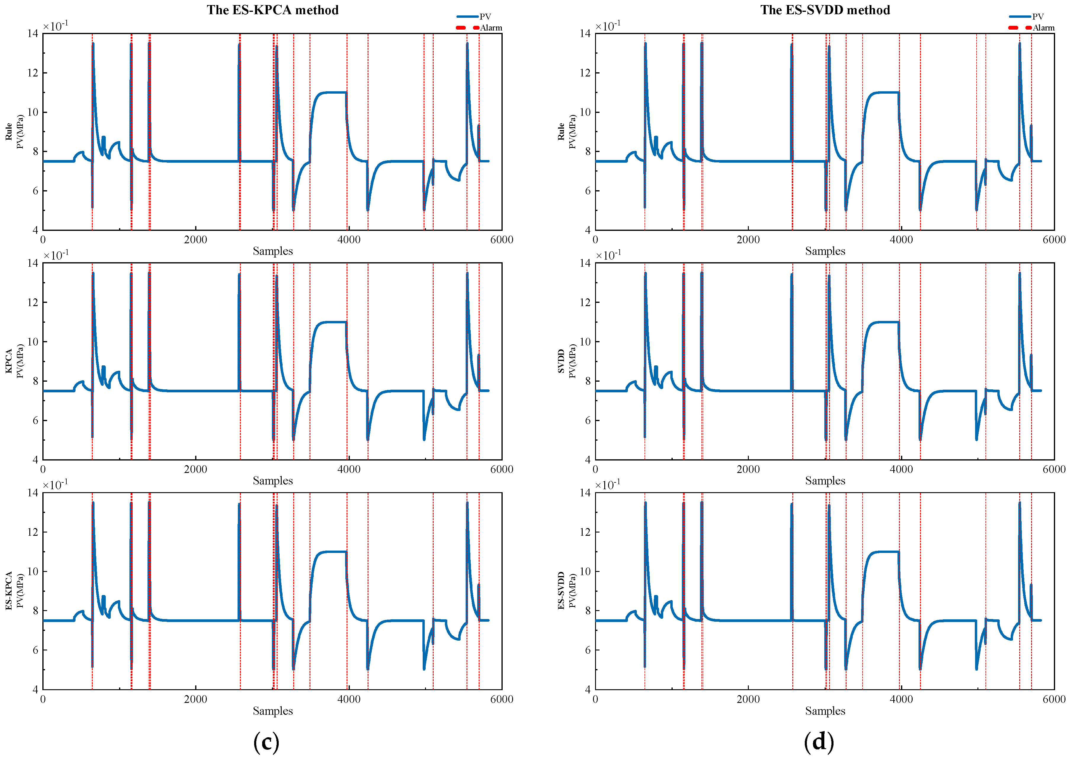
As shown in Figure 6, Figure 7 and Figure 8, all faults in the three process parameters are diagnosed by both methods. In Figure 6 and Figure 8, the alarm positions obtained by the ES-KPCA and ES-SVDD methods are consistent. In Figure 7, during the continuous fluctuations observed from samples 2219 to 2531, the ES-KPCA method triggers 10 alarms, while the ES-SVDD method triggers 1 alarm. At sample 7300, the ES-KPCA method triggers two alarms, while the ES-SVDD method does not trigger an alarm due to the anomalies observed at samples 6923 and 6935. Thus, the ES-KPCA method emphasizes real-time alarms, while the ES-SVDD method focuses on the first alarm, which has been validated. Additionally, at sample 3707, the ES-SVDD method exhibits a slight false alarm due to minor operational adjustments. The forward time series judgment data matrix is relatively stable, resulting in a smaller radius of the constructed hypersphere, and the diagnosis vector lies outside the hypersphere.

Table 2. The threshold parameter settings for the ES-KPCA method in UniSim.

Process Parameters	$\mathit{\omega }$	s	k	$\mathit{\theta }$
FIC1013.PV	0.10	2.00	2	2500.00
LIC1506.PV	0.10	2.00	3	15.00
PIC1411.PV	0.05	2.00	2	0.50

and

Table 3. The threshold parameter settings for the ES-SVDD method in UniSim.

Process Parameters	$\mathit{\omega }$	$\mathit{\xi }$	s	C
FIC1013.PV	0.10	1.00	5.00	0.20
LIC1506.PV	0.10	1.20	3.00	0.50
PIC1411.PV	0.05	1.00	6.00	0.50

present the offline parameter adjustment results for the ES-KPCA and ES-SVDD methods.

4.3.2. The Online Diagnosis Phase in UniSim

In the online diagnostic phase, the relevant parameters obtained from the offline threshold parameter adjustment phase in Table 2 and Table 3 are acquired for the ES-KPCA and ES-SVDD methods. The three process parameters were diagnosed online 444 times, with 5920 real-time data samples being collected. For comparison purposes, the KPCA method and the SVDD method were replaced with the PCA method and the OCSVM method, respectively, resulting in the expert system for the process parameter trend anomaly diagnosis based on rolling data PCA and OCSVM (ES-PCA and ES-OCSVM). The similarity thresholds for the ES-PCA and ES-OCSVM methods were denoted as $\gamma$ and $\epsilon$, respectively. Other relevant threshold parameters remained the same for both methods. The detailed parameter configurations are presented in

Table 4. The threshold parameter settings for the ES-PCA and ES-OCSVM methods in UniSim.

Process Parameters	Method	$\mathit{\gamma }$	$\mathit{\epsilon }$
FIC1013.PV	ES-PCA	2000.00
	ES-OCSVM		0.40
LIC1506.PV	ES-PCA	60.00
	ES-OCSVM		3.00
PIC1411.PV	ES-PCA	0.22
	ES-OCSVM		8.00

.

The fault settings are shown in

Table 5. Fault settings for online diagnosis of relevant process parameters in UniSim.

Process Parameters	Fault Configuration	Times
FIC1013.PV	Large amplitude pulses	10
	Large amplitude process adjustments	2
	Small amplitude process adjustments	11
LIC1506.PV	Large amplitude pulses	11
	Large amplitude process adjustments	3
	Significant progressive adjustments	2
	Small amplitude process adjustments	6
PIC1411.PV	Large amplitude pulses	9
	Large amplitude process adjustments	2
	Small amplitude process adjustments	8

, and the diagnostic results are shown in Figure 9, Figure 10 and Figure 11.

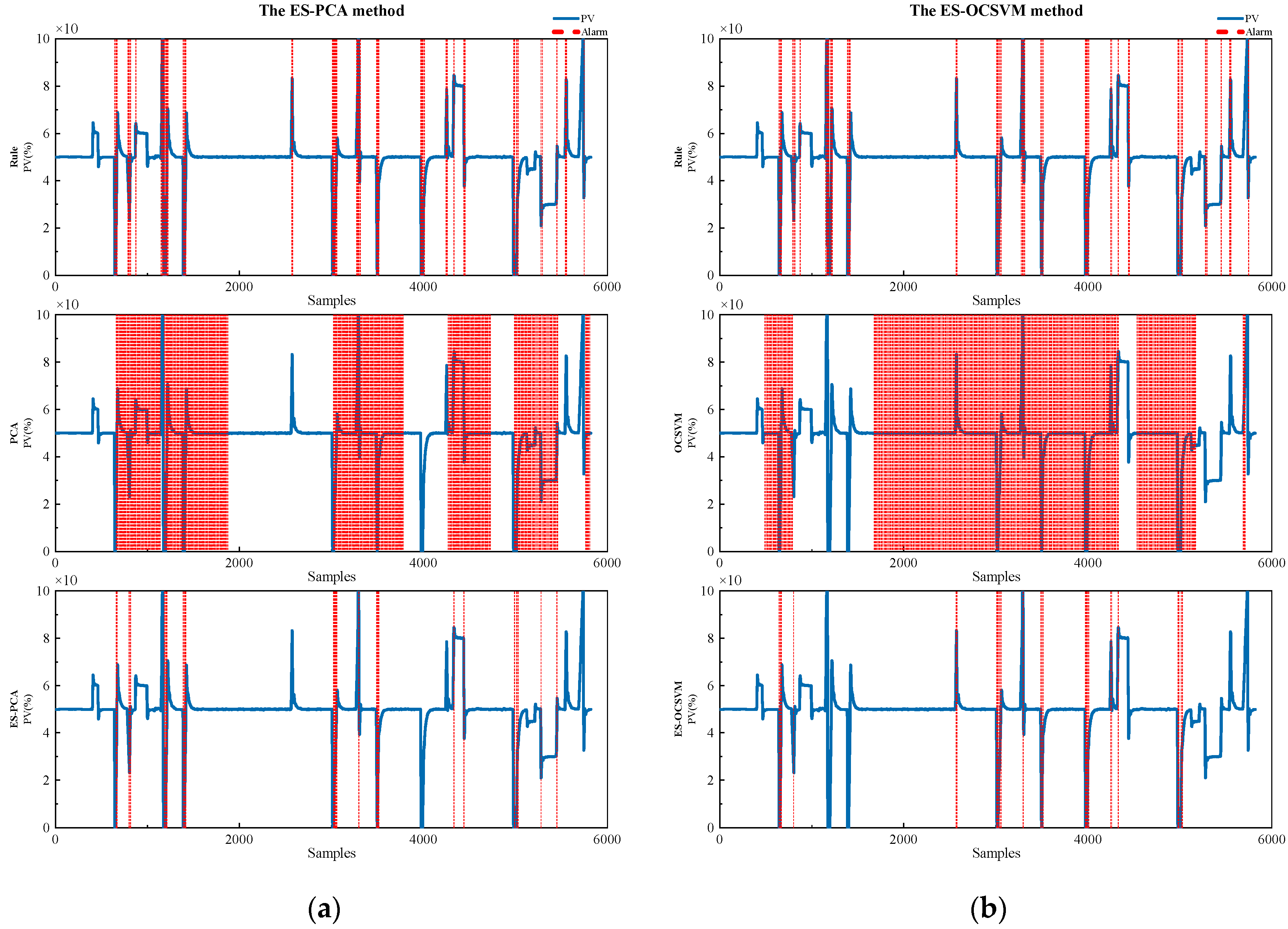
In Figure 9a, the rolling data PCA method exhibits excessive false positives. Under the rule specified by the expert system, the ES-PCA method detected 9 out of 10 for large amplitude pulses and 1 missed detection; 2 large amplitude process adjustments were detected, but there were 3 false alarms for small amplitude process adjustments, indicating a relatively bad diagnostic performance. In Figure 9b, the rolling data OCSVM method generates multiple false positives between samples 491 and 1451. However, after applying the specified rule, the ES-OCSVM method detected 9 out of 10 large amplitude pulses and 1 missed detection; 2 large amplitude process adjustments were detected, but there was 1 false alarm for small amplitude process adjustments, indicating a moderate diagnostic performance. Figure 9c,d shows that the ES-KPCA method triggered 22 alarms, while the ES-SVDD method triggered 24 alarms. They include all 10 large amplitude pulses and 2 large amplitude process adjustments, without any false alarms for small amplitude process adjustments, indicating an excellent diagnostic performance.

In Figure 10a, the rolling data PCA method shows excessive false positives and missed positives. Under the constraints of the rule, the ES-PCA method detected 8 out of 11 large amplitude pulses and 3 missed detections; 3 large amplitude process adjustments were detected, but there was 1 false alarm for 6 small amplitude process adjustments, and 1 out of 2 significant progressive adjustments were detected with 1 missed detection, indicating a moderate diagnostic performance. In Figure 10b, the rolling data OCSVM method generates too many false positives and some false negatives. The ES-OCSVM method detected 6 out of 11 large amplitude pulses and 5 missed detections, 1 detected for 3 large amplitude process adjustments with 2 missed detections, no false alarms for 6 small amplitude process adjustments, and detected 1 out of 2 significant progressive adjustments with 1 miss, indicating a relatively poor diagnostic performance. Figure 10c,d shows that the ES-KPCA method has a total of 15 alarms, while the ES-SVDD method has a capacity for 36 alarms. Both methods detected all 11 large amplitude pulses, and the ES-SVDD method had more alarms for individual pulses than the ES-KPCA method, which is consistent with the training results. They detected all three large amplitude process adjustments and did not produce any false alarms for six small amplitude process adjustments. For the two significant progressive adjustments, the ES-KPCA method had one alarm and one missed detection, while the ES-SVDD method had two alarms and no missed detections, indicating that the ES-KPCA method’s ability to detect anomalies caused by long-term small trends is weak.

In Figure 11a, the ES-PCA method detected six out of nine large amplitude pulses and three missed detections, two large amplitude process adjustments were detected, and there were no false alarms for eight small amplitude process adjustments. In Figure 11b, the ES-OCSVM method detected six out of nine large amplitude pulses and three missed detections, one detected for two large amplitude process adjustments with one missed detection, and no false alarms for eight small amplitude process adjustments. Figure 11c,d shows that the ES-KPCA and ES-SVDD methods had similar alarm locations, with 15 alarms. They detected all nine large amplitude pulses, two large amplitude process adjustments, and there were no false alarms for eight small amplitude process adjustments, indicating an excellent diagnostic performance.

Due to an excessive number of stable samples in the data of the process parameters, the values of the three evaluation indicators in Equations (24)–(26) are excessively large, making data analysis difficult. To facilitate a better analysis, the following strategies are adopted:

• Defining samples with large amplitude pulses, large amplitude process adjustments, and large amplitude gradual adjustments as negative samples.
• Defining samples with small amplitude process adjustments as positive samples.

The evaluation results of diagnostic performance for the three parameters are shown in

Table 6. The comparative results of three methods for three process parameters.

Process Parameters	Method	Precision	Recall	F1-Score
FIC1013.PV	ES-PCA	0.89	0.73	0.80
	ES-OCSVM	0.90	0.90	0.90
	ES-KPCA	1.00	1.00	1.00
	ES-SVDD	1.00	1.00	1.00
LIC1506.PV	ES-PCA	0.56	0.83	0.67
	ES-OCSVM	0.43	1.00	0.60
	ES-KPCA	0.86	1.00	0.93
	ES-SVDD	1.00	1.00	1.00
PIC1411.PV	ES-PCA	0.73	1.00	0.84
	ES-OCSVM	0.67	1.00	0.80
	ES-KPCA	0.89	1.00	0.94
	ES-SVDD	0.89	1.00	0.94

.

According to Table 6, for the pressure parameter FIC1013.PV, the ES-KPCA method and the ES-SVDD method models have the same F1-score, which is higher than that of the ES-PCA and ES-OCSVM methods. This indicates that the ES-KPCA and ES-SVDD methods have a similar and superior performance compared to the ES-PCA and ES-OCSVM methods. For the level parameter LIC1506.PV, the ES-SVDD method has a higher F1-score than the other three methods, and the ES-KPCA method has a higher F1-score than the ES-PCA and ES-OCSVM methods, indicating that the ES-SVDD method performs the best. For the pressure parameter PIC1411.PV, both the ES-KPCA and ES-SVDD methods have the same F1-score, which is higher than that of the ES-PCA and ES-OCSVM methods, indicating that both the ES-KPCA and ES-SVDD methods are equally good. In summary, for the flow rate and pressure parameters, the ES-KPCA and ES-SVDD methods have a similar diagnostic performance, while, for the level parameter, the ES-SVDD method outperforms the ES-KPCA method.

4.4. Experiment and Validation with Real Data

The data from a domestic refinery for one year were used, and the same comparative experiment as in Section 4.3 was conducted. During the offline threshold parameter adjustment phase, a total of 131,360 diagnoses were performed using 1,576,800 data sets. The parameter tuning results for the ES-KPCA and ES-SVDD methods are presented in

Table 7. The threshold parameter settings for the ES-KPCA method in Chemical Plant.

Process Parameters	$\mathit{\omega }$	s	k	$\mathit{\theta }$
FIC209.PV	0.05	2.00	2	12.00
TIC205.PV	0.03	2.00	3	5.00

and

Table 8. The threshold parameter settings for the ES-SVDD method in Chemical Plant.

Process Parameters	$\mathit{\omega }$	$\mathit{\xi }$	s	C
FIC209.PV	0.05	1.00	6.00	0.50
TIC205.PV	0.03	1.10	5.00	0.50

. The parameter settings for the ES-PCA and ES-OCSVM methods in the comparative experiment are shown in

Table 9. The threshold parameter settings for the ES-PCA and ES-OCSVM methods in Chemical Plant.

Process Parameters	Method	$\mathit{\gamma }$	$\mathit{\epsilon }$
FIC209.PV	ES-PCA	20.00
	ES-OCSVM		15.00
TIC205.PV	ES-PCA	18.00
	ES-OCSVM		20.00

. The results of the parameter tuning are illustrated in Figure 12 and Figure 13.

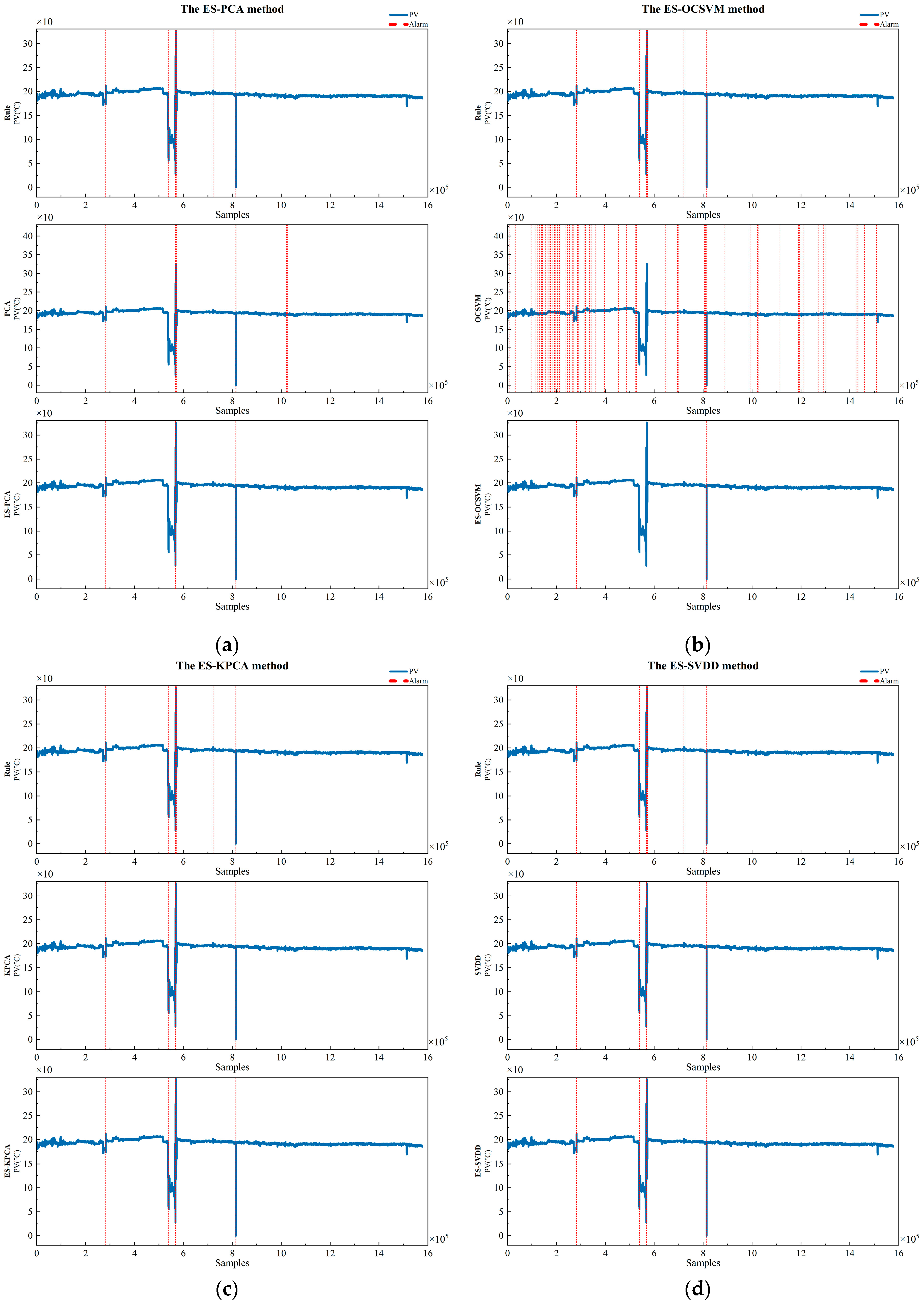
The offline diagnosis results for the process parameter FIC209.PV are shown in Figure 12, where the expert system successfully detects and eliminates the outlier at sample 1,107,680. In Figure 12a, the rolling data PCA method detects all anomalies but suffers from both false positives and discrepancies with rule-based alarms. Consequently, the ES-PCA method misses four occurrences at samples 31,895, 331,955, 515,867, and 719,915 while falsely reporting two instances at samples 789,335 and 1,548,311. In Figure 12b, the rolling data OCSVM and ES-OCSVM methods detect all anomalies, but they also exhibit false positives and discrepancies with rule-based alarms. The ES-PCA method misses six occurrences at samples 27,059, 271,091, 331,955, 515,867, 646,895, and 719,915, while falsely reporting one occurrence at sample 1,548,311. In Figure 12c, the ES-KPCA method has one false negative at sample 331,955. However, in Figure 12d, the ES-SVDD method successfully detects all the anomalies in the trend.

For the process parameter TIC205.PV, the offline training results are shown in Figure 13, where the expert system successfully detects and eliminates the outlier at sample 1,107,680. In Figure 13a, the ES-PCA method has a false negative at sample 540,083, and, in Figure 13b, the OCSVM method exhibits a higher overall false positive rate and also misses some instances. Under the constraints of the rules, the ES-OCSVM method experiences false negatives at samples 540,083 and 569,975. However, in Figure 13c,d, the ES-KPCA and ES-SVDD methods successfully detect all the anomalies in the trend.

In summary, the ES-KPCA and ES-SVDD methods demonstrated a superior performance in process parameter diagnosis, effectively detecting large-scale process adjustments and outliers while avoiding false alarms, showcasing an excellent diagnostic efficacy. In comparison, the ES-PCA and ES-OCSVM methods exhibited relatively less favorable diagnostic outcomes, displaying some instances of missed detections.

5. Conclusions

In order to diagnose the problem of large-scale fluctuations and abnormal trends in process parameters, this paper presents a detailed description of an expert system based on data mining for the trend diagnosis of process parameters. The expert system incorporates a rule-based assessment of process parameter stability to determine whether the process parameters are stable. Moreover, the system uses the rolling data KPCA and SVDD methods to further assess abnormal trends when the parameters are unstable. In this paper, the ES-KPCA method emphasizes the difference between the diagnosis vector and the forward time series judgment data matrix, which is suitable for real-time alarms for online diagnosis. The ES-SVDD method prioritizes the first alarm of online diagnosis, employing the appropriate approach based on the requirement. In addition, an effectiveness validation was conducted using UniSim simulation and data from a domestic refinery, including the flow rate, liquid level, pressure, and temperature process parameters, and comparative experiments were conducted using ES-PCA and ES-OCSVM. The results showed that the expert system proposed in this paper can effectively diagnose large-scale fluctuations and abnormal trends in process parameters, and the detection effect is better than the ES-PCA and ES-OCSVM methods through ablation studies of the expert system. Therefore, the expert system can monitor abnormal changes in process parameters in real-time and take timely action to improve production efficiency and quality levels. It can also be applied to process industries with one-dimensional process parameters in the future. The disadvantage of the expert system is that the hyperparameter values in the expert rules are explicitly set for each process parameter and cannot be processed uniformly.