Adaptive Latin Hypercube Sampling for a Surrogate-Based Optimization with Artificial Neural Network

Abstract

A significant number of sample points are often required for surrogate-based optimization when utilizing process simulations to cover the entire system space. This necessity is particularly pronounced in complex simulations or high-dimensional physical experiments, where a large number of sample points is essential. In this study, we have developed an adaptive Latin hypercube sampling (LHS) method that generates additional sample points from areas with the highest output deviations to optimize the required number of samples. The surrogate model used for the optimization problem is artificial neural networks (ANNs). The standard for measuring solution accuracy is the percent error of the optimal solution. The outcomes of the proposed algorithm were compared to those of random sampling for validation. As case studies, we chose three different chemical processes to illustrate problems of varying complexity and numbers of variables. The findings indicate that for all case studies, the proposed LHS optimization algorithm required fewer sample points than random sampling to achieve optimal solutions of similar quality. To extend the application of this methodology, we recommend further applying it to fields beyond chemical engineering and higher-dimensional problems.

1. Introduction

For many engineering problems, simulation is an essential method to understand the behavior of real systems accurately. In numerous research projects, simulation is employed to interpret complex models, reducing the time and cost associated with real-world process operations. A surrogate model, also known as a meta-model, can be created using a set of input–output data obtained from simulations or experiments. In this context, the simulation is considered a ‘black box,’ where the functions and underlying assumptions of the simulation are unknown except for the process output [1].

The popular surrogate model is Response Surface Methodology (RSM), which is evaluated through the regression of input–output data using low-order polynomials. In recent years, RSM has been applied in several chemical processes to study the effects of independent factors [2,3,4,5,6,7,8]. It has also been used in treatment processes to improve removal efficiency and reduce operating costs [2]. However, for complex processes, low-order polynomials have limitations in capturing highly nonlinear behavior [9]. Generally, RSM provides local optimization results. Therefore, global surrogate models such as Kriging interpolation and artificial neural networks (ANNs) have been proposed to overcome these limitations. Kriging interpolation offers an accurate model that provides better global approximations compared to low-order polynomial models. It predicts output values at specific inputs that match the simulated output values [10]. Kriging interpolation fits a spatial correlation function to a set of input–output pairs, and the data points are used in linear interpolation [11]. However, it is important to note that this surrogate model may have limitations due to available support software. Several surrogate models have been used in the past years, including artificial neural networks (ANNs), radial basis function (RBF), and random forest (RF) [12]. ANNs are a powerful tool for various applications, such as approximating nonlinear systems, process modeling, and optimization [13]. They can fit many complex nonlinear functions and apply to numerous processes in chemical engineering [14,15]. ANNs were coupled with another machine learning technique such as the genetic algorithm [16,17] and simulated annealing [17,18] for application in the engineering process. ANNs are commonly employed due to their simplicity and ability to handle challenging nonlinear mappings [19]. These mathematical models have been used in both laboratory [20,21] and industry [14,22,23]. In 2020, Tahkola et al. developed a surrogate model for electrical machine torque using grid sampling combined with ANNs, and the results demonstrated the effectiveness of this sampling approach in modeling torque behavior [24]. Many studies have shown that ANNs can provide accurate models for various engineering disciplines [25,26,27,28,29,30]. Therefore, ANNs were employed to develop accurate models for the chemical process case studies in this work.

To build a model that describes the relationship of any input and output, the sampling technique is also required to construct the experiment and points of any responses. In order to generate the sample points, the design of experiment (DoE) approach is necessary. Therefore, the study of design of experiment (DoE) is necessary in order to select the numbers and locations of sample points. The development of modern DoE techniques can be categorized into two types, which are static and adaptive [31]. Factorial design, Latin hypercube sampling, the Monte Carlo method and orthogonal array are classified as static DoEs. Factorial design is widely used due to its simplest form of space-filling design, which covers most of the considered regions of variables [32,33]. The first modern design of experiment is Monte Carlo or random sampling, which generates sample points in the design space using random numbers. This technique requires a large number of sample points to represent the entire problem space. Subsequently, Quasi-Monte Carlo was introduced to achieve a uniform distribution of sample points across the design space by using low-discrepancy sequences. Three popular quasi-random low-discrepancy sequences are Halton, Hammersley, and Sobol sequences. However, these sampling techniques, including random sampling, demand a large sample size to achieve a highly accurate model, which results in high costs and time consumption during real process operations. Therefore, the proposed Latin hypercube sampling was studied to address these challenges. Latin hypercube sampling exhibits a beneficial property known as optimum non-collapsing. However, generating Latin hypercube sample points presents challenges, particularly in terms of achieving uniform distribution across the design space. Additionally, in high-dimensional problems, a large number of sample points is needed to adequately cover the design space.

Therefore, this work introduced adaptive Latin hypercube sampling to employ the necessary sample points for representing the design space in simulation-based optimization. The algorithm’s objective is to generate the fewest sample points while achieving the best feasible optimal solution. The algorithm started with a small number of sample points from Latin hypercube sampling. Additional sample points were then generated and sequentially added to an original dataset. Artificial neural networks (ANNs) were employed as a surrogate model. The optimal results obtained from the proposed algorithm were compared with those obtained from random sampling. Three chemical processes were used as case studies to represent problems with varying complexity and numbers of factors. Three replications of each case study were conducted to assess the consistency of the method.

This paper is organized as follows: Section 2 provides reviews of Latin hypercube sampling, random sampling, and artificial neural networks. Section 3 presents the proposed adaptive Latin hypercube sampling for surrogate-based optimization. Section 4 introduces details of three different case studies: (1) ammonia production from syn gas, (2) methanol production via CO₂ hydrogenation, and (3) CO₂ capture using the Rectisol process to represent three different types of surrogate-based optimization problems. Section 5 offers results, discussion, recommendations, and future work. Finally, Section 6 presents the conclusion.

2. Sampling Technique and Surrogate Modeling

This section provides information on sampling techniques and surrogate models. Section 2.1 describes Latin hypercube sampling, Section 2.2 provides information on random sampling, and Section 2.3 describes the artificial neural network.

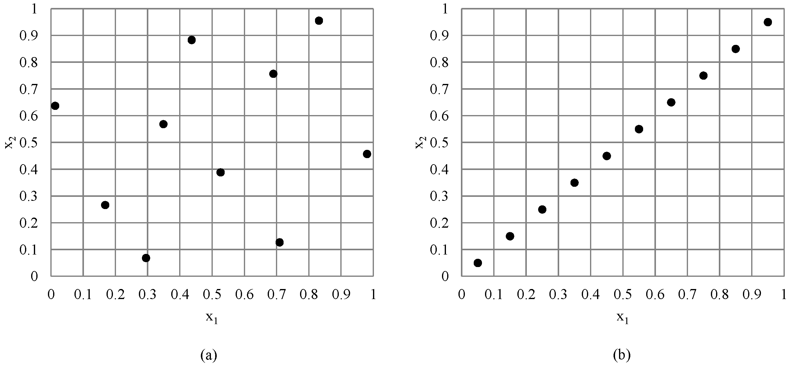
2.1. Latin Hypercube Sampling

Latin hypercube sampling was first proposed in 1979 by M.D. Mckey et al. [34]. It is a method for generating samples that cover the entire sample space without any replications. The technique involves dividing each dimension of the sample space into N equally likely intervals for N sample points. The fundamental principle of Latin hypercube sampling is to ensure that each stratum is sampled exactly once, thereby guaranteeing a comprehensive representation of the entire sample space. For instance, in Latin hypercube sampling (LHS) involving two factors and ten sample points, the range of each factor, typically from 0 to 1, is partitioned into ten equal intervals. Each sample point is then randomly chosen from one of these intervals, creating a distinctive and stratified LHS dataset. Each interval accommodates only one sample point, which is randomly paired with other variables. You can observe this LHS dataset in Figure 1a.

One advantage of Latin hypercube sampling (LHS) is that by selecting input points independently, it ensures that the sampled points are spread across the entire parameter space without clustering in any particular region. This reduces the risk of overemphasizing certain areas of the space, which can occur with other random sampling methods. Moreover, LHS ensures that once a point is sampled, it will not be selected again. This feature minimizes redundancy in the samples, allowing the system to focus on exploring new regions of the parameter space, leading to different output results. The illustration of Latin hypercube sampling is shown in Figure 1. However, the worst-case scenario for Latin hypercube sampling may result in poorly sampled spaces, as depicted in Figure 1b, which may not adequately represent the entire domain space. Therefore, in any field that uses Latin hypercube sampling as a sampling technique for optimization problems, it is essential to ensure that samples cover the entire parameter space (space filling).

To address the primary challenge in Latin hypercube sampling, researchers have explored various criteria to generate well-filling Latin hypercube designs, aiming to enhance their performance.

Table 1. The approach for constructing optimal Latin hypercube sampling.

Algorithm	Criteria	Pros.	Cons.
Simulated annealing [36,37,38]	Maximize the inter-point distance	Effective for small-size problems	Converge very slowly
Exchange type and Newton type [39]	Maximize entropy	Fast to find optimal design for large-size problems
Columnwise–pairwise [40]	Maximize the inter-point distance and Maximize entropy	Retain some orthogonality and high efficiency for small designs	Does not significantly reduce the searching time
Threshold accepting [41]	Minimize L2 discrepancy	Can be applied to both factorial and computer experiment	Cannot give a good design for small dimension
Genetic algorithm [42]	Maximize the inter-point distance	Requires a small amount of computational time
Enhanced stochastic evolutionary algorithm [43]	Maximize the inter-point distance, maximize entropy and minimize L2 discrepancy	Needs a small number of exchanges; effective for large-size problems
Branch-and-bound [44]	Maximize the inter-point distance	Can be used for non-collapsing designs	Obtain the optimum design for N < 70
Translational propagation [45]	Maximize the inter-point distance	Obtain near-optimum LHDs up to medium dimensions	High computational cost for large number of sample points
Particle swarm optimization [46,47]	Maximize the inter-point distance	Fast accessibility to reach solutions	Local search algorithms become trapped in local optima
Translational propagation [48]	Maximize the inter-point distance and minimize L2 discrepancy	Effective in terms of the computation time and space-filling and projective properties	Not good in terms of performance of sampling points
Enhanced stochastic evolutionary algorithm [49]	Maximize the inter-point distance	Effective for large-size problems

summarizes the criteria used in Latin hypercube sampling. The two most common criteria used in Latin hypercube sampling (LHS) involve maximizing the minimum inter-point distance between pairs of sample points and minimizing the correlation between pairs of columns in the sample matrix [35]. By maximizing the minimum distance, LHS avoids the problem of points clustering in certain regions of the parameter space. Clustering can lead to bias in estimation and might cause important regions of the space to be overlooked. By minimizing the correlation between pairs of columns in the LHS matrix, it ensures that the selected variables or factors are as orthogonal as possible. This means that the variables are as independent as possible, and each factor has less influence on the others. This makes it easier to identify the individual impact of each variable on the system’s output. However, when dealing with a large number of sample points or when integrating them with the optimization of a specific case study, these algorithms may require more computational time and become complex.

In order to reduce computational time, the adaptive Latin hypercube with sequential design is an intriguing choice for case studies involving process simulation. Adaptive sampling strategies typically begin with a small sample size and then sequentially add points based on specific criteria. In 2003, Wang proposed an adaptive response surface methodology model using inherited Latin hypercube sampling points [50]. This sampling approach involves adding new sample points in underrepresented areas. Subsequently, in 2018, Chang applied this technique instead of central composite design to calculate the failure probability of a complex turbine blade structure [51]. The results demonstrated the effectiveness of this approach when combined with Gaussian process regression for structural reliability analysis. Another variation of adaptive Latin hypercube sampling, which initially identifies the region of interest, was introduced by Roussouly [52]. After marking the location and sampling the first point, the region is subdivided to add two more sample points. Finally, two additional sample points are introduced using another two-point Latin hypercube. This technique offers advantages for reliability analysis by focusing sampling efforts solely on the areas of interest. Zhi-zhao Liu and colleagues proposed two general extension algorithms for Latin hypercube sampling: basic general extension and general extension based on the greedy algorithm [53]. These algorithms aim to preserve the majority of the original Latin hypercube points. While the general extension approach can be time consuming, the general extension based on the greedy algorithm reduces computational time, though it may lead to the removal of some of the original points. In 2016, a rigorous Latin hypercube sampling method was coupled with a sophisticated algorithm to ensure the retention of all initial points [54].

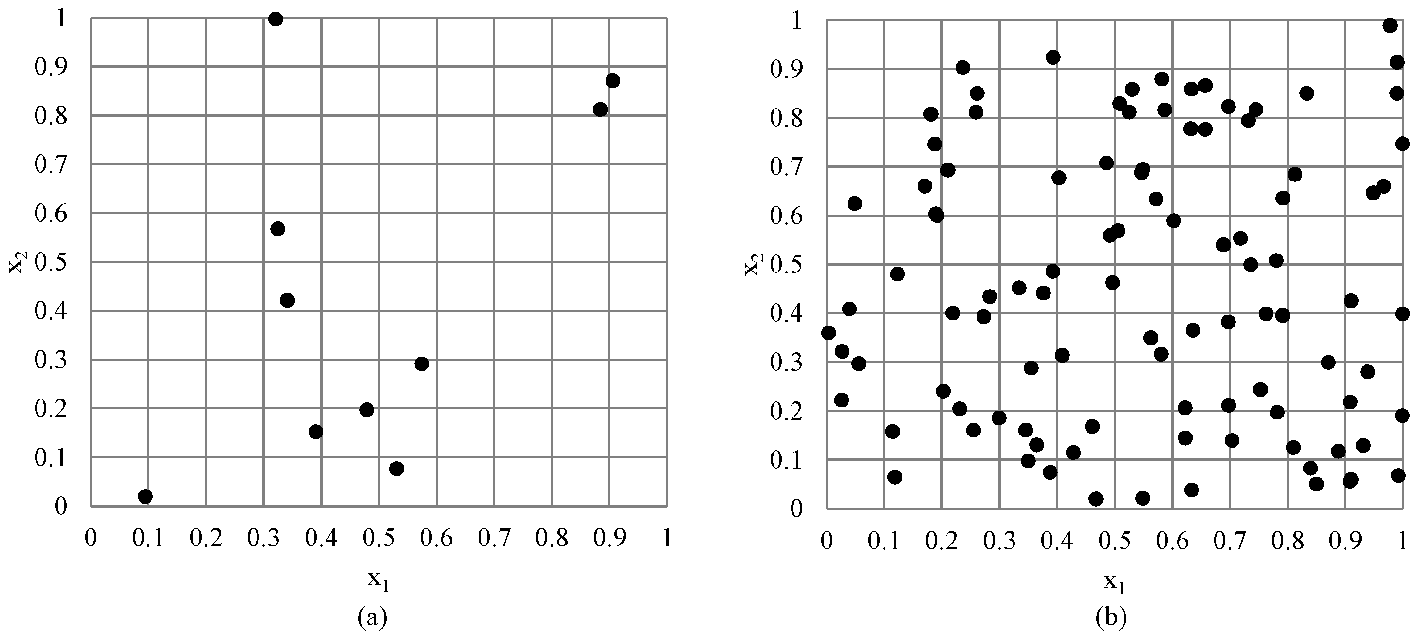
2.2. Random Sampling

Monte Carlo or random sampling was the first modern sampling design for computer experiments, which was proposed by Metropolis and Ulam in 1949 [55]. Random sampling requires a large number of sample points (N) to achieve a high level of accuracy in surrogate modeling. However, this approach consumes more computational time and is time consuming in terms of data collection. Figure 2 illustrates random sampling.

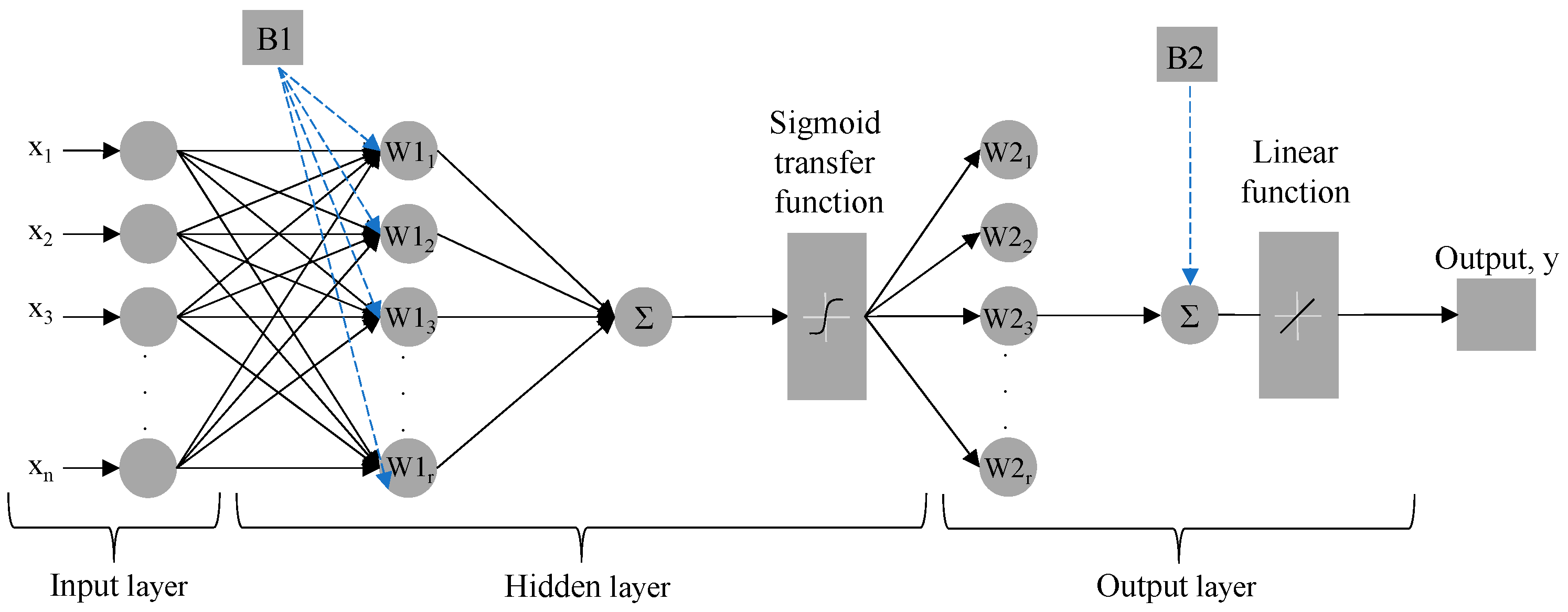
2.3. Artificial Neural Networks (ANNs)

Artificial neural networks are mathematical expressions consisting of interconnected processing units known as neurons. These computer systems mimic the biological neural networks found in animals. The parameters of the network include weights and biases. Each neuron operates by using a transfer function. Generally, feedforward neural networks are widely used for mathematical expressions, forming a directed graph. The primary structure of artificial neural networks includes an input layer, a hidden layer, and an output layer.

In this research, a three-layer feedforward neural network was used to train the dataset due to its mathematical simplicity. Figure 3 illustrates the schematic of the feedforward neural network with a single hidden layer.

The training algorithm includes Levenberg–Marquardt, Bayesian regularization, and scaled conjugate gradient techniques. However, Levenberg–Marquardt requires less time than the others [56]. The input for the ANNs consists of a dataset of operational and design parameters, which was generated using the original Latin hypercube sampling. The output of the ANNs is the predicted cost corresponding to each process. In terms of neural network hyperparameters in this research, a single hidden layer with eight neurons was employed in the ANN network. The sigmoid function is used to model the relationship between the input and the hidden layer. It is smooth and differentiable everywhere, making it suitable for gradient-based optimization methods such as backpropagation. The smoothness of activation functions ensures that small changes in weights and biases result in continuous changes in the output, which is crucial for efficient training. The mathematical equations corresponding to the weights and biases of ANNs used to estimate the output (y) are shown in Equations (1) and (2).

$$y=\left({\displaystyle \sum _{r}W{2}_r\times L_r}\right)+B2$$

(1)

$$L_r=\frac{2}{1+e^{-2\left({\displaystyle \sum _r\left(W{1}_{r,k}\times x_{k,r}\right)}+B{1}_r\right)}}$$

(2)

where k is the number of decision variables, r is the number of neurons in a hidden layer, and W1 and W2 are input weights of the hidden layer and output layer, respectively. The parameters B1 and B2 are biases of the input and the output layers, respectively.

3. Methodology

The methodology of this work is divided into three sections. In Section 3.1, we introduce the adaptive Latin hypercube sampling approach for surrogate-based optimization, which focuses on solving optimization problems using a small set of sample points. The algorithm’s optimal solutions are validated through outcomes obtained via random sampling. Section 3.2 covers the details of adaptive LHS in the proposed surrogate-based optimization, while Section 3.3 offers detailed insights into optimization using random sampling. Adaptive Latin hypercube sampling is a sequential sampling method that increases the number of sample points one by one until it meets the algorithm’s criteria. In contrast, random sampling is a one-time operation that generates the entire set of sample points at once without the option to add more. In this work, if the number of sample points in random sampling cannot adequately represent the entire surface, the algorithm will generate a new initial dataset with twice the number of sample points as in the previous set.

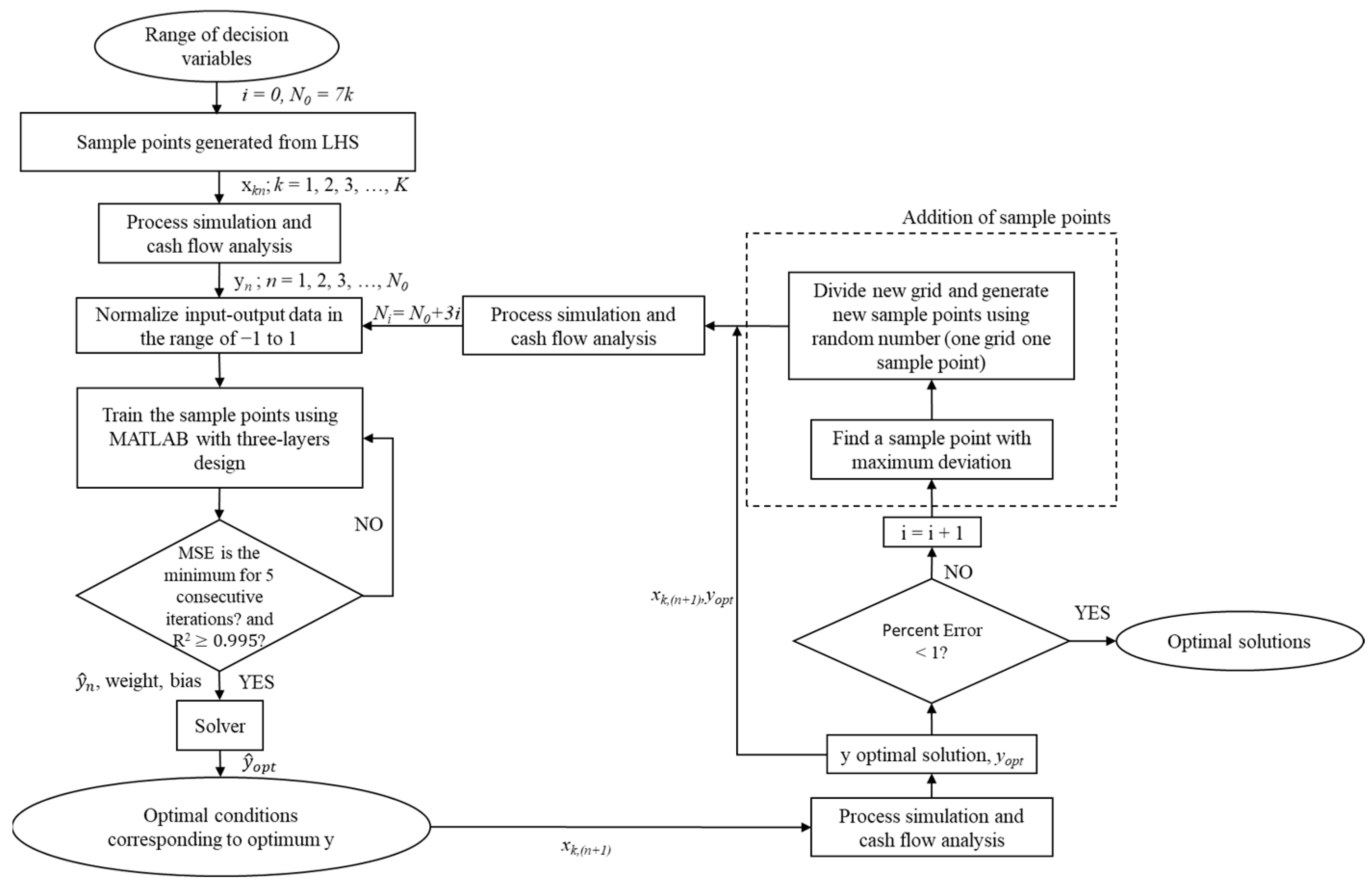
3.1. Proposed Adaptive LHS for Surrogate-Based Optimization Algorithm

Figure 4 represents the proposed adaptive Latin hypercube sampling for surrogate-based optimization. At the beginning of the algorithm, ranges of factors that have effects on the output value were assigned. Then, the first dataset of x_kn (with the desired number of sample points) was generated using Latin hypercube sampling where k = 1, 2, 3, …, K and n = 1, 2, 3, …, N₀, (K is number of decision variables, and N is number of sample points). The initial number of sample points was set at seven times the number of factors. The corresponding output values, y_n, were obtained from process simulation combined with an economic analysis. The sets of input and output were normalized in the range of −1 to 1 for ANNs training using MATLAB with a three-layer design (input layer, hidden layer, and output layer).

For ANNs training, the Levenberg–Marquardt algorithm was used. The dataset was split into 70% for training, 15% for validation, and 15% for testing. The criteria used to determine the accuracy of the ANN model are the mean square error (MSE) [57] and the R-squared (R²) value. The training loop for ANNs was terminated when the MSE value of the ANN model remained at a minimum for 5 consecutive iterations, and the R² value of the model was greater than or equal to 0.995. The weights and biases of the most recent ANN model were then used as the objective function for the optimization problem to determine the optimal solution (x_i,opt and ${\widehat{y}}_{opt}$). The optimal operating conditions (x_i,opt) were then input into the process simulation to obtain the corresponding output value (y_opt). The accuracy of the obtained optimal solution is deemed acceptable if the percent error between the predicted output value (obtained from the ANN model) and the actual output value (obtained from process simulation), as shown in Equation (3), is within a preset value of 1 percent. If the percent error is less than one, the optimization algorithm is terminated, and the most recent optimal solution is reported as the optimal solution of the problem.

If the percent error value exceeds one, three additional data points are incorporated into the existing dataset. The first additional data point is the most recent optimal solution (x_i,opt, y_opt), while the other two data points are generated using the adaptive Latin hypercube sampling method (as described in Section 3.2). The updated dataset was then normalized, and these steps were repeated until the percent error in the output falls below one, ultimately yielding the optimal solution.

$$\mathrm{Percent}\mathrm{error}=\frac{\left|y_{n+1}-{\widehat{y}}_{n+1}\right|}{y_{n+1}}\times 100$$

(3)

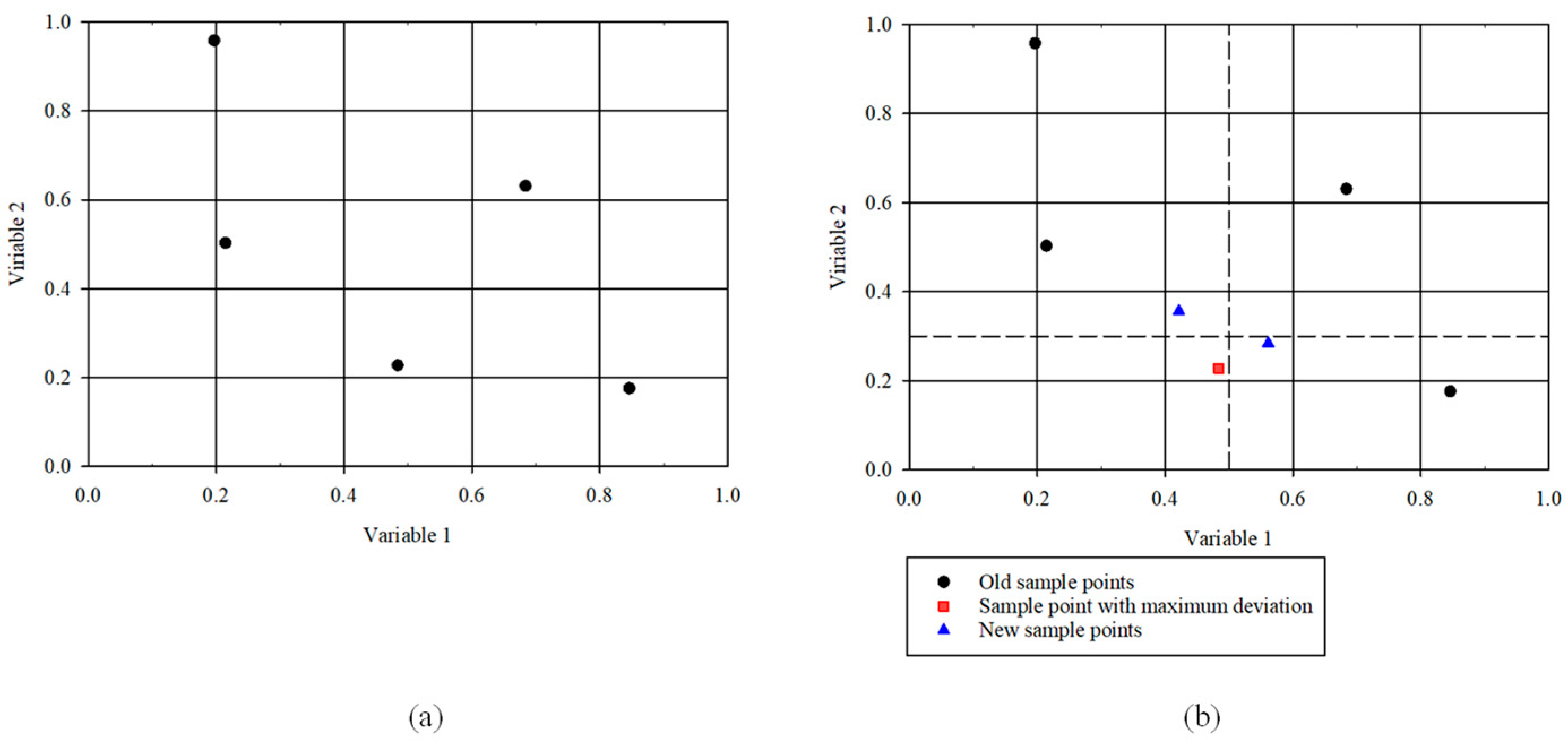
3.2. Adaptive Latin Hypercube Sampling: Addition of Sample Points

In the step involving the addition of sample points in adaptive LHS, two additional sample points are generated during each iteration. To determine these sample points, the deviation from their respective actual values for all (N₀ + 3i) predicted outputs is calculated for each sample point in the dataset, where i represents the number of iterations. The sample point that exhibits the highest deviation, denoted as (x_n, y_{n,max deviation}), is selected. Subsequently, the intervals corresponding to the sample point with the highest deviation (x_n, y_{n,max deviation}) are evenly divided into two intervals. Two additional sample points are then randomly selected from each of these intervals.

Figure 5 illustrates an example of generating two additional sample points from the highest deviation output sample point. This example showcases the generation of sample points for two factors, which are denoted as x₁ and x₂. The highest deviation sample point (x_n, y_{n,max deviation}) is represented as a red dot. The intervals corresponding to these sample points are within the ranges of 0.4 to 0.6 for factor 1 and 0.2 to 0.4 for factor 2. Both factors are evenly divided into two intervals: 0.4 to 0.5 and 0.5 to 0.6 for factor 1, and 0.2 to 0.3 and 0.3 to 0.4 for factor 2 (as indicated by dashed lines). Next, one sample point is randomly selected from each interval of the factors. A total of two additional sample points are obtained and represented as blue dots.

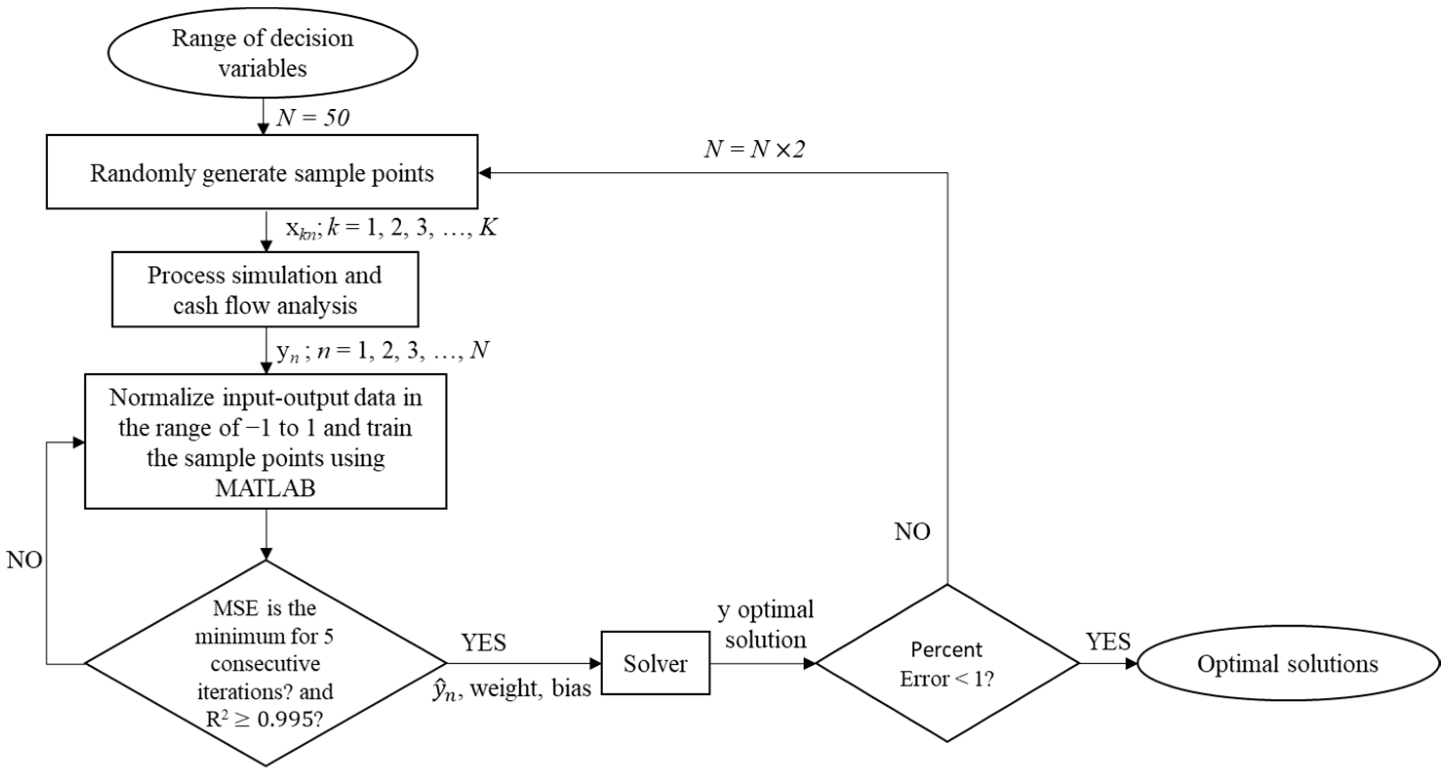
3.3. Verification of the Optimal Solution Using Random Sampling Technique

Figure 6 illustrates the simulation–optimization algorithm using the random sampling technique. The algorithm commenced with the same input ranges and factors as the proposed simulation–optimization method employing adaptive LHS. Initially, 50 sample points were used. Output data were collected, and ANNs were trained using the same stopping criterion as in the proposed method. The resulting ANN model was then subjected to optimization using a nonlinear solver to obtain the optimal solution. The accuracy of the optimal solution was evaluated using the same criteria as in the proposed algorithm. The algorithm terminated and reported the optimal solution if the percent error of the solution was less than one. If not, additional points were generated and added to the original samples, doubling the recent sample size (N × 2). These additional points were then processed through the simulation, and the steps were repeated until the determined optimal solution achieved a percent error of less than one.

4. Case Study

To illustrate the varying complexity and number of factors in the problem, this section examines three distinct chemical processes as case studies. Case Study I focuses on ammonia production from syngas, which involves three factors. Case Study II explores methanol production via carbon dioxide hydrogenation, which deals with four factors. Case Study III addresses CO₂ absorption by methanol using the Rectisol process, which involves five factors. The details of each case study are provided below.

4.1. Process Simulation and Economic Evaluation

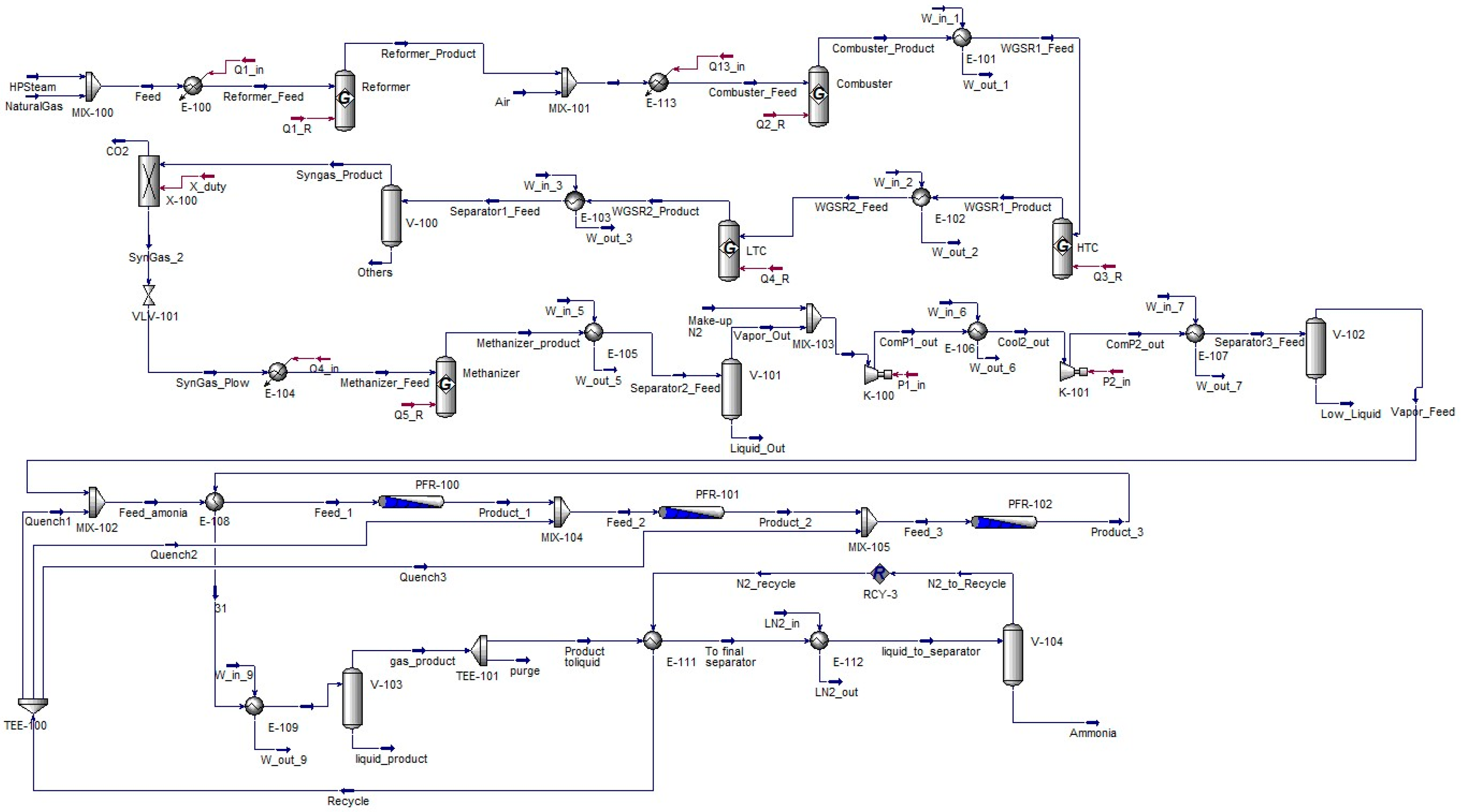
4.1.1. Case Study 1: Ammonia Production from Syngas

The first case study addresses an optimization problem with three decision variables. Figure 7 depicts the process simulation of ammonia production based on the Haber process. The process involves feeds of 31,900 kg per hour of natural gas at 35 bar and 25 °C as well as 95,800 kg per hour of high-pressure steam at 150 bar. Further details on the process simulation and conditions can be found in the work of Janosovsky [58]. Ammonia production comprises two main parts: the production of syngas and the production of ammonia (Equation (16)). The syngas production includes steps such as steam reforming (Equations (4)–(7)), air reforming (Equations (9)–(12)), high and low shift conversion (Equation (13)), CO₂ removal, and methanation (Equations (14) and (15)). The reactions for each step are as follows.

Steam reforming (Reformer unit)

$${\mathrm{CH}}_4+{\mathrm{H}}_2\mathrm{O}\hspace{1em}\to \hspace{1em}\mathrm{CO}+3{\mathrm{H}}_2$$

(4)

$${\mathrm{C}}_2{\mathrm{H}}_6+2{\mathrm{H}}_2\mathrm{O}\hspace{1em}\to \hspace{1em}2\mathrm{CO}+5{\mathrm{H}}_2$$

(5)

$${\mathrm{C}}_3{\mathrm{H}}_8+3{\mathrm{H}}_2\mathrm{O}\hspace{1em}\to \hspace{1em}3\mathrm{CO}+7{\mathrm{H}}_2$$

(6)

$${\mathrm{C}}_4{\mathrm{H}}_8+4{\mathrm{H}}_2\mathrm{O}\hspace{1em}\to \hspace{1em}4\mathrm{CO}+9{\mathrm{H}}_2$$

(7)

Air reforming (Combuster unit)

$$2\mathrm{CO}+{\mathrm{O}}_2\hspace{1em}\to \hspace{1em}2{\mathrm{CO}}_2$$

(8)

$$2{\mathrm{H}}_2+{\mathrm{O}}_2\hspace{1em}\to \hspace{1em}2{\mathrm{H}}_2\mathrm{O}$$

(9)

$${\mathrm{CH}}_4+2{\mathrm{O}}_2\hspace{1em}\to \hspace{1em}2{\mathrm{H}}_2\mathrm{O}+{\mathrm{CO}}_2$$

(10)

$$2{\mathrm{CH}}_6+7{\mathrm{O}}_2\hspace{1em}\to \hspace{1em}6{\mathrm{H}}_2\mathrm{O}+4{\mathrm{CO}}_2$$

(11)

$${\mathrm{C}}_3{\mathrm{H}}_8+5{\mathrm{O}}_2\hspace{1em}\to \hspace{1em}4{\mathrm{H}}_2\mathrm{O}+3{\mathrm{CO}}_2$$

(12)

Water gas shift reaction (HTC and LTC units)

$$\mathrm{CO}+{\mathrm{H}}_2\mathrm{O}\hspace{1em}\leftrightarrow \hspace{1em}{\mathrm{CO}}_2+{\mathrm{H}}_2$$

(13)

Methanation (Methanizer unit)

$$\mathrm{CO}+3{\mathrm{H}}_2\hspace{1em}\leftrightarrow \hspace{1em}{\mathrm{CH}}_4+{\mathrm{H}}_2\mathrm{O}$$

(14)

$${\mathrm{CO}}_2+4{\mathrm{H}}_2\hspace{1em}\leftrightarrow \hspace{1em}{\mathrm{CH}}_4+2{\mathrm{H}}_2\mathrm{O}$$

(15)

Ammonia production (PFR-100, PFR-101 and PFR-102 units)

$${\mathrm{N}}_2+3{\mathrm{H}}_2\hspace{1em}\leftrightarrow \hspace{1em}2{\mathrm{NH}}_3$$

(16)

For the process optimization, three decision variables are the reformer temperature, the combuster temperature, and the low-temperature conversion reactor temperature. The ranges of these decision variables are shown in

Table 2. Range of decision variables of Case Study 1.

Decision Variables	Range
Reformer temperature (°C)	900 to 1200
Combuster temperature (°C)	1400 to 1700
Low-temperature conversion reactor temperature (°C)	160 to 290

. The temperatures of the high-temperature conversion reactor, methanizer, and ammonia reactor were fixed at 450 °C, 340 °C and 450 °C, respectively. A two-stage compressor was used to increase the pressure of the stream up to 150 bar before entering the ammonia synthesis loop. The ammonia synthesis system was modeled using three plug flow reactors in series with three quenching sections. The final product, ammonia, was separated by a separation unit at 45 °C with ammonia content exceeding 98 mol%. More details for replicating the process simulation are provided in Supplementary Information S1.1.

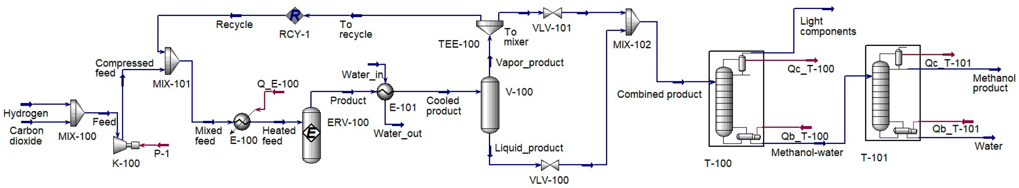
4.1.2. Case Study 2: Methanol Production via Carbon Dioxide Hydrogenation

The second case study represents an optimization problem with four decision variables. Figure 8 depicts the process simulation of methanol production via carbon dioxide hydrogenation with a recycling process. The decision variables were (1) pressure of the equilibrium reactor, (2) temperature of the equilibrium reactor, (3) temperature of the steam entering a separator, and (4) the recycle ratio. This simulation used the Peng–Robinson thermodynamics package. The feed stream of the process consisted of 1000 kmole per hour of carbon dioxide and 3000 kmole per hour of hydrogen at conditions of 20 bar and 40 °C. The process’s specification was to achieve a methanol product purity of 99.5% by mole. The range of each decision variable is shown in

Table 3. Range of decision variables of Case Study 2.

Decision Variables	Range
Pressure of the equilibrium reactor (bar)	50 to 70
Temperature of the equilibrium reactor (°C)	190 to 210
Temperature of the steam entering a separator (°C)	60 to 80
Recycle ratio	0 to 1

. Details of the economic evaluation assumptions for this process can be found in the work of Borisut and Nuchit-prasittichai [57]. Additional information for reproducing the process simulation is provided in Supplementary Information S1.2.

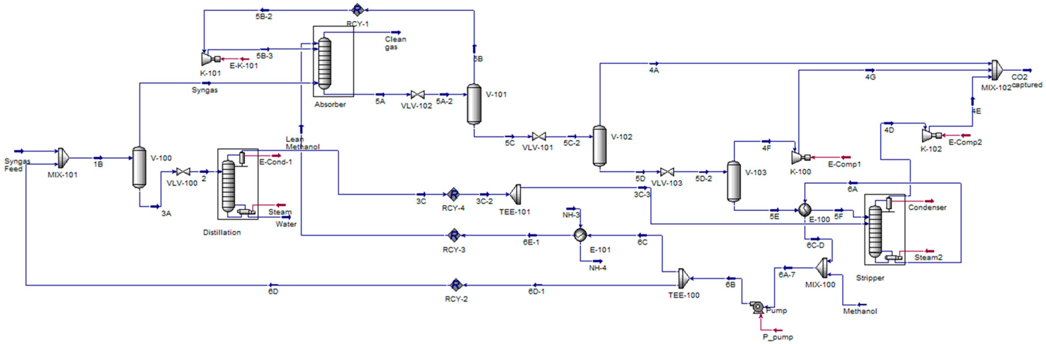
4.1.3. Case Study 2: Methanol Production via Carbon Dioxide Hydrogenation

The third case study represents an optimization problem with five decision variables. Figure 9 illustrates the process of CO₂ absorption by methanol via the Rectisol process. The process consists of three main sections: water removal, absorption, and CO₂/methanol separation. The syngas feed contains a mole fraction of 0.2462 of CO₂, 0.0002 of NH₃, 0.0044 of CO, 0.0050 of Ar, 0.4148 of N₂, 0.3186 of H₂, 0.0035 of H₂O, and 0.0073 of CH₄ at 17.24 bar and 18.30 °C [59]. A small amount of methanol was mixed with the syngas feed and sent to the first separator to separate water from the feed gas. Subsequently, the syngas was fed to an absorber column, where CO₂ gas was captured by chilled methanol added at the top of the column. The rich methanol then passes through a three-stage separator and is fed into a stripper column to separate CO₂ from methanol. The lean methanol leaving the stripper was mixed with 40 kmole per hour of makeup methanol and recycled to the absorber. The vapor product from the stripper, primarily containing CO₂, was combined to other CO₂ product streams from the second and third separators. Details for replicating the process simulation are provided in Supplementary Information S1.3.

In the optimization of this process, the decision variables included the lean methanol temperature, the third-stage separator pressure, the stripper reflux ratio, the stripper inlet temperature, and the distillation reflux ratio. The ranges of these decision variables are detailed in

Table 4. Range of decision variables of Case Study 3.

Decision Variables	Range
Lean methanol temperature (°C)	−55 to −20
The 3rd stage separator pressure (bar)	1.2 to 2
Stripper reflux ration	5 to 20
Stripper inlet temperature (°C)	10 to 40
Distillation reflux ratio	1 to 10

.

5. Results and Discussion

The results and discussion are presented in four sections. In Section 5.1, we describe the optimal results obtained from random sampling, which started with an initial number of 50 sample points. Section 5.2 discusses the convergence of the proposed adaptive Latin hypercube sampling (LHS) algorithm. In Section 5.3, we provide a comparison between the optimal results obtained from the random sampling technique and those obtained from the proposed adaptive sampling method. Section 5.4 includes recommendations for future work. The dataset for all three case studies can be found in Supplementary Information S2.

5.1. The Results of Monte Carlo or Random Sampling

The Monte Carlo or random sampling was used to verify the optimal results obtained from the proposed adaptive sampling LHS optimization algorithm. The starting sample points for random sampling were set at 50, and they were then doubled until the solution satisfied the criteria.

Table 5. Result of random sampling of three case studies.

Case Studies	Case Study I		Case Study II		Case Study III
Sample points	50	100	50	100	50	100	200	400
R-squared	0.9998	0.9999	1.0000	1.0000	0.9951	0.9999	0.9912	0.9998
Minimum cost	495.87	495.87	942.45	942.45	49.70	43.66	43.20	43.40
Predicted cost	505.89	496.73	926.29	948.23	39.37	42.83	45.88	43.66
Error	2.02%	0.17%	1.71%	0.61%	20.80%	1.91%	6.21%	0.59%

shows the results obtained from the random sampling technique for each iteration for all three case studies. The criterion for the ANN model is that the R² value of the model has to be greater than or equal to 0.995. The criterion for the optimal solution is that the percent error of the optimal cost has to be less than one (1).

The results showed that in the case of Case Study I (ammonia production from syngas) and Case Study II (methanol production via carbon dioxide hydrogenation), 100 sample points were required to meet the criteria. The obtained minimum ammonia production cost was USD 495.87 for Case Study I, and the minimum methanol production cost was USD 495.87 for Case Study II. For the results of Case Study III (CO₂ absorption by methanol via the Rectisol process), the optimization problem required 400 sample points to meet the criteria. The minimum CO₂ capture cost was USD 43.40.

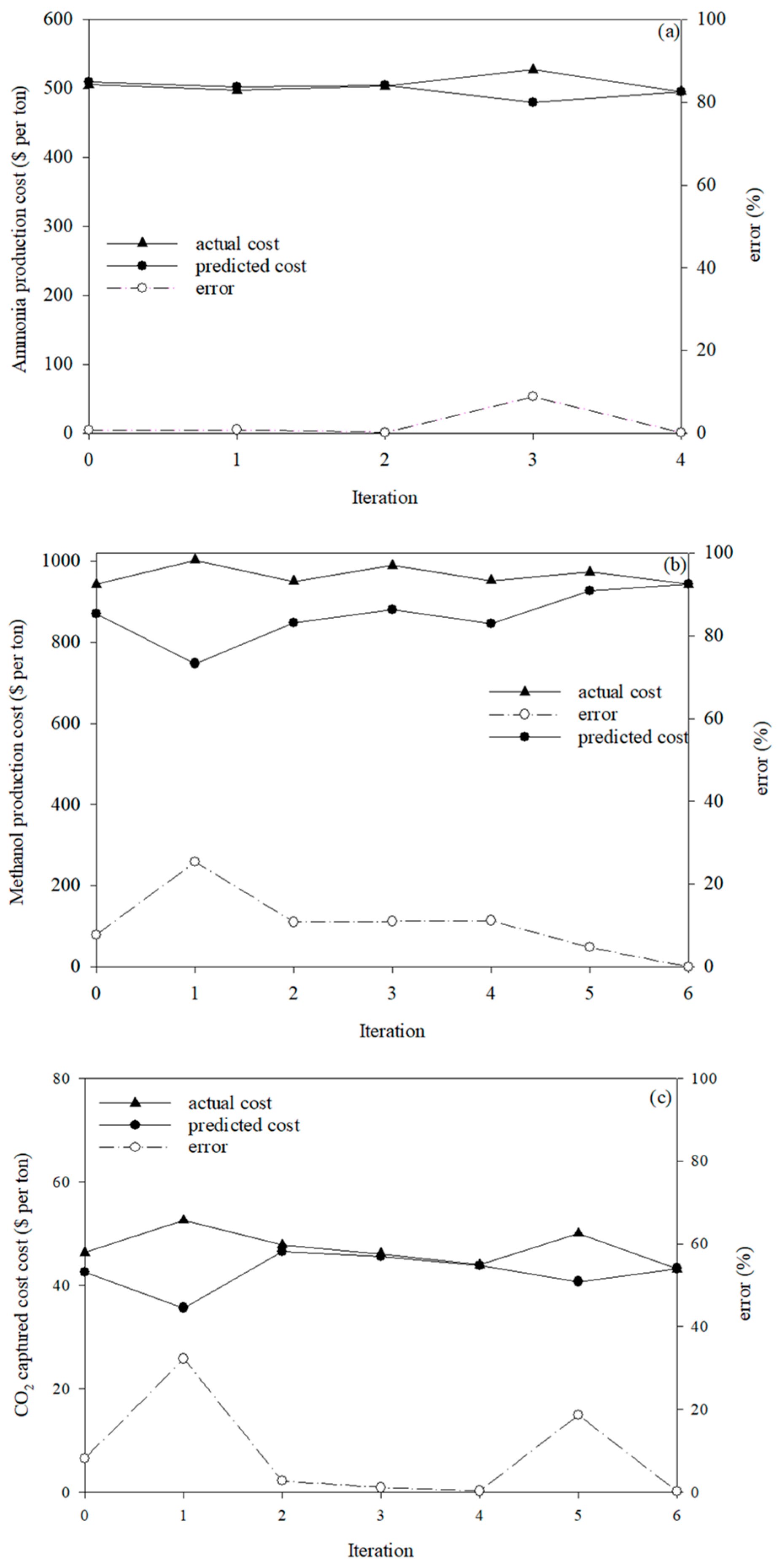
5.2. The Convergence of the Proposed Adaptive LSH Optimization Algorithm

Figure 10 illustrates the convergence of the proposed algorithm for all three case studies. In the figure, the triangle, black circle, and white circle symbols represent the actual cost (obtained from the process simulation), predicted cost (obtained from the optimization problem), and the percent error, respectively. The percent error between actual and predicted costs is depicted as a dashed line. The proposed algorithm terminates when the percent error of the optimal cost was less than one percent (1%).

For Case Studies I and III (Figure 10a,c), the outcomes exhibited a similar pattern, where the percent error decreased as more iterations were added. There were a few points where the percent error sharply rose before the algorithm converged. This was due to the fact that sample points for ANN training, testing, and validation were randomly chosen from the dataset, resulting in an insufficient number of data points before the algorithm converged. For Case Study II, as shown in Figure 10b, the percent error of the optimal solution decreased as the number of iterations (or sample points) increased until it eventually became less than one percent. In all three case studies, each of which featured a different number of independent parameters, the proposed method consistently converged to provide optimal results that met the necessary criteria. Details on the ANNs, including the weights and biases, for all three case studies, can be found in Supplementary Information S3.

Considering the scale of the case studies, the first case study, which included three studied factors, reached convergence after four iterations. Case Studies II and III, which had four and five studied factors, respectively, converged after six iterations. The results showed that the algorithm required more iterations to converge when dealing with higher-dimensional problems.

5.3. Comparison of Optimal Solutions between Proposed Sampling and Random Sampling

This section compares the outcomes of the proposed adaptive LHS optimization algorithm with those of random sampling to verify the results. Additionally, the number of sample points required to obtain the optimal solution is compared in this section. The number of sample points used in constructing the ANN model is crucial. Having a sufficient number of sample points to represent the relationship between independent and dependent variables allows the mathematical model to accurately depict the system, enabling the solver to find the true optimal solutions for the optimization problem.

Table 6. Comparison the results of proposed adaptive Latin hypercube sampling and random sampling.

Case Study I: Ammonia Production from Syngas
Sampling Techniques	Total number of sample points	R2	x1 (°C)	x2 (°C)	x3 (°C)	x4	x5	ypredicted ($\hat{y}$) (USD per ton)	yactual (y) (USD per ton)	% error
Random Sampling	100	0.9999	900	1400	160	N/A	N/A	496.73	495.87	0.17
Proposed algorithm
Replication 1	38	0.9928	900	1400	160	N/A	N/A	498.40	495.87	0.51
Replication 2	30	0.9995	900	1400	160	N/A	N/A	495.22	495.87	0.13
Replication 3	30	0.9987	900	1400	160	N/A	N/A	492.14	495.83	0.74
Case Study II: Methanol Production via Carbon Dioxide Hydrogenation
Sampling Techniques	Total number of sample points	R2	x1 (bar)	x2 (°C)	x3 (°C)	x4 (-)	x5	ypredicted ($\hat{y}$) (USD per ton)	yactual (y) (USD per ton)	% error
Random Sampling	100	1.0000	70	190	80	1	N/A	942.80	942.45	0.61
Proposed algorithm
Replication 1	46	1.0000	70	190	80	1	N/A	942.37	942.45	0.01
Replication 2	46	0.9993	70	190	80	1	N/A	943.85	942.45	0.15
Replication 3	40	0.9991	70	190	76	1	N/A	944.31	945.94	0.17
Case Study III: Carbon Dioxide Absorption by Methanol via Rectisol Process
Sampling Techniques	Total number of sample points	R2	x1 (°C)	x2 (bar)	x3 (-)	x4 (°C)	x5 (-)	ypredicted ($\hat{y}$) (USD per ton)	yactual (y) (USD per ton)	% error
Random Sampling	400	0.9998	−29.0	1.20	5	40	1	43.66	43.40	0.59
Proposed algorithm
Replication 1	53	0.9958	−20.0	1.20	5	40	1	45.74	45.47	0.60
Replication 2	50	0.9987	−20.0	1.27	5	40	1	45.91	45.67	0.51
Replication 3	53	0.9980	−26.7	1.28	5	40	1	43.25	43.19	0.14

provides a comparison of the optimal results obtained from random sampling and the proposed algorithm. Three replications of the proposed algorithm were conducted to ensure consistency. For Case Study I (ammonia production from syngas), the optimal operating conditions for all three variables obtained from the proposed algorithm matched those determined by random sampling. The optimal operating conditions were temperatures of 900 °C for the reformer, 1400 °C for the combuster, and 160 °C for the low-temperature conversion reactor, resulting in a minimum production cost of USD 495.87 per ton of generated ammonia, which was consistent with the results from random sampling. Notably, the proposed technique required only 38 sample points to find the optimal solution for this problem with three decision variables compared to the 100 sample points needed by random sampling.

The optimal operating conditions for Case Study II (methanol production from carbon dioxide hydrogenation) were determined using the proposed algorithm for three replications, and they matched those determined by random sampling, with the exception of the temperature of the steam entering the separator (x₃) in the third replication. In the third replication, the steam’s temperature entering the separator (x₃) is 76 °C, which was slightly different from the temperatures obtained in the other replications (80 °C). A slight decrease in the temperature of the stream entering the separator resulted in an increase in the methanol production cost. This change did not have a significant impact in terms of model prediction error. Furthermore, the third replication used only 40 sample points to represent the entire surface, while the other two replications used 46 sample points. This indicates that the model with 40 sample points found a local optimum. The optimal operating conditions for this case study were a pressure of 70 bar for the equilibrium reactor, a temperature of 190 °C for the reactor, a temperature of 80 °C for the steam entering a separator, and a recycling ratio of 1. The lowest cost to generate methanol was USD 942.45 per tonne of methanol. While random sampling required 100 sample points to find the optimal solution for this problem with four decision variables, the proposed adaptive LHS optimization approach only required 46 sample points.

For Case Study III (carbon dioxide absorption by methanol via the Rectisol process), the values of the optimal operating conditions were identical to those obtained from random sampling except for the value of the lean methanol temperature (x₁). The results for the lean methanol temperature (x₁) from three replications varied from −26.70 to −20.0 °C, which was slightly different from the values obtained from random sampling (−29.0 °C). The lowest CO₂ capture costs identified by the proposed algorithm for three replications ranged from USD 43.25 to USD 45.91 per ton of CO₂ capture, which is consistent with the lowest cost identified by random sampling (USD 43.40 per ton of CO₂ capture). The optimal operating parameters for this case study included a lean methanol temperature of −26.70 °C, a third-stage separator pressure of 1.28 bar, a stripper reflux ratio of 5, a stripper input temperature of 40 °C, and a distillation reflux ratio of 1. The minimum cost for CO₂ capture was USD 43.19 per tonne of CO₂. The proposed technique required only 53 sample points for this problem with five decision variables, while random sampling needed 400 sample points to achieve the same level of ANN model accuracy and obtain the optimal solutions.

Based on the results of the three different case studies, adaptive Latin hypercube sampling required fewer sample points than random sampling to accurately represent the entire surface using ANN models. The model accuracy and optimal conditions achieved using adaptive sampling were comparable to random sampling but required fewer sample points.

5.4. Recommendation for Future Work

To assess the performance of the current algorithm and establish its generalizability, it was compared to the work by [60], which introduced incremental Latin Hypercube Sampling (LHS) for ANN-based optimization. In [60], the sample size began at ten times the number of decision variables and increased iteratively by one-third of the current number of sample points, which was rounded up to the nearest tenth. In contrast, the present algorithm initiated with a sample size set at seven times the number of decision variables with three additional sample points added in each iteration. Both algorithms employed the same exit criteria (% error less than 1). The current algorithm required fewer additional sample points in each iteration and resulted in fewer sample points to obtain the optimal solution. However, it is important to note that the previous work applied their method to more complex problems involving six and seven decision variables. To comprehensively compare the performance of both methods, it is recommended to apply the current algorithm to optimization problems with higher dimensionality.

For future work, it is recommended to compare the performance of this adaptive LHS approach with other adaptive sampling techniques or advanced surrogate model techniques. Implementing Bayesian optimization to enhance the optimization method is suggested. Performance tests that incorporate various adaptive sampling criteria, such as distance, space-filling metrics, gradient information, and prediction uncertainty, can be applied to the algorithm. Furthermore, the results have demonstrated that as the number of samples increased, the solution converged to the true optimal solution. To enhance the performance of the algorithm, convergence guarantees can be further implemented. The application of the proposed algorithm should be extended to different fields of study, such as engineering design, materials discovery, etc. Additionally, it is essential to study the limitations of ANNs, particularly in terms of their consistency during the training process.

6. Conclusions

This paper proposes an adaptive Latin hypercube sampling method for simulation-based optimization problems. The algorithm uses the deviation of the output as a criterion for generating new sample points. After each iteration, three additional sample points are added to the existing dataset. The first additional sample point is the optimal solution from the previous optimization dataset, while the other two additional data points are selected from a grid area with the maximum deviation in output. Artificial neural networks (ANNs) were employed as the surrogate model for the optimization problem. The accuracy of the ANN model was assessed using the mean square error (MSE) and R-squared (R²) values. The criterion for determining the accuracy of the optimal solution was that the percent error should be less than one percent. The results demonstrate that the proposed algorithm is capable of obtaining optimal solutions that are similar to the random sampling approach but require fewer sample points.

One of the primary advantages of the developed algorithm is its versatility. While in this work, we exclusively applied adaptive sampling with ANNs, we envision broader applications across various surrogate models. The adaptability of the Latin hypercube sampling method makes it a valuable tool for optimizing complex systems where obtaining accurate models is crucial. Looking forward, we recommend a further exploration of adaptive Latin hypercube sampling in comparison to other adaptive sampling methods, particularly in the context of high-dimensional optimization problems. These future investigations will provide more insights into the algorithm’s scalability and efficiency.

References

1. Crombecq, K.; Laermans, E.; Dhaene, T. Efficient space-filling and non-collapsing sequential design strategies for simulation-based modeling. Eur. J. Oper. Res. 2011, 214, 683–696. [Google Scholar] [CrossRef]
2. Ahmadi, S.; Mesbah, M.; Igwegbe, C.A.; Ezeliora, C.D.; Osagie, C.; Khan, N.A.; Dotto, G.L.; Salari, M.; Dehghani, M.H. Sono electro-chemical synthesis of LaFeO3 nanoparticles for the removal of fluoride: Optimization and modeling using RSM, ANN and GA tools. J. Environ. Chem. Eng. 2021, 9, 105320. [Google Scholar] [CrossRef]
3. Bashir, M.J.; Amr, S.A.; Aziz, S.Q.; Ng, C.A.; Sethupathi, S. Wastewater treatment processes optimization using response surface methodology (RSM) compared with conventional methods: Review and comparative study. Middle-East J. Sci. Res. 2015, 23, 244–252. [Google Scholar]
4. Bezerra, M.A.; Santelli, R.E.; Oliveira, E.P.; Villar, L.S.; Escaleira, L.A. Response surface methodology (RSM) as a tool for optimization in analytical chemistry. Talanta 2008, 76, 965–977. [Google Scholar] [CrossRef]
5. Hoseiny, S.; Zare, Z.; Mirvakili, A.; Setoodeh, P.; Rahimpour, M. Simulation–based optimization of operating parameters for methanol synthesis process: Application of response surface methodology for statistical analysis. J. Nat. Gas Sci. Eng. 2016, 34, 439–448. [Google Scholar] [CrossRef]
6. Leonzio, G. Optimization through Response Surface Methodology of a Reactor Producing Methanol by the Hydrogenation of Carbon Dioxide. Processes 2017, 5, 62. [Google Scholar] [CrossRef]
7. Mohammad, N.K.; Ghaemi, A.; Tahvildari, K. Hydroxide modified activated alumina as an adsorbent for CO2 adsorption: Experimental and modeling. Int. J. Greenh. Gas Control 2019, 88, 24–37. [Google Scholar] [CrossRef]
8. Veljković, V.B.; Velickovic, A.V.; Avramović, J.M.; Stamenković, O.S. Modeling of biodiesel production: Performance comparison of Box–Behnken, face central composite and full factorial design. Chin. J. Chem. Eng. 2018, 27, 1690–1698. [Google Scholar] [CrossRef]
9. Simpson, T.W.; Poplinski, J.D.; Koch, P.N.; Allen, J.K. Metamodels for Computer-Based Engineering Design: Survey and Recommendations. Eng. Comput. 2001, 17, 129–150. [Google Scholar] [CrossRef]
10. Beers, W.C.M.v.; Kleijnen, J.P.C. Kriging interpolation in simulation: A survey. In Proceedings of the 2004 Winter Simulation Conference 2004, Washington, DC, USA, 5–8 December 2004. [Google Scholar]
11. Eason, J.; Cremaschi, S. Adaptive sequential sampling for surrogate model generation with artificial neural networks. Comput. Chem. Eng. 2014, 68, 220–232. [Google Scholar] [CrossRef]
12. Bliek, L. A Survey on Sustainable Surrogate-Based Optimisation. Sustainability 2022, 14, 3867. [Google Scholar] [CrossRef]
13. Panerati, J.; Schnellmann, M.A.; Patience, C.; Beltrame, G.; Patience, G.S. Experimental methods in chemical engineering: Artificial neural networks–ANNs. Can. J. Chem. Eng. 2019, 97, 2372–2382. [Google Scholar] [CrossRef]
14. Jin, Y.; Li, J.; Du, W.; Qian, F. Adaptive Sampling for Surrogate Modelling with Artificial Neural Network and Its Application in an Industrial Cracking Furnace. Can. J. Chem. Eng. 2016, 94, 262–272. [Google Scholar] [CrossRef]
15. Vaklieva-Bancheva, N.G.; Vladova, R.K.; Kirilova, E.G. Simulation of heat-integrated autothermal thermophilic aerobic digestion system operating under uncertainties through artificial neural network. Chem. Eng. Trans. 2019, 76, 325–330. [Google Scholar]
16. Hoseinian, F.S.; Rezai, B.; Kowsari, E.; Safari, M. A hybrid neural network/genetic algorithm to predict Zn(II) removal by ion flotation. Sep. Sci. Technol. 2020, 55, 1197–1206. [Google Scholar] [CrossRef]
17. Bahrami, S.; Ardejani, F.D.; Baafi, E. Application of artificial neural network coupled with genetic algorithm and simulated annealing to solve groundwater inflow problem to an advancing open pit mine. J. Hydrol. 2016, 536, 471–484. [Google Scholar] [CrossRef]
18. Mousavi, S.M.; Mostafavi, E.S.; Jiao, P. Next generation prediction model for daily solar radiation on horizontal surface using a hybrid neural network and simulated annealing method. Energy Convers. Manag. 2017, 153, 671–682. [Google Scholar] [CrossRef]
19. Zendehboudi, S.; Rezaei, N.; Lohi, A. Applications of hybrid models in chemical, petroleum, and energy systems: A systematic review. Appl. Energy 2018, 228, 2539–2566. [Google Scholar] [CrossRef]
20. Eslamimanesh, A.; Gharagheizi, F.; Mohammadi, A.H.; Richon, D. Artificial neural network modeling of solubility of supercritical carbon dioxide in 24 commonly used ionic liquids. Chem. Eng. Sci. 2011, 66, 3039–3044. [Google Scholar] [CrossRef]
21. Mohammadpoor, M.; Torabi, F. A new soft computing-based approach to predict oil production rate for vapour extraction (VAPEX) process in heavy oil reservoirs. Can. J. Chem. Eng. 2018, 96, 1273–1283. [Google Scholar] [CrossRef]
22. Bhutani, N.; Rangaiah, G.; Ray, A. First-principles, data-based, and hybrid modeling and optimization of an industrial hydrocracking unit. Ind. Eng. Chem. Res. 2006, 45, 7807–7816. [Google Scholar] [CrossRef]
23. Zorzetto, L.F.M.; Filho, R.M.; Wolf-Maciel, M. Processing modelling development through artificial neural networks and hybrid models. Comput. Chem. Eng. 2000, 24, 1355–1360. [Google Scholar] [CrossRef]
24. Tahkola, M.; Keranen, J.; Sedov, D.; Far, M.F.; Kortelainen, J. Surrogate Modeling of Electrical Machine Torque Using Artificial Neural Networks. IEEE Access 2020, 8, 220027–220045. [Google Scholar] [CrossRef]
25. Adeli, H. Neural Networks in Civil Engineering: 1989–2000. Comput.-Aided Civ. Infrastruct. Eng. 2001, 16, 126–142. [Google Scholar] [CrossRef]
26. Arora, S.; Shen, W.; Kapoor, A. Neural network based computational model for estimation of heat generation in LiFePO4 pouch cells of different nominal capacities. Comput. Chem. Eng. 2017, 101, 81–94. [Google Scholar] [CrossRef]
27. Himmelblau, D.M. Applications of artificial neural networks in chemical engineering. Korean J. Chem. Eng. 2000, 17, 373–392. [Google Scholar] [CrossRef]
28. Shahin, M.A.; Jaksa, M.B.; Maier, H.R. State of the art of artificial neural networks in geotechnical engineering. Electron. J. Geotech. Eng. 2008, 8, 1–26. [Google Scholar]
29. Nayak, R.; Jain, L.C.; Ting, B.K.H. Artificial Neural Networks in Biomedical Engineering: A Review. In Computational Mechanics–New Frontiers for the New Millennium; Valliappan, S., Khalili, N., Eds.; Elsevier: Oxford, UK, 2001; pp. 887–892. [Google Scholar]
30. Wang, C.; Luo, Z. A Review of the Optimal Design of Neural Networks Based on FPGA. Appl. Sci. 2022, 12, 771. [Google Scholar] [CrossRef]
31. Garud, S.S.; Karimi, I.A.; Kraft, M. Design of computer experiments: A review. Comput. Chem. Eng. 2017, 106, 71–95. [Google Scholar] [CrossRef]
32. Morshed, M.N.; Pervez, N.; Behary, N.; Bouazizi, N.; Guan, J.; Nierstrasz, V.A. Statistical Modeling and Optimization of Heterogeneous Fenton-like Removal of Organic Pollutant Using Fibrous Catalysts: A Full Factorial Design. Sci. Rep. 2020, 10, 16133. [Google Scholar] [CrossRef]
33. Villa Montoya, A.C.; Mazareli, R.C.d.S.; Delforno, T.P.; Centurion, V.B.; de Oliveira, V.M.; Silva, E.L.; Varesche, M.B.A. Optimization of key factors affecting hydrogen production from coffee waste using factorial design and metagenomic analysis of the microbial community. Int. J. Hydrogen Energy 2020, 45, 4205–4222. [Google Scholar] [CrossRef]
34. McKay, M.D.; Beckman, R.J.; Conover, W.J. A Comparison of Three Methods for Selecting Values of Input Variables in the Analysis of Output from a Computer Code. Technometrics 1979, 21, 239–245. [Google Scholar]
35. Sheikholeslami, R.; Razavi, S. Progressive Latin Hypercube Sampling: An Efficient Approach for Robust Sampling-Based Analysis of Environmental Models. Environ. Model. Softw. 2017, 93, 109–126. [Google Scholar] [CrossRef]
36. Grosso, A.; Jamali, A.R.M.J.U.; Locatelli, M. Finding Maximin Latin Hypercube Designs by Iterated Local Search heuristics. Eur. J. Oper. Res. 2009, 197, 541–547. [Google Scholar] [CrossRef]
37. Morris, M.D.; Mitchell, T.J. Exploratory designs for computational experiments. J. Stat. Plan. Inference 1995, 43, 381–402. [Google Scholar] [CrossRef]
38. Pholdee, N.; Bureerat, S. An efficient optimum Latin hypercube sampling technique based on sequencing optimisation using simulated annealing. Int. J. Syst. Sci. 2015, 46, 1780–1789. [Google Scholar] [CrossRef]
39. Park, J.-S. Optimal Latin-hypercube designs for computer experiments. J. Stat. Plan. Inference 1994, 39, 95–111. [Google Scholar] [CrossRef]
40. Ye, K.Q.; Li, W.; Sudjianto, A. Algorithmic construction of optimal symmetric Latin hypercube designs. J. Stat. Plan. Inference 2000, 90, 145–159. [Google Scholar] [CrossRef]
41. Fang, K.-T. Theory, Method and Applications of the Uniform Design. Int. J. Reliab. Qual. Saf. Eng. 2002, 9, 305–315. [Google Scholar] [CrossRef]
42. Bates, S.; Sienz, J.; Toropov, V. Formulation of the Optimal Latin Hypercube Design of Experiments Using a Permutation Genetic Algorithm. In Proceedings of the 45th AIAA/ASME/ASCE/AHS/ASC Structures, Structural Dynamics & Materials Conference, Palm Springs, CA, USA, 19–22 April 2004; American Institute of Aeronautics and Astronautics: Reston VA, USA, 2004. [Google Scholar]
43. Jin, R.; Chen, W.; Sudjianto, A. An efficient algorithm for constructing optimal design of computer experiments. J. Stat. Plan. Inference 2005, 134, 268–287. [Google Scholar] [CrossRef]
44. Van Dam, E.R.; Husslage, B.; Hertog, D.D.; Melissen, H. Maximin Latin Hypercube Designs in Two Dimensions. Oper. Res. 2007, 55, 158–169. [Google Scholar] [CrossRef]
45. Viana, F.A.C.; Venter, G.; Balabanov, V. An algorithm for fast optimal Latin hypercube design of experiments. Int. J. Numer. Methods Eng. 2010, 82, 135–156. [Google Scholar] [CrossRef]
46. Aziz, M.; Tayarani-N, M.-H. An adaptive memetic Particle Swarm Optimization algorithm for finding large-scale Latin hypercube designs. Eng. Appl. Artif. Intell. 2014, 36, 222–237. [Google Scholar] [CrossRef]
47. Chen, R.-B.; Hsieh, D.-N.; Hung, Y.; Wang, W. Optimizing Latin hypercube designs by particle swarm. Stat. Comput. 2013, 23, 663–676. [Google Scholar] [CrossRef]
48. Pan, G.; Ye, P.; Wang, P. A Novel Latin hypercube algorithm via translational propagation. Sci. World J. 2014, 2014, 163949. [Google Scholar] [CrossRef] [PubMed]
49. Husslage, B.G.M.; Rennen, G.; van Dam, E.R.; Hertog, D.D. Space-filling Latin hypercube designs for computer experiments. Optim. Eng. 2011, 12, 611–630. [Google Scholar] [CrossRef]
50. Wang, G.G. Adaptive Response Surface Method Using Inherited Latin Hypercube Design Points. J. Mech. Des. 2003, 125, 210–220. [Google Scholar] [CrossRef]
51. Chang, Y.; Sun, Z.; Sun, W.; Song, Y. A New Adaptive Response Surface Model for Reliability Analysis of 2.5D C/SiC Composite Turbine Blade. Appl. Compos. Mater. 2018, 25, 1075–1091. [Google Scholar] [CrossRef]
52. Roussouly, N.; Petitjean, F.; Salaun, M. A new adaptive response surface method for reliability analysis. Probabilistic Eng. Mech. 2013, 32, 103–115. [Google Scholar] [CrossRef]
53. Liu, Z.-z.; Li, W.; Yang, M. Two General Extension Algorithms of Latin Hypercube Sampling. Math. Probl. Eng. 2015, 2015, 450492. [Google Scholar] [CrossRef]
54. Liu, Z.; Yang, M.; Li, W. A Sequential Latin Hypercube Sampling Method for Metamodeling. In Theory, Methodology, Tools and Applications for Modeling and Simulation of Complex Systems; Springer: Singapore, 2016. [Google Scholar]
55. Metropolis, N.; Ulam, S. The Monte Carlo Method. J. Am. Stat. Assoc. 1949, 44, 335–341. [Google Scholar] [CrossRef] [PubMed]
56. Anawkar, S.; Panchwadkar, A. Comparison between Levenberg Marquart, Bayesian and scaled conjugate algorithm for prediction of cutting forces in face milling operation. AIP Conf. Proc. 2022, 2653, 030006. [Google Scholar]
57. Borisut, P.; Nuchitprasittichai, A. Process Configuration Studies of Methanol Production via Carbon Dioxide Hydrogenation: Process Simulation-Based Optimization Using Artificial Neural Networks. Energies 2020, 13, 6608. [Google Scholar] [CrossRef]
58. Janosovský, J.; Danko, M.; Labovský, J.; Jelemenský, L. Software approach to simulation-based hazard identification of complex industrial processes. Comput. Chem. Eng. 2019, 122, 66–79. [Google Scholar] [CrossRef]
59. Adams, T.A.; Salkuyeh, Y.K.; Nease, J. Chapter 6—Processes and simulations for solvent-based CO2 capture and syngas cleanup. In Reactor and Process Design in Sustainable Energy Technology; Shi, F., Ed.; Elsevier: Amsterdam, The Netherlands, 2014; pp. 163–231. [Google Scholar]
60. Nuchitprasittichai, A.; Cremaschi, S. An algorithm to determine sample sizes for optimization with artificial neural networks. AIChE J. 2013, 59, 805–812. [Google Scholar] [CrossRef]
Figure 1. Illustration of Latin hypercube sampling for N = 10 of (a) good filling design and (b) poor filling design.
Processes 11 03232 g001
Figure 2. Illustration of random sampling for (a) N = 10, (b) N = 100.
Processes 11 03232 g002
Figure 3. The schematic of feedforward neural networks.
Processes 11 03232 g003
Figure 4. Proposed adaptive Latin hypercube sampling for surrogate-based optimization.
Processes 11 03232 g004
Figure 5. Additional sample points generation using maximum deviation. (a) original Latin hypercube sampling and (b) adaptive Latin hypercube sampling.
Processes 11 03232 g005
Figure 6. Random sampling for optimization.
Processes 11 03232 g006
Figure 7. Process simulation of ammonia production from syngas.
Processes 11 03232 g007
Figure 8. Process simulation of methanol production via carbon dioxide hydrogenation.
Processes 11 03232 g008
Figure 9. Process simulation of CO2 captured via Rectisol process.
Processes 11 03232 g009
Figure 10. The convergence of the proposed algorithm for all three case studies: (a) ammonia production from syngas, (b) the production of methanol from carbon dioxide hydrogenation, (c) carbon dioxide absorption by methanol via Rectisol process.
Processes 11 03232 g010