Improving Accuracy and Interpretability of CNN-Based Fault Diagnosis through an Attention Mechanism

Abstract

This study aims to enhance the accuracy and interpretability of fault diagnosis. To address this objective, we present a novel attention-based CNN method that leverages image-like data generated from multivariate time series using a sliding window processing technique. By representing time series data in an image-like format, the spatiotemporal dependencies inherent in the raw data are effectively captured, which allows CNNs to extract more comprehensive fault features, consequently enhancing the accuracy of fault diagnosis. Moreover, the proposed method incorporates a form of prior knowledge concerning category-attribute correlations into CNNs through the utilization of an attention mechanism. Under the guidance of thisprior knowledge, the proposed method enables the extraction of accurate and predictive features. Importantly, these extracted features are anticipated to retain the interpretability of the prior knowledge. The effectiveness of the proposed method is verified on the Tennessee Eastman chemical process dataset. The results show that proposed method achieved a fault diagnosis accuracy of 98.46%, which is significantly higher than similar existing methods. Furthermore, the robustness of the proposed method is analyzed by sensitivity analysis on hyperparameters, and the interpretability is revealed by visually analyzing its feature extraction process.

1. Introduction

Fault diagnosis serves as a crucial technology to ensure the normal operation of industrial activities. Over recent years, there has been a surge in the popularity of data-driven fault diagnosis methods [1,2,3,4,5,6,7] due to the convenient and cost-effective collection of real-time time series data. Among these methods, those based on deep learning (DL) [2,4,5,6,7] have gained significant attention and achieved remarkable outcomes, primarily because of their superior feature extraction capabilities. DL architectures, such as deep belief networks (DBN) [8], recurrent neural networks (RNN) [9], and convolutional neural networks (CNN) [2,10], have been applied in fault diagnosis research. Notably, CNN has emerged as the most widely used DL architecture in fault diagnosis, owing to its ability to extract complex high-dimensional features.

Most of the existing DL-based methods focus on how to obtain higher fault diagnosis accuracy. They achieve this goal by increasing the number of network layers [7] or adopting a hybrid network structure [11,12]. However, these methods are prone to overfitting when the data are limited. In particular, data scarcity poses a significant challenge in the field of fault diagnosis. On one hand, collecting an adequate amount of fault data is often impractical due to limitations such as machines or systems not being allowed or able to operate in a fault state for an extended period. On the other hand, generating fault data through simulation is a costly endeavor. To this end, some additional tricks, such as residual connection [13], data augmentation [14], pre-training [2], and meta-transfer learning [15], have been used to achieve high accuracy in the case of data scarcity. For example, Yu et al. (2022) developed a six-layer residual neural network for fault diagnosis and showed that it effectively enhances the accuracy of fault diagnosis [13]. Li et al. (2020) used data augmentation technology to artificially create additional valid data, which helped the DL-based approach to be able to cope with complex fault diagnosis with limited data [14]. Feng et al. (2020) proposed a novel domain-knowledge-based deep-broad learning framework to address the data scarcity problem in fault diagnosis, where a CNN-based feature extractor was pre-trained with the use of bridge labels [2]. Li et al. (2023) developed an attention-based deep meta-transfer learning method that is able to cope with the few-shot fine-grained fault diagnosis problem [15].

In addition to accuracy, interpretability is another significant concern of fault diagnosis methods. The outcome of fault diagnosis carries immense significance, and any inaccuracies in the results can lead to substantial losses. Consequently, ensuring the reliability of fault diagnosis results typically necessitates interpretability in the fault diagnosis method. However, data-driven approaches, particularly DL, are often referred to as “black box” methods that inherently lack interpretability. As a result, applying these approaches to real-world fault diagnosis scenarios becomes challenging. In recent years, researchers have started to pay attention to this issue, and have proposed several solutions. The first one is to employ visualization techniques, such as neuron activation maximization [16] and class activation mapping (CAM) [17], to analyze the features learned by DL models [18]. These visualization techniques can help us clearly investigate what DL models have learned. The second one is to incorporate interpretable prior knowledge into DL models [19,20]. For instance, Yu and Liu (2020) introduced a knowledge-based DBN that successfully incorporated confidence and classification rules into the DBN, leading to enhanced model interpretability [19]. The third approach is to utilize attention mechanisms [18,21,22]. For instance, Li et al. (2019) applied the attention mechanism to understand and improve DL-based fault diagnosis of rolling bearing [18].

The existing studies on ways to improve fault diagnosis accuracy or interpretability are shown in

Table 1. Existing ways to improve fault diagnosis accuracy or interpretability.

Study	Accuracy	Interpretability
Jia et al. [7]	Through a deeper network	/
Huang et al. [11], Xu et al. [12]	Through a hybrid network	/
Li et al. [18]	/	Through visualization techniques
Yu and Liu [19], Xie et al. [20]	/	Through prior knowledge integration
Li et al. [18], Liao et al. [21], Peng et al. [22]	/	Through attention mechanisms

. It is demonstrated that enhancing the accuracy of DL-based fault diagnosis methods generally necessitates an increase in model complexity. This might involve augmenting network layers or employing hybrid network architectures, among other strategies. However, such enhancements may inadvertently compromise model interpretability, which runs counter to our ultimate objective. Conversely, when striving to enhance interpretability, it is essential to incorporate supplementary elements like attention mechanisms and the integration of prior knowledge. It is noteworthy that prior studies [18,21,22] have underscored the capacity of attention mechanisms to enhance fault diagnosis accuracy. Nevertheless, these studies failed to explore the potential benefits of prior knowledge integration. Consequently, this study aims to bridge this research gap by leveraging the attention mechanism to integrate prior knowledge, thereby concurrently enhancing both the accuracy and interpretability of fault diagnosis.

In this study, we focus on both the accuracy and interpretability of fault diagnosis. First, we used the sliding window method [11] to obtain the image-like data for constructing a CNN-based model. The obtained image-like data integrates the spatiotemporal dependence in the raw time series data so that the CNN is able to extract more abundant fault features, thereby improving the accuracy of fault diagnosis. Then, a kind of prior knowledge about the correlation between faults and attributes is formally defined based on the image-like data. Finally, the defined prior knowledge is integrated into the CNN based on an attention mechanism. In this way, accurate and predictive features can be extracted under the guidance of the defined prior knowledge. Moreover, the extracted features are expected to inherit the interpretability of the prior knowledge. In summary, the main contributions of this study lie in the definition of prior knowledge about category–attribute correlation and the integration of prior knowledge based on an attention mechanism.

The effectiveness and efficiency of the proposal were verified in the TE chemical process dataset [23]. The results show that the proposal significantly outperforms traditional data-driven, as well as recent DL-based, fault diagnosis methods in terms of accuracy. Moreover, the feature extraction process of the attention-based CNN model was analyzed by visualization techniques, which demonstrates its interpretability.

The rest of this paper is organized as follows. In Section 2, related works of CNN variants that are also able to fuse prior knowledge are presented. Section 3 introduces some basic knowledge about CNN and sliding window processes. Section 4 presents the proposed attention-based CNN method for fault diagnosis. In Section 5, the implementation of the proposed method to deal with the fault diagnosis of the TE chemical process is illustrated with analysis and discussion of results. Finally, conclusions and future work are provided in Section 6.

2. Related Works

To highlight the novelty of the proposed attention-based CNN, this section introduces related CNN variants that are also able to fuse prior knowledge, similar to the proposed one.

2.1. Region Proposals Convolutional Neural Networks

In the field of object detection, region proposals convolutional neural networks (R-CNNs) are a widely-used class of CNNs [24,25,26,27]. The core idea of R-CNNs is to combine region proposals generated by a particular region proposal method, such as selective search [28], with CNNs. The region proposals preliminarily locate the region of objects, which provides CNNs with informative data regions for feature extraction. As can be seen, the function of the region proposals is similar to that of the defined prior knowledge about the correlation between faults and attributes, which shows the consistency of core ideas between R-CNNs and the proposed method. Nevertheless, acquisition methods of the prior knowledge and the region proposals are completely different. Furthermore, the region proposals are directly used as the input of CNNs for feature extraction, while in this study the defined prior knowledge about the correlation between faults and attributes can be integrated into any layer of CNN, which enables deeper and more flexible integration of prior knowledge.

2.2. Mask-Based Convolutional Neural Networks

Mask-based convolutional neural networks (MCNNs) are a class of CNNs used to avoid background noise, and have been applied to person retrieval [29]. In MCNNs, a latent binary mapping of the raw data is first learned by a specific neural network, such as the fully convolutional network [29] or the U-net [30]. The learned latent binary mapping extracts regions of interest from the raw data that contain informative signals for subsequent tasks, which is similar to the prior knowledge defined in this study. After that, the so-called masked data obtained by the operation of element-wise product between the learned latent binary mapping and the raw data is directly used as the input of CNNs for feature extraction. Although both MCNNs and the proposed method achieve the location of informative region of the raw data, the former does not realize the coupling of the learned latent binary mapping with any layer of CNN.

2.3. Squeeze-and-Excitation Networks

Squeeze-and-excitation (SE) networks are developed by stacking a novel architectural unit, the SE block, which achieves excellent results on a variety of tasks such as face recognition [31] and image classification [32]. The SE block is used to selectively highlight informative channel-wise features by explicitly modeling interdependencies between channels of its intermediate features [33]. More specifically, two steps, namely squeeze and excitation, are involved in the calculation process of the SE block, where squeeze uses global average pooling to generate channel-wise statistics for exploiting channel dependencies and excitation adopts a simple gating mechanism with a sigmoid activation to make use of the information aggregated in the step of squeeze. The gating mechanism results in additional network parameters, thus adding computational cost. Conversely, the proposed method, which also has a flexible architectural unit for capturing informative data region, namely the attention module, is constructed without any parameters.

3. Basic Knowledge

This section presents basic knowledge needed for subsequent discussions, such as convolutional neural networks and sliding window processing.

3.1. Convolutional Neural Networks

CNNs were originally proposed by Krizhevsky et al. (2012) for image recognition [34]. Now, CNNs have become the cornerstone of DL. A CNN generally consists of a feature extractor and a classifier, where the feature extractor is composed of certain stacked convolutional and pooling layers. In a convolutional layer, the input undergoes convolution with a trainable kernel, followed by the operation of an activation function to produce the output. The input or output is a set of feature maps denoted as $X=[X_1,\dots ,X_i,\dots ,X_n]$, where $X_i\in R^{w\times h}(i=1,\dots ,n)$ is called a feature map with size $(w,h)$. Assuming that $X^{in}$ denotes the input with $m$ feature maps, $X^{out}$ denotes the output with $n$ feature maps, and $K=[K_1,\dots ,K_j,\dots ,K_n]$ denotes the convolutional kernel that is composed of $n$ filters $K_j\in R^{k\times l}(j=1,\dots ,n)$ with size $(k,l)$, the operation of a convolutional layer is shown in the following formula:

$$X_j^{out}=f\left(\sum _{i=1}^m{X}_i^{in}\ast K_j+b_j\right)\left(j=1,\dots ,n\right),$$

(1)

where $b_j$ denotes the bias corresponding to the $j$th filter $K_j$, $f(\bullet )$ denotes a nonlinear activation function (e.g., the rectified linear unit), and $\ast$ denotes the convolutional operation. After a convolutional layer, a pooling layer produces a down sampled version of the obtained feature maps.

The classifier seeks to classify samples into corresponding categories according to the feature maps extracted by the feature extractor. The classifier generally consists of some stacked fully connected (FC) layers and a final softmax operation. The feature maps are compressed into a feature vector as the inputs of the first FC layer. A softmax operation is applied to the output of the last FC layer to obtain the category probability vector.

3.2. Sliding Window Processing

Fault diagnosis typically utilizes raw data in the form of time series, which can be categorized into two types: univariate time series (UTS) and multivariate time series (MTS) [35]. A UTS $S_T=[s_1,\dots ,s_t,\dots ,s_T]$ is a vector with elements in chronological order, where $T$ denotes the length. A K-dimensional MTS $S_T^K=[S_T\left(c_1\right),\dots ,S_T\left(c_k\right),\dots ,S_T\left(c_K\right)]$ is a matrix, where $S_T\left(c_k\right)$ denotes an UTS associated with the attribute $c_k\in C=\left\{c_k\right|k=1,\dots ,K\}$. In this study, the raw data used for fault diagnosis are denoted as a K-dimensional MTS $S_T^K$. However, $S_T^K$ generally cannot be directly used as the input of DL-based fault diagnosis method due to the fact that $T$ is usually very large and the formalism of $S_T^K$ cannot meet the input requirements of the developed fault diagnosis method. To this end, a certain data transformation method is required to obtain data samples that meet the input requirements of the developed fault diagnosis method from $S_T^K$.

In this study, we use the sliding window processing (SWP) [11] to obtain samples from $S_T^K$. Since we are constructing a fault diagnosis model using CNNs, the input data format should be image-like; that is, the samples obtained from $S_T^K$ by SWP should be image-like. More specifically, the image-like samples are obtained by simultaneously performing SWP on the raw time series $S_T^K$ and $Y_T^M$, where $Y_T^M$ denotes a series of one-hot vectors used to represent the category at each moment of $S_T^K$. For example, given a system has three fault states (Faults 1, 2, and 3) and one normal state. If the system state at a certain moment is Fault 1, then a one-hot vector [0, 1, 0, 0] is used to represent such a system state. In this way, within consecutive moments, we can obtain a series of one-hot vectors. Arranging these one-hot vectors in chronological order, we then obtain $Y_T^M$ that is also an MTS, as we can see, where M denotes the total number of system states and T denotes the length of the consecutive moments. A detailed description to the process of SWP for $S_T^K$ and $Y_T^M$ is shown in Figure 1. As can be seen in Figure 1, SWP has a sliding window that is a rectangular frame used to obtain sub-series from $S_T^K$ and $Y_T^M$. Sub-series are continuously obtained by moving the sliding window. Assuming the width of the sliding window is an integer $d(0<d\le T)$ and the step size of the movement of the sliding window is an integer $\lambda (0<\lambda \le T-d)$, SWP is represented as $W(d,\lambda )$. Let the $i$th sub-series obtained by $W(d,\lambda )$ be ${\left(S_d^K\right)}_i$ for $S_T^K$, and ${\left(Y_d^M\right)}_i$ for $Y_T^M$. The last element of ${\left(Y_d^M\right)}_i$ is denoted as ${\left(y_m\right)}_i(m=1,\dots ,M)$, that is considered as the category of ${\left(S_d^K\right)}_i$. Then, the tuple $<{\left(S_d^K\right)}_i,{\left(y_m\right)}_i>$ can be considered as the sample obtained by the $i$th movement of the sliding window. In this way, an image-like data set $D=\{<{\left(S_d^K\right)}_i,Y_i>|i=1,\dots ,N\}$ can be obtained by constantly moving the sliding window, where N denotes the number of the obtained samples.

To explain the above sliding window processing more clearly, let’s give an example below. Suppose a system has two fault states and one normal state. We detect the operating state of the system by observing four system properties. To this end, we collect the observed system attribute data in five consecutive moments, namely $S_5^4$, as follows:

$$S_5^4=\left(\begin{array}{cccc}0.50& 0.10& 0.91& 0.40\\ 0.49& 0.11& 0.90& 0.40\\ 0.48& 0.09& 0.91& 0.41\\ 0.51& 0.11& 0.92& 0.39\\ 0.60& 0.01& 0.10& 0.38\end{array}\right)$$

Similarly, we record the system states $Y_5^3$ in the manner of one-hot vectors,

$$Y_5^3=\left(\begin{array}{ccc}1& 0& 0\\ 1& 0& 0\\ 1& 0& 0\\ 1& 0& 0\\ 0& 1& 0\end{array}\right)$$

With the use of a SWP $W(3,1)$, at the first move of the sliding window we obtain the following image-like data and their corresponding label:

$${\left(S_3^4\right)}_1=\left(\begin{array}{cccc}0.50& 0.10& 0.91& 0.40\\ 0.49& 0.11& 0.90& 0.40\\ 0.48& 0.09& 0.91& 0.41\end{array}\right),{\left(S_3^3\right)}_1=\left(\begin{array}{ccc}1& 0& 0\end{array}\right)$$

At the second move, the following results can be obtained:

$${\left(S_3^4\right)}_2=\left(\begin{array}{cccc}0.49& 0.11& 0.90& 0.40\\ 0.48& 0.09& 0.91& 0.41\\ 0.51& 0.11& 0.92& 0.39\end{array}\right),{\left(S_3^3\right)}_2=\left(\begin{array}{ccc}1& 0& 0\end{array}\right)$$

At the last move, the results come as:

$${\left(S_3^4\right)}_3=\left(\begin{array}{cccc}0.48& 0.09& 0.91& 0.41\\ 0.51& 0.11& 0.92& 0.39\\ 0.60& 0.01& 0.10& 0.38\end{array}\right),{\left(S_3^3\right)}_3=\left(\begin{array}{ccc}0& 1& 0\end{array}\right)$$

4. Attention-Based CNN for Fault Diagnosis

It is a fact that different attributes in MTS contribute differently to fault diagnosis. Although a classic CNN may be able to learn such correlation between attributes and fault categories, if such information can be given to CNNs in advance, the informative data regions will be located by the feature extractor, which enables the network to learn useful fault features more accurately and efficiently.

Attention mechanisms are a class of methods that enable the feature extractor of a CNN to selectively focus on specific regions of the data [36]. In this study, the attention mechanism [37] is used to assist the feature extractor in focusing on the data regions that have a large correlation with the faults. Firstly, the correlation between the data regions and faults is obtained from prior knowledge about category–attribute correlation that is defined based on the Pearson Correlation Coefficient (PCC). Then, the defined prior knowledge is integrated into the feature extractor of CNNs based on an attention mechanism. In this way, this attention-based CNN can pay attention to the correlation between data regions and faults when extracting features.

4.1. Prior Knowledge about Category-Attribute Correlation

4.1.1. Pearson Correlation Coefficient

PCC is commonly used to characterize the degree of linear correlation between two sequences $X=[x_1,\dots x_n]$ and $Y=[y_1,\dots y_n]$, which is often expressed as $r(X,Y)$ [38]. The following is its measurement method:

$$\overline{X}=\frac{1}{n}\sum _{i=1}^n{x}_i,$$

(2)

$$\overline{Y}=\frac{1}{n}\sum _{i=1}^n{y}_i,$$

(3)

and

$$r\left(X,Y\right)=\frac{\sum _{i=1}^n\left(x_i-\overline{X}\right)\left(y_i-\overline{Y}\right)}{\sqrt{\sum _{i=1}^n{\left(x_i-\overline{X}\right)}^2}\sqrt{\sum _{i=1}^n{\left(y_i-\overline{Y}\right)}^2}}.$$

(4)

One can see that $-1\le r\left(X,Y\right)\le 1$. When $r\left(X,Y\right)<(>)0$, it means that there is a negative (positive) correlation between $X$ and $Y$. When $r\left(X,Y\right)=0$, it means that there is absolutely no correlation between $X$ and $Y$. The size of $\left|r\left(X,Y\right)\right|$ represents the magnitude of the correlation between $X$ and $Y$. For more details, please see a previous study [39] that gave an explanation between PCC and correlation.

4.1.2. Category-Attribute Correlation Matrix

Based on the definition of PCC, we deduce the definition of prior knowledge about category-attribute correlation.

Definition 1:

Correlation between categories and attributes. Suppose that the fault type implicit in the raw time series $S_T^K$ is denoted as $f_m\in F=\left\{f_m\right|m=1,\dots ,M\}$, where $f_1$ denotes the normal category and $f_{\mu }(\mu =2,\dots ,M)$ denote the fault categories. Let’s use $Y_T\left(f_m\right)=\left[y_1,\dots ,y_t,\dots ,y_T\right](y_t\in \{1,m\left\}\right)$ to denote the corresponding category UTS associated with $S_T^K$. In other words, the fault category of $S_T^K$ at each moment is either $f_1$ or $f_m$. The PCC $r_{mk}=r\left(S_T\right(c_k),Y_T(f_m\left)\right)$ is used to represent the correlation between $f_m$ and $c_k$, where $S_T\left(c_k\right)\left(k=1,\dots ,K\right)$ is the $k$th column of $S_T^K$ that represents the UTS related to $c_k$.

Definition 2:

Category-attribute correlation matrix. The category-attribute correlation matrix is defined as $R={\left(r_{mk}\right)}_{M\times K}$, where $r_{mk}$ is the correlation between $f_m$ and $c_k$.

The category–attribute correlation matrix $R$, obtained from historical data or experience, is a kind of prior knowledge which accurately reflects the linear correlation between categories and attributes. If CNNs can use this prior knowledge in the process of feature extraction, they can accurately locate the informative data regions, thereby accurately extracting fault features. In what follows, the process that integrates $R$ into CNNs based on an attention mechanism is introduced in detail.

4.2. Integrating Prior Knowledge into CNNs Based on Attention Mechanism

The process of integrating prior knowledge into CNNs is shown in Figure 2.

Step 1: Defining a PCC threshold $r(0<r<1)$. The purpose of defining $r$ is to filter out the attributes that are not basically related to the category, while those are related to the category will be retained.

Note 1: To prevent loss of information, an attribute should be considered as long as it has a little correlation with the fault category, and thus the value of $r$ should be the one that is able to distinguish the correlations “None” and “Low”. According to the study [39], the value of $r$ should be set around 0.09. To retain useful information as much as possible, in this study we set r to 0.07, which is slightly smaller than 0.09. Furthermore, in Section 5.3.5, we present the analysis of impact of the setting of r on the results of the proposed method.

Step 2: Calculating the category–attribute attention matrix $A\left(r\right)={\left(a_{mk}\right)}_{M\times K}$. $A\left(r\right)$ reflects the attention relationship between categories and attributes. Its calculation method is as follows:

$$a_{mk}=\left\{\begin{array}{c}1if\left|r_{mk}\right|\ge r\\ 0if\left|r_{mk}\right|<r\end{array}\right..$$

(5)

Step 3: Calculating the attention matrix ${\left(A_d^K\right)}_i$ related to a sample $<{\left(S_d^K\right)}_i,{\left(y_m\right)}_i>$. ${\left(A_d^K\right)}_i$ reflects which data regions of ${\left(S_d^K\right)}_i$ need attention. The specific method to calculate ${\left(A_d^K\right)}_i$ is shown in Figure 3.

Step 4: Compressing the feature maps $X$ output from CNNs. The channel-wise average pooling operation and channel-wise max pooling operation are applied to $X$ to obtain the compressed feature maps ${\tilde{X}}_1$ and ${\tilde{X}}_2$, respectively.

$${\tilde{X}}_1^{kl}=s\left(\frac{1}{n}\sum _{i=1}^n{X}_i^{kl}\right),k=1,\dots ,w;l=1,\dots ,h,$$

(6)

and

$${\tilde{X}}_2^{kl}=s\left(\underset{i\in \left\{1,\dots ,n\right\}}{\mathit{max}}{X}_i^{kl}\right),k=1,\dots ,w;l=1,\dots ,h,$$

(7)

where $s\left(x\right)=\frac{1}{1+e^{-x}}$ is used to map $x$ to interval (0, 1).

Step 5: Fusing ${\left(A_d^K\right)}_i$, ${\tilde{X}}_1$ and ${\tilde{X}}_2$. ${\left(A_d^K\right)}_i$ implies the attention information of the sample, while ${\tilde{X}}_1$ and ${\tilde{X}}_2$ imply the hidden features extracted by CNNs. By fusing ${\left(A_d^K\right)}_i$, ${\tilde{X}}_1$, and ${\tilde{X}}_2$, the attention information is integrated into the feature extraction process of CNNs. Specifically, we use matrix addition for this fusion.

$$Y={\tilde{X}}_1+{\tilde{X}}_2+{\left(A_d^K\right)}_i,$$

(8)

where $Y\in R^{w\times h}$ is a matrix whose element reflects the degree of correlation between the data region of $X$ and the category.

Step 6: Calculating the weight matrix $W$. $W$ can be obtained by performing softmax operation on all elements of $Y$:

$$W_{ij}=\frac{e^{Y_{ij}}}{\sum _{i=1}^w\sum _{j=1}^h{e}^{Y_{ij}}}.$$

(9)

Step 7: Calculating the output feature maps $\widehat{X}$. Applying $W$ to $X$ can obtain the output feature maps $\widehat{X}=[{\widehat{X}}_1,\dots ,{\widehat{X}}_i,\dots ,{\widehat{X}}_n]$, which achieves the purpose of integrating prior knowledge into CNNs,

$${\widehat{X}}_i=X_i\times W,i=1,\dots ,n,$$

(10)

where $\times$ denotes the element-wise multiplication of matrix.

The attention mechanism can be employed at each layer of the feature extractor, allowing for its continuous application. By repeatedly applying the attention mechanism to the layers of the feature extractor, it becomes increasingly adept at focusing on prior knowledge, enhancing its effectiveness. Besides, we can see that the attention mechanism is parameter-free since the acquisition of the weight matrix does not require a learning process, but relies entirely on the fusion of prior knowledge and extracted features.

5. Case Study in Tennessee Eastman Chemical Process Benchmark

The TE chemical process data set has been used to test the proposed fault diagnosis method. A detailed introduction to the TE chemical data set can be seen in https://github.com/camaramm/tennessee-eastman-profBraatz. The models were written in Python 3.7 with the help of a DL library called Pytorch. The models were trained and tested on a PC with 64-bit macOS 10.15.7 operation system, 2.2-GHz Quad-core Intel Core i7 processor, and 16-GB RAM.

5.1. Tennessee EASTMAN Chemical Process Benchmark

The TE chemical process serves as a simulation process that closely mimics the actual flow of a chemical company. It has gained significant recognition as a benchmark for research in data-driven fault diagnosis [23]. In the TE chemical process, a total of 41 measured variables and 11 manipulated variables are involved. For the purpose of this study, a fault diagnosis model is constructed using a selection of 52 variables. The TE chemical process encompasses 21 predefined types of faults along with a normal state. To facilitate model training and testing, separate training and test sets are created for each fault type and the normal state. The sampling frequency for data collection is set at 3 min per sample. Each training set consists of 500 continuous samples, equivalent to 25 h of data, while each test set comprises 960 continuous samples, equivalent to 48 h of data. It is noteworthy that the initial 20 samples of each training set and the first 160 samples of each test set are obtained from the normal state of the TE chemical process. For additional information regarding the TE chemical process, refer to [40].

Note 2: In the original training sets for each type of fault, only 480 samples are collected and the first 20 normal samples are not collected. In this study, in order to ensure the consistency between the training sets and the test sets, we supplement the first 20 samples in the training set for normal state to the training sets for each type of fault.

5.2. Experiments

5.2.1. SWP for the TE Chemical Process Data Sets

As mentioned in Section 5.1, a total of 52 variables were selected to construct a fault diagnosis model. The data collected from these variables have different dimensions, and thus a commonly used data normalization method, referred to as z-score, was used to normalize data collected from different variables before the SWP operation on the TE chemical process data sets.

Once the z-score completed, the SWP $W\left(12,1\right)(d=12,\lambda =1)$ was used to obtain the inputs of the attention-based CNN from the TE chemical process data sets. $W\left(12,1\right)$ is performed on each original training set and test set that can be viewed as MTS. The number of the image-like samples obtained from each training set is 488, and it is 948 for each test set. There is a total of 22 training sets and 22 test sets. Therefore, the total number of image-like samples for training and testing is $22\times 488=\mathrm{10,736}$ and $22\times 948=\mathrm{20,856}$, respectively. The result of $W\left(12,1\right)$ for each original training set and test set is shown in

Table 2. The result of $W\left(12,1\right)$ for each training set and test set.

Categories	Data Set	Length of Time Series	$\mathbf{The}\mathbf{Number}\mathbf{of}\mathbf{Samples}\mathbf{Obtained}\mathbf{by}\mathit{W}\left(12,1\right)$ (Normal/Fault Category)
Normal	Training set	500	488 (488/0)
	Test set	960	948 (948/0)
Faults 1–21	Training set	500	488 (9/479)
	Test set	960	948 (49/899)

.

Note 3: The impact of the setting of d on the results will be discussed in detail in Section 5.3.4. The setting of λ affects the number of samples obtained by SWP. The larger the setting of λ, the smaller the number of samples obtained. In this study we are expected to obtain as many samples as possible, so we set λ to its minimum value of 1.

One can find from Table 2 that some samples obtained from the original training set and the test set for each fault category are labeled as normal category. In this case, the number of samples with normal category is greater than the number of samples with fault category, which is called category (class) imbalance [41]. Actually, one can avoid category imbalance by increasing $d$ if it will affect the classification results.

5.2.2. Model Training

For the fault diagnosis of the TE chemical process, an attention-based CNN model was constructed with detailed model architecture, shown in

Table 3. The architecture of the attention-based CNN model.

	Layer	Input Feature Maps Size	Output Feature Maps Size	Kernel Size/Stride/Padding
Feature extractor	Conv-1 *	$1\times 12\times 52$	$3\times d\times 52$	$7\times 7/1/3$
	MaxPool-1	$3\times 12\times 52$	$3\times d\times 52$	$7\times 7/1/3$
	Conv-2 *	$3\times 12\times 52$	$5\times d\times 52$	$3\times 3/1/1$
	MaxPool-2	$5\times 12\times 52$	$5\times d\times 52$	$3\times 3/1/1$
	Atten-1	$5\times 12\times 52/12\times 52$	$5\times d\times 52$	-
	Conv-3 *	$5\times 12\times 52$	$10\times d\times 52$	$3\times 3/1/1$
	MaxPool-3	$10\times 12\times 52$	$10\times d\times 52$	$3\times 3/1/1$
	Atten-2	$10\times 12\times 52/12\times 52$	$10\times d\times 52$	-
	Conv-4 *	$10\times 12\times 52$	$1\times d\times 52$	$3\times 3/1/1$
	MaxPool-4	$1\times 12\times 52$	$1\times d\times 52$	$3\times 3/1/1$
Classifier	FC-1 #	$625$	$22$	-
	Softmax	22	22	-

.

In Table 3, the convolutional layer marked with * means that the batch normalization (BN) method proposed in [42] was used to speed up the network training; the FC layer marked with # means that the dropout method proposed in [43] was used to prevent overfitting, where the probability of discarding neurons is set to $p=0.75$.

The constructed attention-based CNN model was trained in 100 epochs using Adam’s algorithm [44]. The learning rate was set to 0.0001 and the number of batch samples was set to 100. The mean squared error (MSE) loss was used as the optimization objective function for model training.

5.3. Results Analysis

5.3.1. Evaluation Indicators

After the model is trained on the training set, it can be evaluated on the test set. Indicators commonly used for evaluating fault diagnosis model are fault diagnosis rate (FDR) and false positive rate (FPR). Given a category $i$, ${FDR}_i$ represents the proportion of the number of samples correctly predicted to category $i$ to the number of samples with category $i$, and ${FPR}_i$ represents the proportion of the number of samples wrongly predicted to category $i$ to the number of samples without category $i$. They are calculated as

$${FDR}_i=\frac{{TP}_i}{{TP}_i+{TN}_i},$$

(11)

and

$${FPR}_i=\frac{{FN}_i}{{FN}_i+{FP}_i}.$$

(12)

The meaning of related symbols in Formulas (11) and (12) can be seen in

Table 4. Statistics used to evaluate the classification performance of category $i$.

	$\mathbf{Number}\mathbf{of}\mathbf{Samples}\mathbf{Predicted}\mathbf{to}\mathbf{Category}\mathit{i}$	$\mathbf{Number}\mathbf{of}\mathbf{Samples}\mathbf{Not}\mathbf{Predicted}\mathbf{to}\mathbf{Category}\mathit{i}$
Number of samples with category $i$	${TP}_i$	${TN}_i$
Number of samples without category $i$	${FP}_i$	${FN}_i$

.

Furthermore, the average FDR $\overline{FDR}$ and the average FPR $\overline{FPR}$ were used to evaluate the overall classification performance. Suppose there are a total of $M$ categories that need to be classified, then

$$\overline{FDR}=\frac{\sum _{i=1}^M{TP}_i}{\sum _{i=1}^M{TP}_i+{TN}_i},$$

(13)

and

$$\overline{FPR}=\frac{\sum _{i=1}^M{FN}_i}{\sum _{i=1}^M{FN}_i+{FP}_i}=1-\overline{FDR}.$$

(14)

5.3.2. Evaluation Result and Performance Comparison

Table 5 presents the specific FDR and FPR values for the proposed method, as well as representative methods proposed in previous research. The findings demonstrate that the proposal not only exhibits notable improvements in FDR and FPR performance across general fault categories, but also demonstrates accurate classification in challenging categories (such as fault 3, fault 9, and fault 15) where previous research struggled. These results indicate that the proposal significantly outperforms other data-driven fault diagnosis methods.

5.3.3. Analysis of Model Interpretability

Previous studies have predominantly utilized visualization techniques [45] and sensitivity analysis methods [46] to explore the interpretability of DL models. In this study, we employed visualization techniques to validate the interpretability of the proposed fault diagnosis method. To achieve this, we first utilized the trained attention-based CNN model to predict two different samples, denoted as ${\left(S_d^K\right)}_i$ and ${\left(S_d^K\right)}_j$, from the test set. Subsequently, we obtained the three-dimensional feature maps generated by the MaxPool-1 (M1), MaxPool-2 (M2), Atten-1 (A1), MaxPool-3 (M3), Atten-2 (A2), and MaxPool-4 (M4) layers. These three-dimensional feature maps were further transformed into two-dimensional feature maps through channel-wise average pooling, as per Equation (6). To facilitate visualization, the elements of the two-dimensional feature maps were mapped to the range of [0, 1] using min–max normalization. Finally, the variation in color was employed to represent the magnitude of the elements in the two-dimensional feature maps, resulting in the generation of Figure 4 and Figure 5.

Table 5. Performance comparison with other data-driven fault diagnosis methods.

Categories	FDR (%)					FPR (%)
	The Proposal	DL [47]	EDBN-2 [48]	MPLS [23]	PCA [49]	The Proposal	EDBN-2 [48]
Normal	96.85	-	90.80	-	86.25	1.60	3.34
Fault 1	99.76	100.00	100.00	100.00	96.56	0.00	0.00
Fault 2	99.76	99.75	100.00	98.88	96.88	0.00	0.08
Fault 3	93.08	-	-	18.75	-	4.60	-
Fault 4	100.00	100.00	100.00	100.00	96.88	0.00	0.01
Fault 5	99.75	98.88	100.00	100.00	96.88	0.40	0.00
Fault 6	100.00	100.00	100.00	100.00	99.48	0.00	0.00
Fault 7	100.00	100.00	100.00	100.00	99.27	0.00	0.00
Fault 8	98.23	97.88	98.29	98.63	94.90	0.20	0.22
Fault 9	95.24	-	-	12.13	-	0.30	-
Fault 10	98.79	99.25	80.81	91.13	87.81	0.14	0.67
Fault 11	99.77	89.25	99.74	83.25	77.81	0.00	0.00
Fault 12	99.78	99.75	100.00	99.88	97.81	0.30	0.00
Fault 13	100.00	99.75	91.98	95.50	79.17	0.00	0.00
Fault 14	99.09	95.13	100.00	100.00	98.23	0.20	0.00
Fault 15	92.33	-	-	23.25	-	7.20	-
Fault 16	97.97	99.50	75.56	94.28	79.90	0.12	0.67
Fault 17	100.00	99.75	100.00	97.13	86.46	0.00	0.00
Fault 18	100.00	99.50	93.43	91.25	72.81	0.00	0.00
Fault 19	98.30	96.75	95.53	94.25	91.56	0.40	0.27
Fault 20	98.80	99.38	93.17	91.50	88.54	0.60	0.00
Fault 21	98.60	-	83.44	72.75	95.00	1.80	1.17
Average	98.46	-	94.31	-	-	1.54	5.69

Table 5. Performance comparison with other data-driven fault diagnosis methods.

Categories	FDR (%)					FPR (%)
	The Proposal	DL [47]	EDBN-2 [48]	MPLS [23]	PCA [49]	The Proposal	EDBN-2 [48]
Normal	96.85	-	90.80	-	86.25	1.60	3.34
Fault 1	99.76	100.00	100.00	100.00	96.56	0.00	0.00
Fault 2	99.76	99.75	100.00	98.88	96.88	0.00	0.08
Fault 3	93.08	-	-	18.75	-	4.60	-
Fault 4	100.00	100.00	100.00	100.00	96.88	0.00	0.01
Fault 5	99.75	98.88	100.00	100.00	96.88	0.40	0.00
Fault 6	100.00	100.00	100.00	100.00	99.48	0.00	0.00
Fault 7	100.00	100.00	100.00	100.00	99.27	0.00	0.00
Fault 8	98.23	97.88	98.29	98.63	94.90	0.20	0.22
Fault 9	95.24	-	-	12.13	-	0.30	-
Fault 10	98.79	99.25	80.81	91.13	87.81	0.14	0.67
Fault 11	99.77	89.25	99.74	83.25	77.81	0.00	0.00
Fault 12	99.78	99.75	100.00	99.88	97.81	0.30	0.00
Fault 13	100.00	99.75	91.98	95.50	79.17	0.00	0.00
Fault 14	99.09	95.13	100.00	100.00	98.23	0.20	0.00
Fault 15	92.33	-	-	23.25	-	7.20	-
Fault 16	97.97	99.50	75.56	94.28	79.90	0.12	0.67
Fault 17	100.00	99.75	100.00	97.13	86.46	0.00	0.00
Fault 18	100.00	99.50	93.43	91.25	72.81	0.00	0.00
Fault 19	98.30	96.75	95.53	94.25	91.56	0.40	0.27
Fault 20	98.80	99.38	93.17	91.50	88.54	0.60	0.00
Fault 21	98.60	-	83.44	72.75	95.00	1.80	1.17
Average	98.46	-	94.31	-	-	1.54	5.69

From Figure 4, one can summarize the following findings:

• The raw data of ${\left(S_d^K\right)}_i$ and ${\left(S_d^K\right)}_j$ are indistinguishable, and the model cannot produce distinguishable features on the outputs of M1 after the raw data is processed by a convolutional layer and a pooling layer.
• From M1 to M2, some distinguishable striped features began to appear, as indicated by the red arrow. However, it can be seen that the striped features in the M2 outputs of ${\left(S_d^K\right)}_i$ and ${\left(S_d^K\right)}_j$ show some differences, which implies that the extracted features are biased. Specifically, taking the area framed by dotted rectangle in the outputs of M2 as an example, that of ${\left(S_d^K\right)}_i$ shows light yellow, while that of ${\left(S_d^K\right)}_j$ shows light green. These deviations may affect the performance of classification, so it is necessary to eliminate them in subsequent operations.
• From M2 to A1, one can find that the clearer striped features begin to appear for the areas framed by dotted ellipse that needs attention, which indicates that the prior knowledge has been integrated into the feature maps output from M2. Moreover, the colors of the areas framed by dotted rectangle in the M2 and A1 of ${\left(S_d^K\right)}_i$ and ${\left(S_d^K\right)}_j$ are darker and tend to be the same, which indicates that the deviation in the feature maps began to be ignored owing to the prior knowledge integration.
• From A1 to M3, the stripes of the feature maps become more clearly distinguishable, which indicates that some detailed features are further extracted. However, the deviation features framed by dotted rectangular are also enhanced.
• From M3 to A2, it can be seen that the prior knowledge has been significantly enhanced in the feature maps by comparing the areas framed by dotted ellipse in M3 and A2 and the deviation features in feature maps have been basically eliminated by comparing the areas framed by dotted rectangular in M3 and A2. However, one can also find that, except for the stripes representing the prior knowledge, which are quite clear, the other stripes are quite vague, which indicates that some detailed features in the feature maps are ignored due to excessive attention paid to the prior knowledge.
• From A2 to M4, one can find that the vague stripes become clear, which indicates that the detailed features in the feature maps is enhanced and the prior knowledge is retained.
• Compared to the raw data and the feature maps output from M4, the latter are distinguishable. Moreover, the color of stripes framed by the dotted rounded rectangle in M4 changes in the time dimension, which indicates that the feature maps output from M4 not only clearly contains the prior knowledge, but also that the prior knowledge is further enhanced in the time dimension. Furthermore, some detailed features (those lighter stripes) are also contained in the outputs of M4.

From Figure 5, one can find the final feature maps output from M4 of ${\left(S_d^K\right)}_i$ and ${\left(S_d^K\right)}_j$ are significantly different, although their corresponding prior knowledge is the same. The difference is mainly reflected in two aspects. One is that further extracted features of the time dimension in the prior knowledge are different. The other is that some detailed features are also different. Therefore, the model can distinguish ${\left(S_d^K\right)}_i$ and ${\left(S_d^K\right)}_j$ based on these differences.

In summary, the above findings can further explain why the proposed model can achieve significant performance in the fault diagnosis for the TE chemical process, which shows the interpretability of the proposed model.

5.3.4. Analysis of Hyperparameter d

To explore the impact of hyperparameter d on the results of the proposed method, we fixed the value of r to 0.07, and set d to five different values (2, 12, 32, 52, 72). We trained the model under different settings of r and d, and tested the trained models using $\overline{FDR}$ and $\overline{FPR}$. The results are shown in Figure 6. It can be seen from Figure 6 that the best results were obtained when d was set to 12. When d is set larger than 12 or smaller than 12, the performance of the model will decrease.

The results indicate that there seems to be an intermediate value, d = 12, that makes the model perform best when r = 0.07 is fixed. When d is smaller than the intermediate value, the time-dependent information used for fault diagnosis is insufficient; as a result, certain categories may not be recognized by the model. When d is larger than the intermediate value, some interference information may get involved, which may be because that the data farther away from the current time is less relevant to the fault diagnosis at the current time.

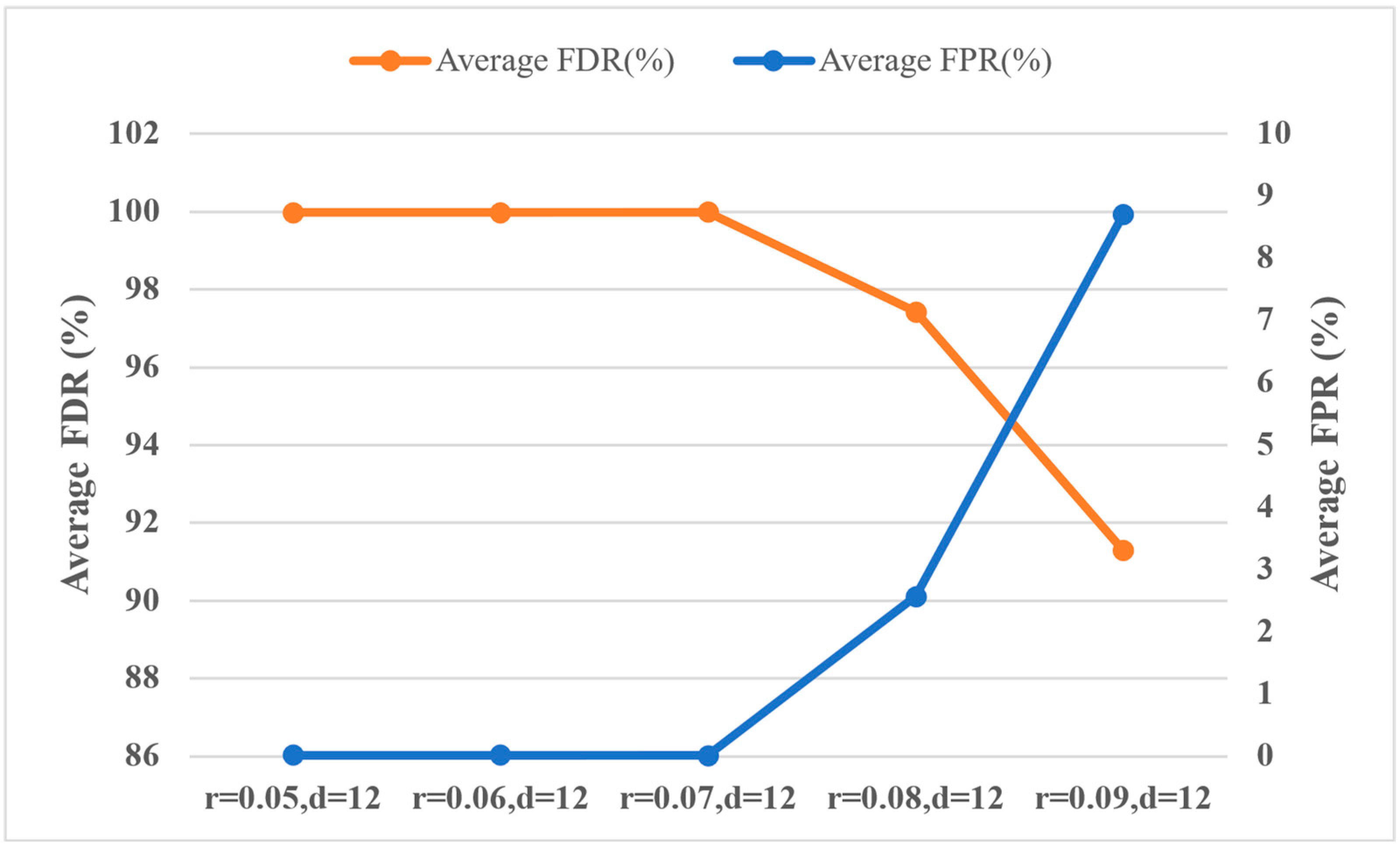
5.3.5. Analysis of Hyperparameter r

We fixed the value of d to its optimal value, namely 12, and selected five different values of r for the analysis of r. The obtained results of $\overline{FDR}$ and $\overline{FPR}$ under different settings of d and r are shown in Figure 7. It can be seen from Figure 7 that the model achieves the best performance on $\overline{FDR}$ and $\overline{FPR}$ when r = 0.07. When r < 0.07, the performance of the model decreases as r decreases. When r > 0.07, the performance of the model decreases as r increases.

The results indicate that there seems to be an intermediate value, r = 0.07, that makes the model perform best when d = 12 is fixed. When r is smaller than the intermediate value, those attributes that are not very relevant to fault diagnosis are also concerned. When r is larger than the intermediate value, only those attributes with great relevance are concerned, which leads to the lack of attention information.

Through the analysis of d and r, one can find that the performance of the model will reach a unique peak at a specific d^∗ and r^∗, assuming that the effects of d and r on model performance are independent of each other. Then, we can fix one parameter and change the value of another to obtain a series of models and evaluate them on the test set. By comparing the evaluation results of the models, d^∗ and r^∗ can be obtained.

5.4. Discussion on the Calculation of Attention Matrix

As indicated in Table 3, the proposed attention layer takes two inputs: the feature map generated by the previous layer and the attention matrix corresponding to the sample. As per Step 3 in Section 3.2, to obtain the attention matrix specific to a particular sample, the knowledge of the label assigned to that sample is indeed required. To be more specific, when we employ the attribute–category attention matrix A(r) to compute the attention matrix associated with a sample, A(r) effectively conveys the category of the sample, given that different categories exhibit distinct attention patterns towards specific attributes. But, the specificity of such conveyance will decrease as the value of r increases. As shown in Figure 8, when the value of r increases, some categories focus on the same attributes, which causes the model to be confused about these categories. Such a requirement of label knowledge makes sense during the training process, but it does not make sense during the testing process, since the model should make predictions based on the input data without any knowledge of the true labels. Notification of label knowledge is equivalent to indirectly revealing the category of the sample to the model, which is why we achieved such good results shown in Table 5.

Nevertheless, the success of the experimental results shows that the integration of reliable prior knowledge into CNNs can greatly improve the accuracy and interpretability of fault diagnosis, which instructs us to seek another definition of prior knowledge that does not depend on labels. In what follows, we present an alternative definition of prior knowledge without relying on labels.

Remember that we ultimately need to obtain the data regions that need to be paid attention to and mark them as 1, while those that do not need to be paid attention to are marked as 0. Considering outliers in the data, it is a fact that the occurrence of faults is always accompanied by outliers. In other words, outliers imply richer fault modes and therefore require special attention. To this end, in step 3 of the proposed method the attention matrix ${\left(A_d^K\right)}_i$ related to a sample $<{\left(S_d^K\right)}_i,{\left(y_m\right)}_i>$ can be obtained through a certain unsupervised outlier detection technique which regards $<{\left(S_d^K\right)}_i,{\left(y_m\right)}_i>$ as the input, such as those presented in the studies [50,51]. In this way, we do not use any label information, and any unsupervised outlier detection technique can be used as an asset to gain prior knowledge for this study.

6. Conclusions and Future Works

We propose an attention-based CNN fault diagnosis method in this study. In the proposal, the integration of prior knowledge about category–attribute correlation based on an attention mechanism significantly improves the accuracy and interpretability of fault diagnosis. A case study in the TE chemical benchmark verifies the effectiveness and superiority of the proposal. Moreover, the conclusion drawn from the sensitivity analysis on hyperparameters provides guidance to set optimal values for hyperparameters. More importantly, we use visualization techniques to analyze the feature extraction process, which shows that the proposal has excellent interpretability. Nevertheless, this study still has the following limitations, which will be solved in our future research.

• This study only validates the effectiveness of the proposal on the TE chemical process dataset; it is necessary to use the proposal to solve other fault diagnosis problems, such as rolling bearing fault diagnosis [52], ice detection of wind turbine blades [53], and gearbox fault diagnosis [54], to further verify the proposal. This is crucial, as it ensures that the proposed method can be easily applied for fault diagnosis in different scenarios.
• This study improves the accuracy and interpretability of fault diagnosis by integrating prior knowledge, but the definition of prior knowledge uses label information, which leads to some irrationality, and thus alternative prior knowledge definitions that do not use label information need to be further studied. A feasible solution is to define the attention matrix as outliers in the data, and then use unsupervised outlier detection methods, such as those presented in [50,51], to obtain the attention matrix.
• Although visualization techniques are used to analyze model interpretability in this study, developing and using quantitative interpretability metrics, such as those presented in the study [55], are worthy of further study for validating the interpretability of the proposed method more specifically.

References

1. Cai, B.; Zhao, Y.; Liu, H.; Xie, M. A Data-Driven Fault Diagnosis Methodology in Three-Phase Inverters for PMSM Drive Systems. IEEE Trans. Power Electron. 2017, 32, 5590–5600. [Google Scholar] [CrossRef]
2. Feng, J.; Yao, Y.; Lu, S.; Liu, Y. Domain Knowledge-based Deep-Broad Learning Framework for Fault Diagnosis. IEEE Trans. Ind. Electron. 2020, 68, 3454–3464. [Google Scholar] [CrossRef]
3. Gao, X.; Hou, J. An improved SVM integrated GS-PCA fault diagnosis approach of Tennessee Eastman process. Neurocomputing 2016, 174, 906–911. [Google Scholar] [CrossRef]
4. Jiang, G.; He, H.; Yan, J.; Xie, P. Multiscale Convolutional Neural Networks for Fault Diagnosis of Wind Turbine Gearbox. IEEE Trans. Ind. Electron. 2019, 66, 3196–3207. [Google Scholar] [CrossRef]
5. Lei, Y.; Jia, F.; Lin, J.; Xing, S.; Ding, S.X. An Intelligent Fault Diagnosis Method Using Unsupervised Feature Learning Towards Mechanical Big Data. IEEE Trans. Ind. Electron. 2016, 63, 3137–3147. [Google Scholar] [CrossRef]
6. He, M.; He, D. Deep Learning Based Approach for Bearing Fault Diagnosis. IEEE Trans. Ind. Appl. 2017, 53, 3057–3065. [Google Scholar] [CrossRef]
7. Jia, F.; Lei, Y.; Lin, J.; Zhou, X.; Lu, N. Deep neural networks: A promising tool for fault characteristic mining and intelligent diagnosis of rotating machinery with massive data. Mech. Syst. Signal Process. 2016, 72–73, 303–315. [Google Scholar] [CrossRef]
8. Shao, H.; Jiang, H.; Wang, F.; Wang, Y. Rolling bearing fault diagnosis using adaptive deep belief network with dual-tree complex wavelet packet. ISA Trans. 2017, 69, 187–201. [Google Scholar] [CrossRef]
9. Liu, H.; Zhou, J.; Zheng, Y.; Jiang, W.; Zhang, Y. Fault diagnosis of rolling bearings with recurrent neural network-based autoencoders. ISA Trans. 2018, 77, 167–178. [Google Scholar] [CrossRef]
10. Wu, H.; Zhao, J. Deep convolutional neural network model based chemical process fault diagnosis. Comput. Chem. Eng. 2018, 115, 185–197. [Google Scholar] [CrossRef]
11. Huang, T.; Zhang, Q.; Tang, X.; Zhao, S.; Lu, X. A novel fault diagnosis method based on CNN and LSTM and its application in fault diagnosis for complex systems. Artif. Intell. Rev. 2022, 55, 1289–1315. [Google Scholar] [CrossRef]
12. Xu, Y.; Li, Z.; Wang, X.; Li, W. Sarkodie-Gyan and S. Feng. A hybrid deep-learning model for fault diagnosis of rolling bearings. Measurement 2021, 169, 108502. [Google Scholar] [CrossRef]
13. Yu, S.; Wang, M.; Pang, S.; Song, L.; Qiao, S. Intelligent fault diagnosis and visual interpretability of rotating machinery based on residual neural network. Measurement 2022, 196, 111228. [Google Scholar] [CrossRef]
14. Li, X.; Zhang, W.; Ding, Q.; Sun, J.Q. Intelligent rotating machinery fault diagnosis based on deep learning using data augmentation. J. Intell. Manuf. 2020, 31, 433–452. [Google Scholar] [CrossRef]
15. Li, C.; Li, S.; Wang, H.; Gu, F.; Ball, A.D. Attention-based deep meta-transfer learning for few-shot fine-grained fault diagnosis. Knowl.-Based Syst. 2023, 264, 110345. [Google Scholar] [CrossRef]
16. Yang, H.; Li, X.; Zhang, W. Interpretability of deep convolutional neural networks on rolling bearing fault diagnosis. Meas. Sci. Technol. 2022, 33, 055005. [Google Scholar] [CrossRef]
17. Yang, D.; Karimi, H.R.; Gelman, L. An explainable intelligence fault diagnosis framework for rotating machinery. Neurocomputing 2023, 541, 126257. [Google Scholar] [CrossRef]
18. Li, X.; Zhang, W.; Ding, Q. Understanding and improving deep learning-based rolling bearing fault diagnosis with attention mechanism. Signal Process. 2019, 161, 136–154. [Google Scholar] [CrossRef]
19. Yu, J.; Liu, G. Knowledge extraction and insertion to deep belief network for gearbox fault diagnosis. Knowl.-Based Syst. 2020, 197, 105883. [Google Scholar] [CrossRef]
20. Xie, T.; Xu, Q.; Jiang, C.; Lu, S.; Wang, X. The fault frequency priors fusion deep learning framework with application to fault diagnosis of offshore wind turbines. Renew. Energ. 2023, 202, 143–153. [Google Scholar] [CrossRef]
21. Liao, J.; Dong, H.; Sun, Z.; Sun, J.; Zhang, S.; Fan, F. Attention-embedded quadratic network (qttention) for effective and interpretable bearing fault diagnosis. IEEE Trans. Instrum. Meas. 2023, 72, 1–13. [Google Scholar] [CrossRef]
22. Peng, D.; Wang, H.; Desmet, W.; Gryllias, K. RMA-CNN: A residual mixed-domain attention CNN for bearings fault diagnosis and its time-frequency domain interpretability. J. Dyn. Monit. Diagn. 2023, 2, 115–132. [Google Scholar] [CrossRef]
23. Yin, S.; Ding, S.X.; Haghani, A.; Hao, H.; Zhang, P. A comparison study of basic data-driven fault diagnosis and process monitoring methods on the benchmark Tennessee Eastman process. J. Process Control 2012, 22, 1567–1581. [Google Scholar] [CrossRef]
24. Girshick, R.; Donahue, J.; Darrell, T.; Malik, J. Rich feature hierarchies for accurate object detection and semantic segmentation. In Proceedings of the IEEE Conference on Computer Vision and Pattern Recognition, Columbus, OH, USA, 23–28 June 2014; pp. 580–587. [Google Scholar]
25. Girshick, R. Fast r-cnn. In Proceedings of the IEEE International Conference on Computer Vision, Santiago, Chile, 11–18 December 2015; pp. 1440–1448. [Google Scholar]
26. Ren, S.; He, K.; Girshick, R.; Sun, J. Faster r-cnn: Towards real-time object detection with region proposal networks. In Proceedings of the Advances in Neural Information Processing Systems 28 (NIPS 2015), Montreal, QC, Canada, 7–12 December 2015; Volume 28. [Google Scholar]
27. He, K.; Gkioxari, G.; Dollár, P.; Girshick, R. Mask r-cnn. In Proceedings of the IEEE International Conference on Computer Vision, Venice, Italy, 22–29 October 2017; pp. 2961–2969. [Google Scholar]
28. Uijlings, J.R.; Van De Sande, K.E.; Gevers, T.; Smeulders, A.W. Selective search for object recognition. Int. J. Comput. Vision 2013, 104, 154–171. [Google Scholar] [CrossRef]
29. Qi, L.; Huo, J.; Wang, L.; Shi, Y.; Gao, Y. A mask based deep ranking neural network for person retrieval. In Proceedings of the IEEE International Conference on Multimedia and Expo (ICME), Shanghai, China, 8–12 July 2019; pp. 496–501. [Google Scholar]
30. Liu, L.Y.F.; Liu, Y.; Zhu, H. Masked convolutional neural network for supervised learning problems. Stat 2020, 9, e290. [Google Scholar] [CrossRef] [PubMed]
31. Cai, L.; Li, H.; Dong, W.; Fang, H. Micro-expression recognition using 3D DenseNet fused Squeeze-and-Excitation Networks. Appl. Soft Comput. 2022, 119, 108594. [Google Scholar] [CrossRef]
32. Roy, S.K.; Dubey, S.R.; Chatterjee, S.; Chaudhuri, B.B. FuSENet: Fused squeeze-and-excitation network for spectral-spatial hyperspectral image classification. IET Image Process. 2020, 14, 1653–1661. [Google Scholar] [CrossRef]
33. Hu, J.; Shen, L.; Sun, G. Squeeze-and-excitation networks. In Proceedings of the IEEE Conference on Computer Vision and Pattern Recognition, Salt Lake City, UT, USA, 18–22 June 2018; pp. 7132–7141. [Google Scholar]
34. Krizhevsky, A.; Sutskever, I.; Hinton, G.E. ImageNet Classification with Deep Convolutional Neural Networks. In Advances in Neural Information Processing Systems 25; Pereira, F., Burges, C.J.C., Bottou, L., Weinberger, K.Q., Eds.; Curran Associates, Inc.: Red Hook, NY, USA, 2012; pp. 1097–1105. [Google Scholar]
35. Wei, W.W. Multivariate Time Series Analysis and Applications; John Wiley & Sons: Hoboken, NJ, USA, 2018. [Google Scholar]
36. Vaswani, A.; Shazeer, N.; Parmar, N.; Uszkoreit, J.; Jones, L.; Gomez, A.N.; Kaiser, Ł.; Polosukhin, I. Attention is All you Need. In Advances in Neural Information Processing Systems 30; Guyon, I., Luxburg, U.V., Bengio, S., Wallach, H., Fergus, R., Vishwanathan, S., Garnett, R., Eds.; Curran Associates, Inc.: Red Hook, NY, USA, 2017; pp. 5998–6008. [Google Scholar]
37. Yu, Z.; Peng, W.; Li, X.; Hong, X.; Zhao, G. Remote heart rate measurement from highly compressed facial videos: An end-to-end deep learning solution with video enhancement. In Proceedings of the 2019 IEEE/CVF International Conference on Computer Vision (ICCV), Seoul, Republic of Korea, 27 October–2 November 2019; pp. 151–160. [Google Scholar]
38. Puth, M.T.; Neuhäuser, M.; Ruxton, G.D. Effective use of Pearson’s product–moment correlation coefficient. Anim. Behav. 2014, 93, 183–189. [Google Scholar] [CrossRef]
39. Cohen, J. Statistical Power Analysis for the Behavioral Sciences; Academic Press: Cambridge, MA, USA, 2013. [Google Scholar]
40. Downs, J.J.; Vogel, E.F. A plant-wide industrial process control problem. Comput. Chem. Eng. 1993, 17, 245–255. [Google Scholar] [CrossRef]
41. He, H.; Garcia, E.A. Learning from Imbalanced Data. IEEE Trans. Knowl. Data Eng. 2009, 21, 1263–1284. [Google Scholar]
42. Ioffe, S.; Szegedy, C. Batch Normalization: Accelerating deep network training by reducing internal covariate shift. arXiv 2015, arXiv:1502.03167. [Google Scholar]
43. Srivastava, N.; Hinton, G.; Krizhevsky, A.; Sutskever, I.; Salakhutdinov, R. Dropout: A simple way to prevent neural networks from overfitting. J. Mach. Learn. Res. 2014, 15, 1929–1958. [Google Scholar]
44. Kingma, D.P.; Ba, J. Adam: A method for stochastic optimization. arXiv 2017, arXiv:1412.6980. [Google Scholar]
45. Zeiler, M.D.; Fergus, R. Visualizing and understanding convolutional networks. In Proceedings of the European Conference on Computer Vision, Zurich, Switzerland, 6–12 September 2014; pp. 818–833. [Google Scholar]
46. Olden, J.D.; Jackson, D.A. Illuminating the “black box”: A randomization approach for understanding variable contributions in artificial neural networks. Ecol. Model. 2002, 154, 135–150. [Google Scholar] [CrossRef]
47. Lv, F.; Wen, C. Fault Diagnosis Based on Deep Learning. In Proceedings of the 2016 American Control Conference (ACC), Boston, MA, USA, 6–8 July 2016; pp. 6851–6856. [Google Scholar]
48. Wang, Y.; Pan, Z.; Yuan, X.; Yang, C.; Gui, W. A novel deep learning based fault diagnosis approach for chemical process with extended deep belief network. ISA Trans. 2020, 96, 457–467. [Google Scholar] [CrossRef]
49. Jing, C.; Hou, J. SVM and PCA based fault classification approaches for complicated industrial process. Neurocomputing 2015, 167, 636–642. [Google Scholar] [CrossRef]
50. Samariya, D.; Thakkar, A. A comprehensive survey of anomaly detection algorithms. Ann. Data Sci. 2023, 10, 829–850. [Google Scholar] [CrossRef]
51. Smiti, A. A critical overview of outlier detection methods. Comput. Sci. Rev. 2020, 38, 100306. [Google Scholar] [CrossRef]
52. Li, B.; Chow, M.-Y.; Tipsuwan, Y.; Hung, J.C. Neural-network-based motor rolling bearing fault diagnosis. IEEE Trans. Ind. Electron. 2000, 47, 1060–1069. [Google Scholar] [CrossRef]
53. Du, Y.; Zhou, S.; Jing, X.; Peng, Y.; Wu, H.; Kwok, N. Damage detection techniques for wind turbine blades: A review. Mech. Syst. Signal Process. 2020, 141, 106445. [Google Scholar] [CrossRef]
54. Cheng, W.; Wang, S.; Liu, Y.; Chen, X.; Nie, Z.; Xing, J.; Zhang, R.; Huang, Q. A novel planetary gearbox fault diagnosis method for nuclear circulating water pump with class imbalance and data distribution shift. IEEE Trans. Instrum. Meas. 2023, 72, 1–13. [Google Scholar] [CrossRef]
55. Vilone, G.; Longo, L. Notions of explainability and evaluation approaches for explainable artificial intelligence. Inform. Fusion 2021, 76, 89–106. [Google Scholar] [CrossRef]
Figure 1. SWP W ( d , λ ) for the raw time series S T K and Y T M .
Processes 11 03233 g001
Figure 2. The process of integrating prior knowledge into CNNs.
Processes 11 03233 g002
Figure 3. Method of calculating attention matrix ( A d K ) i related to a sample < ( S d K ) i , ( y m ) i > . t δ indicates the time when the fault f m occurs and c 1 ~ , c 2 ~ = { arg c k a m k = 1 | k = 1 , , K ; a m k A r } . The gray squares in ( A d K ) i are equal to 1; others are equal to 0.
Processes 11 03233 g003
Figure 4. Visible feature extraction process of S d K i and S d K j that have the same category.
Processes 11 03233 g004
Figure 5. Visible feature extraction process of S d K i and S d K j that have different categories but the same prior knowledge.
Processes 11 03233 g005
Figure 6. Average FDR and FPR obtained by models with a fixed r = 0.07 and different d (2, 12, 32, 52, 72).
Processes 11 03233 g006
Figure 7. Average FDR and FPR obtained by models with a fixed d = 12 and different r (0.05, 0.06, 0.07, 0.08, 0.09).
Processes 11 03233 g007
Figure 8. Visualization of category–attribute attention matrix A(r) with different r.
Processes 11 03233 g008