Numerical Study on the Influence of Different Operating Conditions on Mixing Uniformity of the Helical Gear Pump Mixer

Abstract

The uniformity of the gelatin solution and water mixing process is a critical factor in the performance of helical gear pump mixers that affects pump efficiency. In this study, we investigate the impact of water inlet velocity and rotational speed on the helical gear pump mixer. A numerical model of the helical gear pump mixer is established using Simerics MP+ 5.2.15 software. By varying the water inlet velocity from 0.159 m/s to 1.272 m/s and the rotational speed from 8 rpm to 50 rpm, we obtained volume fraction distributions of water in different sections of the helical gear pump mixer. The simulation results show that the high water inlet velocity causes the water and gelatin solution in the mixing tank to not mix fully. When the inlet speed is 0.318 m/s, the mixing uniformity of the gelatin solution and water in the mixing tank is effectively promoted, and the maximum volume fraction of water in the water-rich region is reduced by 70.24%. In poor water regions, the maximum volume fraction of water increased by 9.25 times. Furthermore, within a certain range, increasing the rotational speed of the helical gear pump promotes the faster transport of water to the back of the mixing tank, leading to reduced non-uniformity in the gelatin solution and water mixing process. These findings provide valuable insights for enhancing mixing uniformity in helical gear pump mixers.

1. Introduction

The helical gear pump has the characteristics of low flow pulsation, high efficiency, and low meshing vibration [1]. Therefore, it is widely used in high-pressure transportation, food processing, pharmaceutical manufacturing, and other fields [2,3]. For example, in the production of drug capsule shells, a helical gear pump is often used for the mixing and transportation of gelatin solution, which is a common capsule shell material with high viscosity [4]. The gelatin solution is filled in the helical gear pump during the production of the capsule shell and is diluted with water if the viscosity of the gelatin solution is too high. Uneven mixing of the two phases leads to significant changes in the viscosity of the gelatin solution, thereby reducing the work efficiency [5,6]. Therefore, analyzing the volume fraction distribution of water in the gelatin solution under different operating conditions is urgently needed to improve the uniformity of the two-phase mixing process and ensure work efficiency [7].

Since the development of the intricate geometric configuration of the helical gear pump mixer, the investigation of its flow field has faced great challenges. Some researchers have tried to adopt experimental methodologies to observe the flow characteristics of helical gear pumps [8,9,10,11]. Although experimental testing can directly provide on-site data, the experimental process is costly and the analysis ability of the internal flow field of helical gear pumps is usually insufficient via experimental methods. Computational fluid dynamics (CFD) simulation technology has been widely used for analyzing the flow characteristics of external gear pumps [12,13,14]. The flow field of a spur gear pump was numerically simulated by Li using dynamic mesh and volume of fluid (VOF) methods [15]. The results revealed that the distribution of internal lubricating oil and gas is significantly influenced by high rotational speed. Ji conducted a numerical simulation using the smooth particle hydrodynamics (SPH) method to investigate oil and gas two-phase flow in a spur gear pump [16]. Their findings demonstrated that the gear tip velocity played a dominant role in generating splashes. Additionally, the numerical simulation of three-phase flow in a spur gear pump was conducted by Mithun et al. employing the immersed solid method (ISM) [17,18]. The findings indicated that the increase in rotational speed led to an augmentation in cavitation intensity within the pump. These studies mainly focus on conventional external gear pumps.

For the helical gear pump mixer, the gear meshing clearance is small and has a helical angle. This makes simulating a helical gear pump mixer extremely difficult and time-consuming. Under the current conditions, Zhao proposed a multi-domain dynamic simulation model of a helical gear pump, which can accurately predict the vibration and friction wear of gears [19]. However, this is only applicable to the specific shape of the helical gear pump. Salawu conducted a numerical simulation study on the power loss of the gearbox of the helical gear pump [20]. The findings revealed that the friction between the gears significantly influenced the power loss of the gearbox. But their method could not analyze the internal flow field. Zhou conducted a numerical simulation on the oil injection process of a high-speed helical gear pump based on the overset mesh method [21], and the research results showed that the inlet velocity was positively correlated with the distribution of the volume fraction of oil on the tooth surface. It should be noted that the overset mesh just mentioned can easily produce orphan cells, which are extremely difficult to handle. These studies mainly focus on the effects of friction and wear, flow pulsation, and oil distribution on the helical gear pump. There is no research on the mixing uniformity of the two-phase flow field of the helical gear pump. Furthermore, the above methods have some limitations. To solve this problem, Simerics MP+ 5.2.15 provides a universal helical gear pump template, which can generate structured grids for the entire helical gear pump area, greatly reducing the number of grids and calculation time, and has been verified to have good reliability [22].

There is an absence of research on the two-phase flow field of gelatin solution and water in helical gear pump mixers. Such research is necessary in order to improve the uniformity of the two-phase mixing of gelatin solution and water in helical gear pump mixers. In this paper, a numerical model of a helical gear pump mixer was established by using Simerics MP+ based on the VOF two-phase flow model and moving/sliding method, fully taking account of the influence of narrow gear clearance and the helical angle of the helical gear pump, as well as the interaction of the gelatin solution and water two-phase flow. The simulation results were validated using on-site experimental data. Numerical simulations were performed to investigate the mixing process of gelatin solution and water in a helical gear pump mixer. The influence of different inlet velocities and rotational speeds on the mixing uniformity of the two-phase flow field in the helical gear pump mixer was analyzed. These results are helpful in improving the two-phase mixing uniformity of helical gear pump mixers and their working efficiency.

2. Numerical Model

2.1. CFD Model

The helical gear pump mixer investigated in this study is primarily utilized for the mixed transportation of gelatin solution and water. The geometric model of the fluid domain was established according to the helical gear pump mixer. As shown in Figure 1a, the helical gear pump mixer consists of a driving gear, a driven gear, a deflector, and a mixing tank. The number of teeth of the driving wheel and the driven wheel is 8. The driving gear rotates in a clockwise direction, while the driven gear rotates counterclockwise. As shown in Figure 1b, the gelatin solution inlets the helical gear pump through seven inlets at the bottom. Water is injected through the front face of the helical gear pump, and the diameter of the water inlet is 4 mm. As shown in Figure 1c, to ensure domain connectivity and prevent negative volumes, there is a gap between the driving gear and the driven gear in the gear meshing area, and the high and low pressure chambers are connected. The center distance is 51 mm, the gear meshing clearance is 0.05 mm, and the clearance between the gear and the chamber is 0.1 mm. As shown in Figure 1d, the tooth width of the helical gear pump measures 665 mm, while the deflector has dimensions of 50 mm in height and 646 mm in length.

2.2. Grid Division and Grid Independence Verification

The helical gear pump mixer is initially filled with gelatin solution, with a density of 1090 kg/m³ and a viscosity of 0.45$\mathrm{Pa}·\mathrm{s}$, while the density of water is 998 kg/m³ and the viscosity of water is 0.0003565 $\mathrm{Pa}·\mathrm{s}$. The temperature of the gelatin solution is kept at 45 °C and the water temperature is 80 °C. When the gear rotates, the mixture of gelatin solution and water is driven by the helical gear. Part of the mixture is transported backward under the axial force of the helical gear, while the other part is driven by the radial force of the helical gear and enters the mixing tank through the tooth tip clearance along the deflector.

Table 1. Helical gear pump working parameter.

Parameter	Driving Wheel, Driven Wheel
Gear teeth$z_1$	8
Normal module $m_{n }$(mm)	6.35
Normal pressure angle ${\alpha }_n$(°)	20
Spiral angle $\beta (°)$	8
Center distance $c$(mm)	51
Tooth width$B_1$(mm)	665
Rotational speed $n_1$(rpm)	8, 20, 30, 40, 50

gives the detailed operating parameters of the helical gear pump. The driving wheel and the driven wheel have the same parameters.

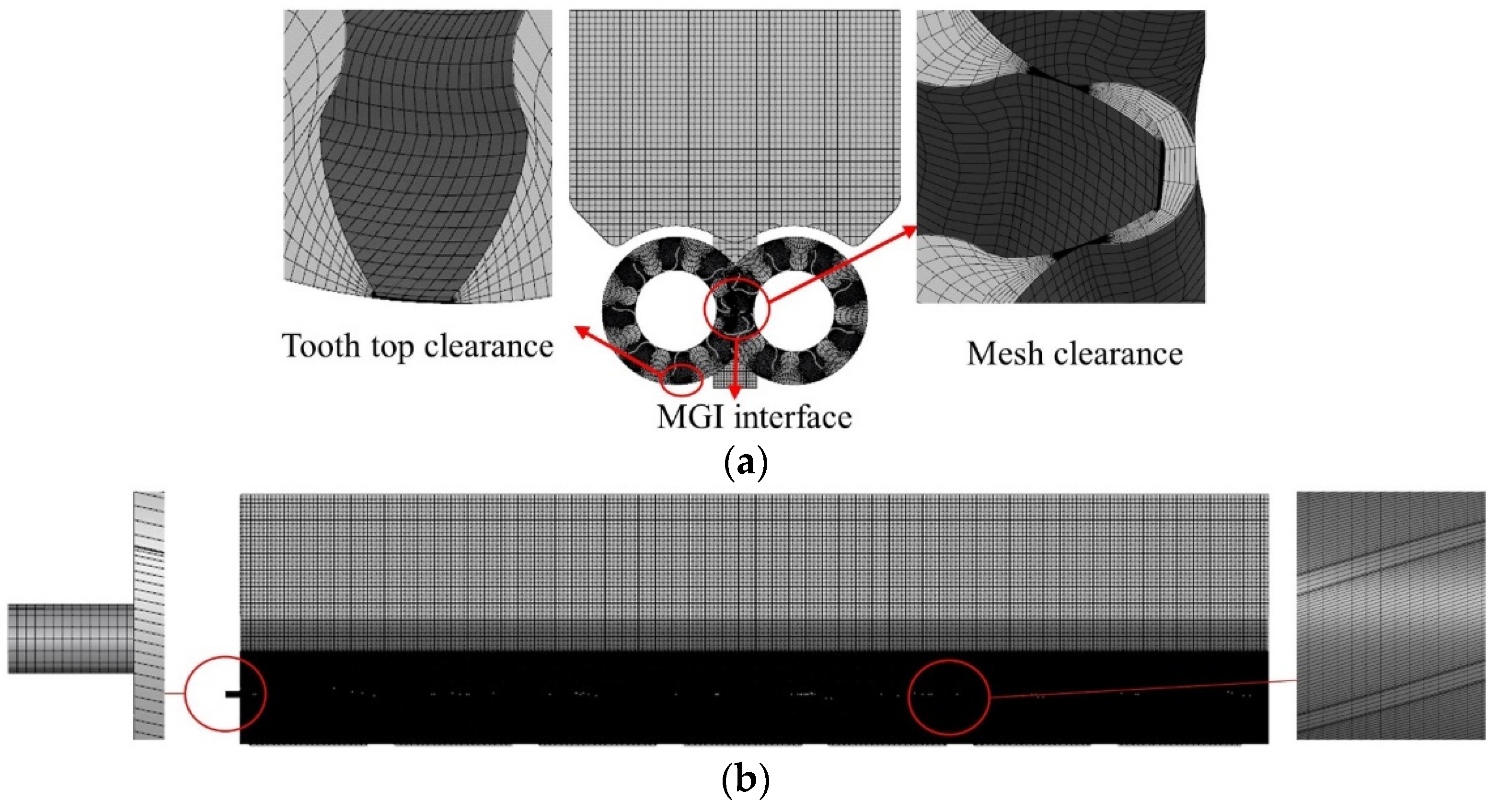
The helical gear pump mixer computational domain is composed of structured mesh. The driving wheel and the driven wheel are connected by the mismatched grid interfaces (MGIs). As shown in Figure 2, due to the drastic changes in the velocity field and pressure field of the inlet area, the area of the inlet is locally encrypted. In order to ensure that the calculation results are not affected by the number of grids, it is necessary to perform grid independence verification to obtain the most appropriate grid number. The average mass flow rate over a working cycle (12 s) was evaluated by taking the number of grid units as the independent variable. As shown in

Table 2. Grid independence verification.

Cases	Total Mesh Elements	Average Mass Rate (kg/s)
1	1,196,228	0.002716
2	1,436,823	0.003820
3	1,757,316	0.003907
4	2,075,991	0.003916

, the average mass flow rate of the mixed tank in four cases was compared. When the number of grids increased to case 3, the outlet mass flow rate tended to stabilize. Therefore, in all subsequent simulations, the number of grid cells was limited to 1.75 million.

2.3. Governing Equation

In this study, the conservation equations for mass and momentum were discretized using the finite volume method. These conservation equations can be expressed as integrals in the following forms [23]:

$$\frac{\partial }{\partial t}{{\displaystyle \int }}_{{\Omega }_{\left(t\right)}}^{ }\rho d\Omega +{{\displaystyle \int }}_{\sigma }^{ }\rho \left(\mathit{v}-{\mathit{v}}_{\sigma }\right)\mathit{n}d\sigma =0,$$

(1)

$$\frac{\partial }{\partial t}{{\displaystyle \int }}_{{\Omega }_{\left(t\right)}}^{ }\rho \mathit{v}d\Omega +{{\displaystyle \int }}_{\sigma }^{ }\rho \left(\left(\mathit{\nu }-{\mathit{\nu }}_{\sigma }\right)\mathit{n}\right)\mathit{v}d\sigma ={{\displaystyle \int }}_{\sigma }^{ }\tilde{\mathit{\tau }}\mathit{n}d\sigma -{{\displaystyle \int }}_{\sigma }^{ }p\mathit{n}d\sigma +{{\displaystyle \int }}_{\Omega }^{ }\mathit{f}d\Omega ,$$

(2)

where ${\Omega }_{\left(t\right)}$ is the volume of the computational domain, $\sigma$ is the surface of the computational domain volume ${\Omega }_{\left(t\right)}$, $\mathit{n}$ is the outward pointing normal of the surface of σ, $\rho$ is the weighted fluid density, $p$ is the pressure, $\mathit{f}$ is the body force, $\mathit{v}$ is the fluid velocity, $\tilde{\mathit{\tau }}$ is shear stress tensor, and $v_{\sigma }$ is the velocity of the surface motion.

The standard k-$\epsilon$ model is used for turbulence calculation. As the most widely used turbulence model, the standard k-$\epsilon$turbulence model has better convergence than other turbulence models. It is the optimal choice for analyzing current models and does not differ significantly from other models in calculating flows. The standard k-$\epsilon$ model is based on the following two equations:

$$\frac{\partial }{\partial t}{{\displaystyle \int }}_{{\Omega }_{\left(t\right)}}^{ }\rho kd\Omega +{{\displaystyle \int }}_{\sigma }^{ }\rho \left(\left(\mathit{\nu }-{\mathit{\nu }}_{\sigma }\right)\mathit{n}\right)kd\sigma ={{\displaystyle \int }}_{\sigma }^{ }\left(\mu +\frac{{\mu }_t}{{\sigma }_k}\right)\left(\nabla k\mathit{n}\right)d\sigma +{{\displaystyle \int }}_{\Omega }^{ }\left(G_t-\rho \epsilon \right)d\sigma ,$$

(3)

$$\frac{\partial }{\partial t}{{\displaystyle \int }}_{{\Omega }_{\left(t\right)}}^{ }\rho \epsilon d\Omega +{{\displaystyle \int }}_{\sigma }^{ }\rho \left(\left(\mathit{\nu }-{\mathit{\nu }}_{\sigma }\right)\mathit{n}\right)\epsilon d\sigma ={{\displaystyle \int }}_{\sigma }^{ }\left(\mu +\frac{{\mu }_t}{{\sigma }_{\epsilon }}\right)\left(\nabla \epsilon \mathit{n}\right)d\sigma +{{\displaystyle \int }}_{\Omega }^{ }\left(c_1{G}_t\frac{\epsilon }{k}-c_2\rho \frac{{\epsilon }^2}{k}\right)d\Omega ,$$

(4)

In the above formula,$c_1$= 1.44, $c_2$= 1.92, ${\sigma }_k$=1, and ${\sigma }_{\epsilon }$ = 1.3. Where ${\sigma }_k$ and ${\sigma }_{\epsilon }$ are the reciprocals of the Prandtl numbers of $k$ and $\epsilon$, $k$ is the turbulent kinetic energy, $\epsilon$ is the dissipation rate of turbulent kinetic energy, $\rho$ is the fluid density, $\mu$ is the dynamic viscosity of the fluid, and ${\mu }_t$ is the turbulent viscosity of turbulent kinetic energy diffusion.

The VOF model developed by Hirt [24] has been widely used in the simulation of two-phase flow. This model has been proved by Scardovelli to be an effective tool for analyzing the volume fraction distribution of different fluids in two-phase flow [25]. The VOF model represents the volume fraction occupied by each fluid component in each cell by solving a set of scalar transport equations. The transfer equation for the volume fraction of each fluid component can be written as:

$$\frac{\partial }{\partial t}{{\displaystyle \int }}_{{\Omega }_{\left(t\right)}}^{ }{\rho }_i{F}_{i}d\Omega +\underset{\sigma }{\overset{ }{{\displaystyle \int }}}{\rho }_i\left(v-v_{\sigma }\right)n{F}_{i}d\sigma =0,$$

(5)

where $F_i$ is the volume fraction of phase $i$ fluid and ${\rho }_i$ is the density of phase $i$ fluid. The density of the fluid mixture in Equations (1)–(5) is:

$$\rho ={{\displaystyle \sum }}^{ }{\rho }_i{F}_i,$$

(6)

The high-resolution interface capture (HRIC) scheme is employed to handle convection terms in transport equations, while the current VOF model was verified to be suitable for two-phase flow without the energy equation [26].

The gelatin solution is a Newtonian fluid at 45 °C. For a Newtonian fluid, the shear stress tensor $\tilde{\mathit{\tau }}$ is a function of the fluid viscosity and velocity gradient given by the following equation:

$${\tau }_{ij}=\mu \left(\frac{\partial {\mu }_i}{\partial x_j}+\frac{\partial {\mu }_j}{\partial x_i}\right)-\frac{2}{3}\mu \frac{\partial {\mu }_k}{\partial x_k}{\delta }_{ij},$$

(7)

where ${\mu }_i$(i = 1,2,3) is the velocity component and ${\delta }_{ij}$ is Kronecker delta function.

2.4. Boundary Conditions

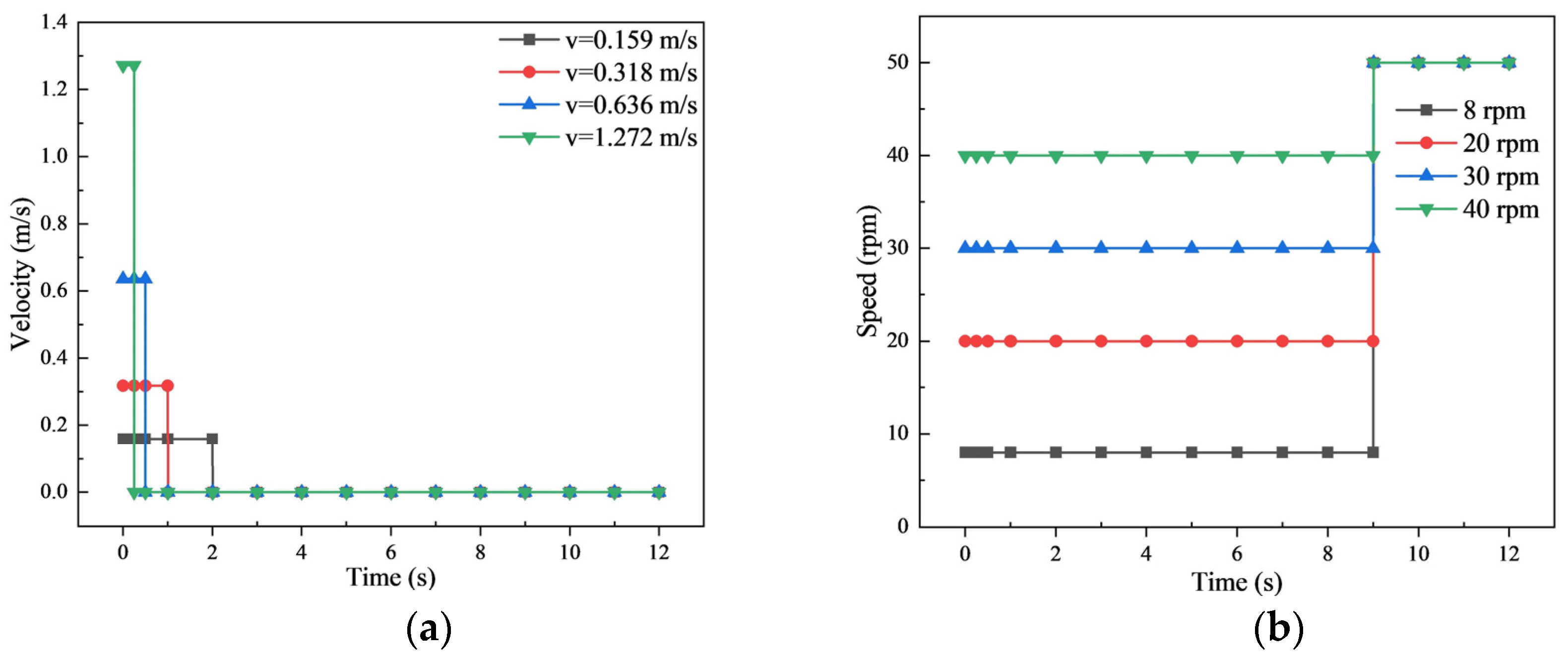
In the actual working process of the helical gear pump mixer, the mixing tank is filled with gelatin solution, and water needs to be added regularly to ensure the stability of the gelatin solution’s viscosity. A working cycle of the helical gear pump mixer is 12 s, 0 to 9 s gear for low-speed operation, and 9 to 12 s gear for high-speed operation. When the time is 0 s, water starts to enter. As shown in Figure 3, in the simulation process, the water inlet velocity and rotation speed are controlled by the edited expression. The rotation speed and outlet boundary conditions are shown in Figure 4a. The inlet velocity boundary conditions are shown in Figure 4b.

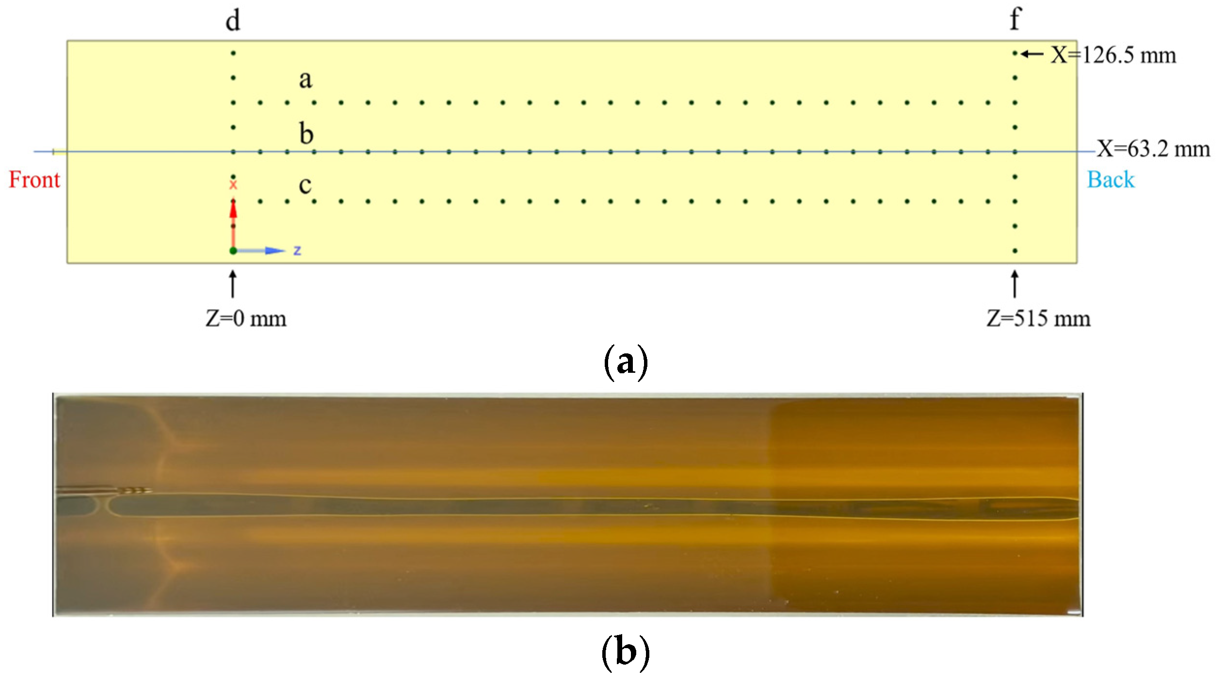
The operation condition of the helical gear pump in one cycle is numerically simulated. The time step of all unsteady simulations is 0.01 s. As shown in Figure 5a, according to actual production conditions, six monitoring lines a, b, c, d and f are set at the outlet section to monitor the distribution of the water volume fraction in real time. The change in the volume fraction of the water was recorded at different times. Figure 5b shows the actual outlet cross-section.

3. Results and Discussion

3.1. Model Reliability Verification

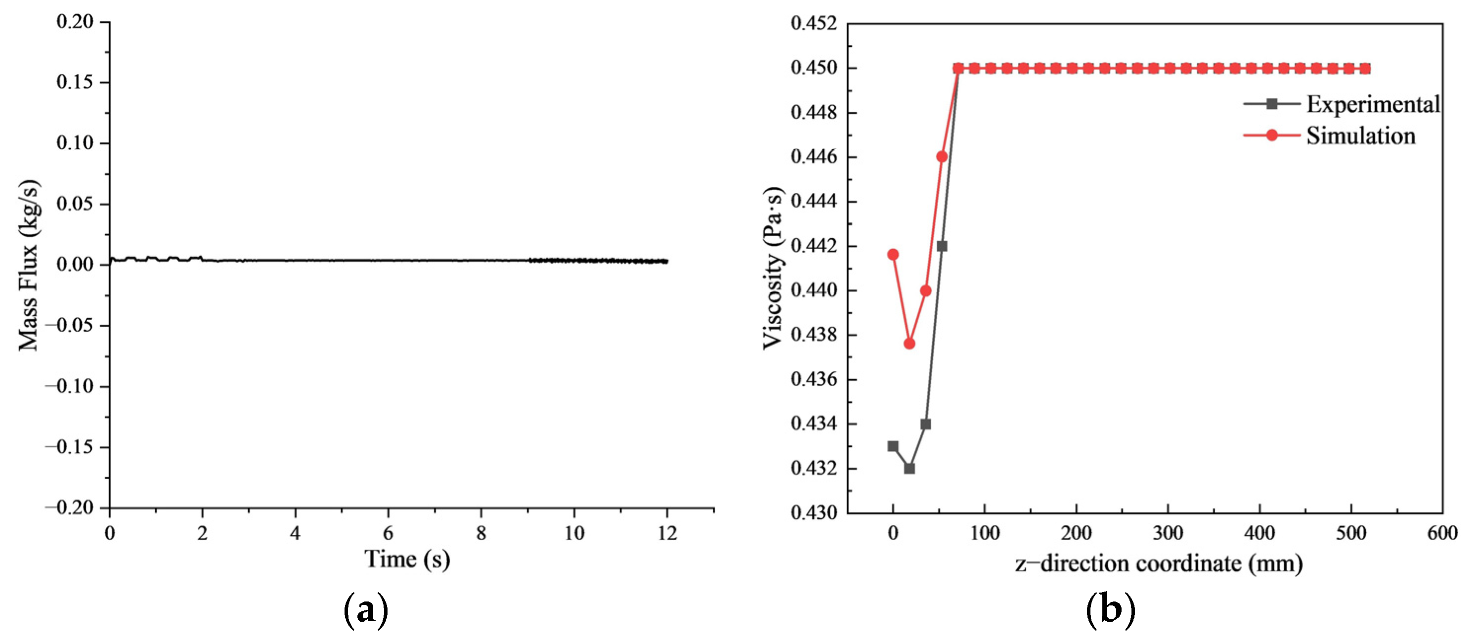
Based on the actual model of the helical gear pump mixer, the numerical simulation is carried out under the same working conditions. The working cycle of the helical gear pump mixer is 12 s, the 0 to 9 s gear speed is 8 rpm, and the 9 to 12 s gear speed is 50 rpm. The water inlet velocity is 0.636 m/s. The gelatin solution inlet velocity is 0.00034 m/s. As shown in Figure 6a, the outlet cross-section mass flow rate is regularly monitored and a large number of iterations are carried out in the simulation to keep the mass flow flux stable. According to the set monitoring point, the outlet cross-section viscosity of the mixer tank was measured after one cycle of operation. The data on the monitoring line b in Figure 5a were extracted, and the actual viscosity of the corresponding points was measured using a rotary rheometer. By comparing the experimental data with the simulation data, we can see from Figure 6b that the error range is 0.9 % to 1.9 %. These results verify the authenticity of the helical gear pump mixer simulation. The gap between the model data and the experimental data is due to the fact that the model does not consider the effect of temperature on the two-phase flow of gelatin solution and water, as well as the effect of friction and wear of the gear itself.

3.2. Effect of Inlet Velocity on Mixing Uniformity in a Helical Gear Pump Mixer

As shown in

Table 3. Different water inlet velocity conditions.

Case	Water Inlet (m/s)	Time (s)
a	0.159	2
b	0.318	1
c	0.636	0.5
d	1.272	0.25

, the mixing of gelatin solution/water in a working cycle of the helical gear pump mixer was analyzed. As shown in Figure 7a, the volume fraction distribution of water in different cross-sections of the helical gear pump mixer was determined under four different water inlet velocities (0.159 m/s, 0.318 m/s, 0.636 m/s, and 1.272 m/s). Since the water inlet is located on the front surface of the helical gear pump, when the water enters the helical gear pump area, the presence of the helix angle causes part of the water to be transported in the positive direction along the z-axis. The other part of the water is transported in the positive direction along the y-axis, passes through the deflector plate, and enters the gelatin solution and water mixing tank area. Therefore, the water is first discharged from the front end of the mixing tank outlet. Under the four different water inlet velocities, the distribution trend of the water volume fraction at the outlet section of the mixing tank is consistent. The front end of the outlet forms a water-rich region, and the volume fraction of water in other areas of the outlet forms a water-poor region. As shown in Figure 7b, we amplified the volume fraction of water at the outlet cross-section. The volume fraction of water in the water-poor region is observed to increase proportionally with the water inlet velocity. However, when the water inlet velocity is increased to 1.272 m/s, the distribution of water is mainly concentrated in the middle and both sides of the outlet cross-section, which is not conducive to improving the mixing uniformity.

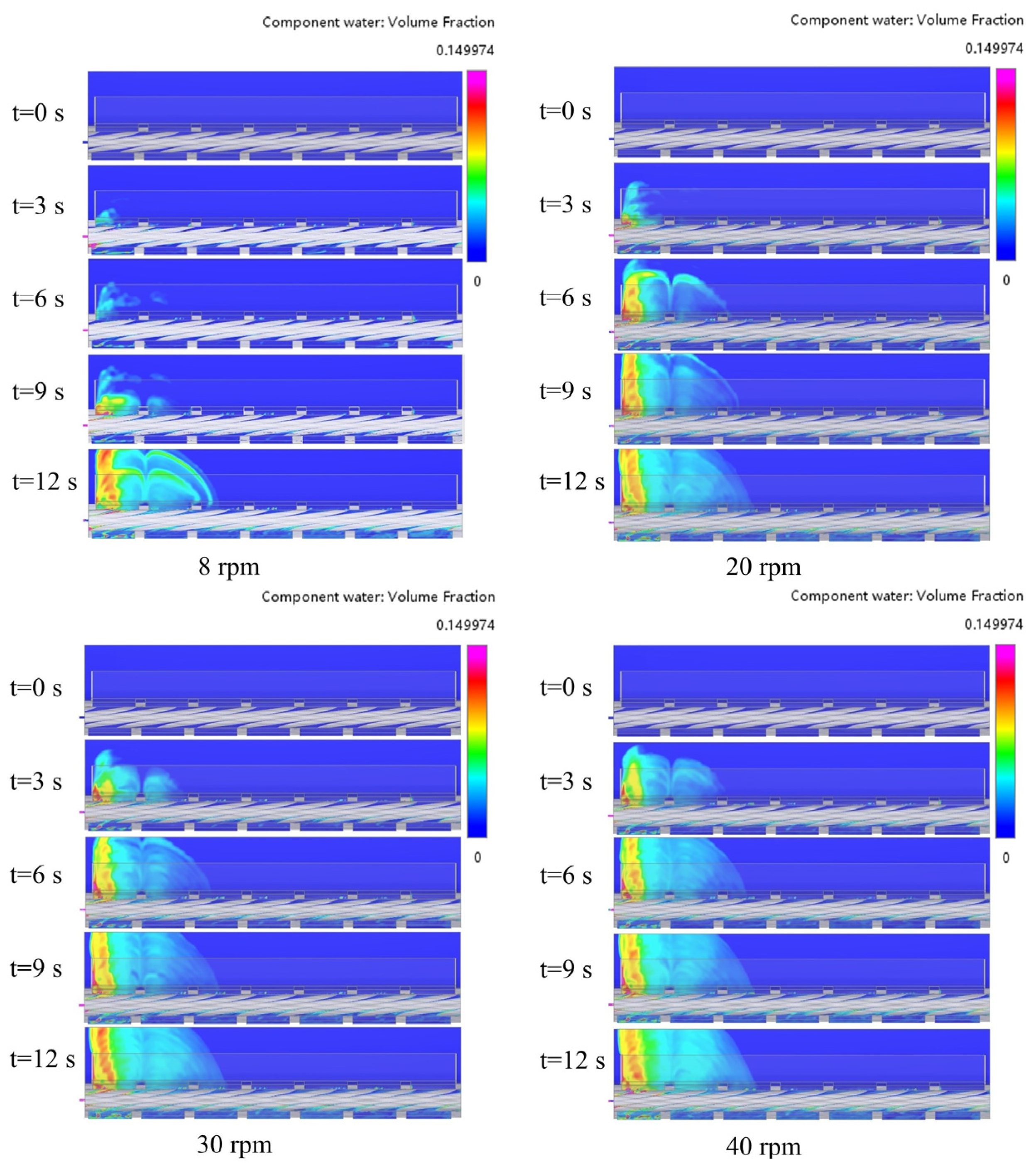
Figure 8 shows the water distribution at the x = 63.2 mm outlet cross-section under different water inlet velocities. With the rotation of the gear, the water is gradually transported to the back of the mixing tank, and the water is mainly distributed in the mixing tank area above the first and second gelatin solution inlet. When the velocity is 0.159 m/s, due to the small water inlet velocity, the volume fraction of water in the mixing tank area above the first gelatin solution inlet is larger than that at other gelatin solution inlet velocities. When the water inlet velocity is greater than 0.318 m/s, as the inlet velocity continues to increase, the time for water to reach the back end of the mixing tank is reduced, but since 0 to 9 s is a low rotation speed, this causes more water to concentrate in the front end of the mixing tank, and the volume fraction of water in the front end of the mixing tank is larger, which is not conducive to the uniform distribution of water in the mixing tank.

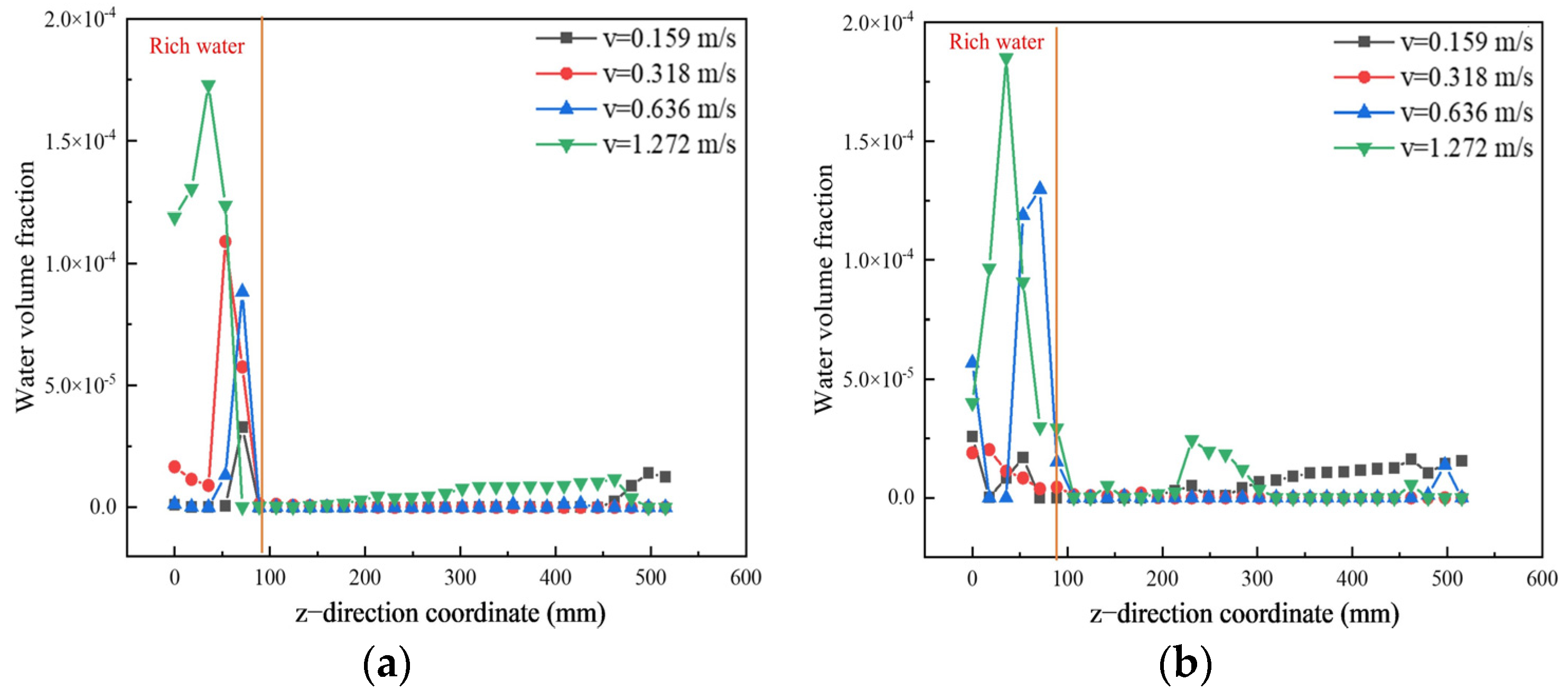
Figure 9a shows the distribution of water volume fractions at monitoring line b. It can be observed from the figure that when the z-axis position is less than 88 mm, the distribution of water is relatively dense, forming a water-rich region. Moving in the positive direction of the z-axis, the volume fraction of water first increases and then decreases. The volume fraction of water in the water-rich region increases with the increase in water inlet velocity. As shown in Figure 9b, when the z value is greater than 88 mm, the volume fraction of water near the back end of the outlet is larger. Especially when the inlet speed is 0.318 m/s, the distribution of the water volume fraction is the largest at the end and the smallest at the front. This shows that when the water inlet speed is 0.318 m/s, the water is delivered more quickly to the back of the mixing tank, and does not accumulate in the water-rich region, which is conducive to improving the uniformity of the two-phase mixing of gelatin solution and water.

Figure 10 shows the distribution of the water volume fraction at the outlet cross-section of monitoring lines a and c along the z-axis. When the z value is less than 88 mm, the volume fraction of water is larger, forming a water-rich region. In the water-rich region, the water inlet velocity is positively correlated with the volume fraction of water. Compared with monitoring line b in Figure 9a, the distribution of the water volume fraction along the x-axis shows a trend of high in the middle and low on both sides.

Figure 11 shows the distribution of the water volume fraction at the outlet cross-section of monitoring lines d and f along the x-axis. Under different water inlet velocities, the volume fraction of water on the d and f monitoring lines showed a trend of high in the middle and low on both sides. In Figure 11a, when the water inlet velocity is 0.318 m/s, the volume fraction of water is the maximum at x = 63.2 mm. In Figure 11b, when the water inlet velocity is 0.318 m/s, the volume fraction of water is the minimum at x = 63.2 mm. This indicates that when the water inlet velocity is 0.318 m/s, the mixing non-uniformity of the front and back ends of the outlet is better reduced.

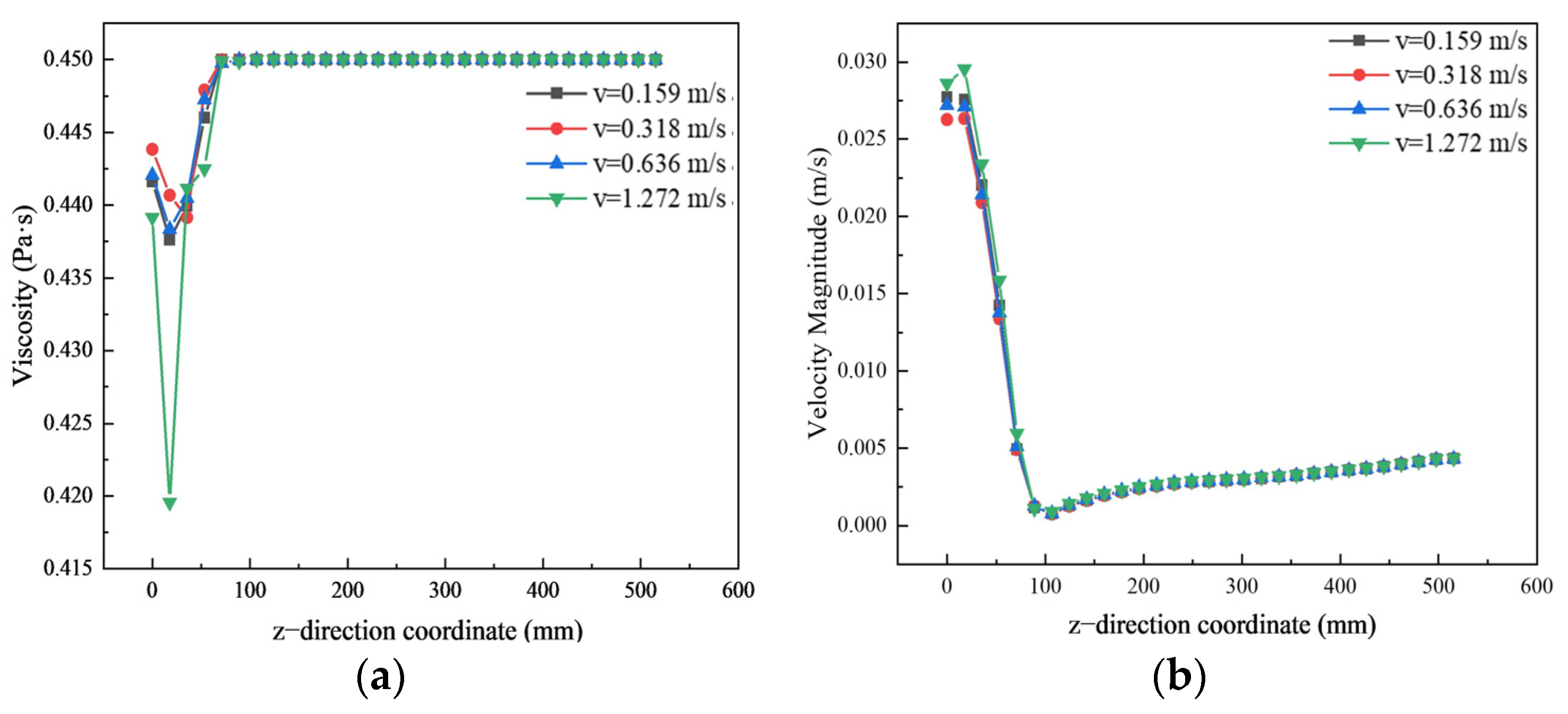
Figure 12a shows the viscosity change curve of gelatin solution in monitoring line b. When the z value exceeds 88 mm, the viscosity remains unchanged. However, when the z value is below 88 mm, the gelatin solution viscosity decreases due to an increase in the water volume fraction. Figure 12b shows the curve of velocity change along the positive direction of the z-axis at the outlet cross-section of monitoring line b. We can observe that along the positive direction of the z-axis, the velocity decreases first and then increases, and there is a minimum velocity when the z value is 106 mm.

3.3. Effect of Rotational Speed on Mixing Uniformity in a Helical Gear Pump Mixer

There is an important relationship between mixing uniformity and the speed of the helical gear pump mixer. As shown in

Table 4. Different speed conditions.

Case	Speed (0 to 9 s)	Speed (9 to 12 s)
a	8 rpm	50 rpm
b	20 rpm	50 rpm
c	30 rpm	50 rpm
d	40 rpm	50 rpm

, under the condition that the inlet speed remains unchanged at 0.318 m/s, we analyzed the volume fraction distribution of water in different outlet cross-sections of the helical gear pump mixer in a cycle at different rotational speeds.

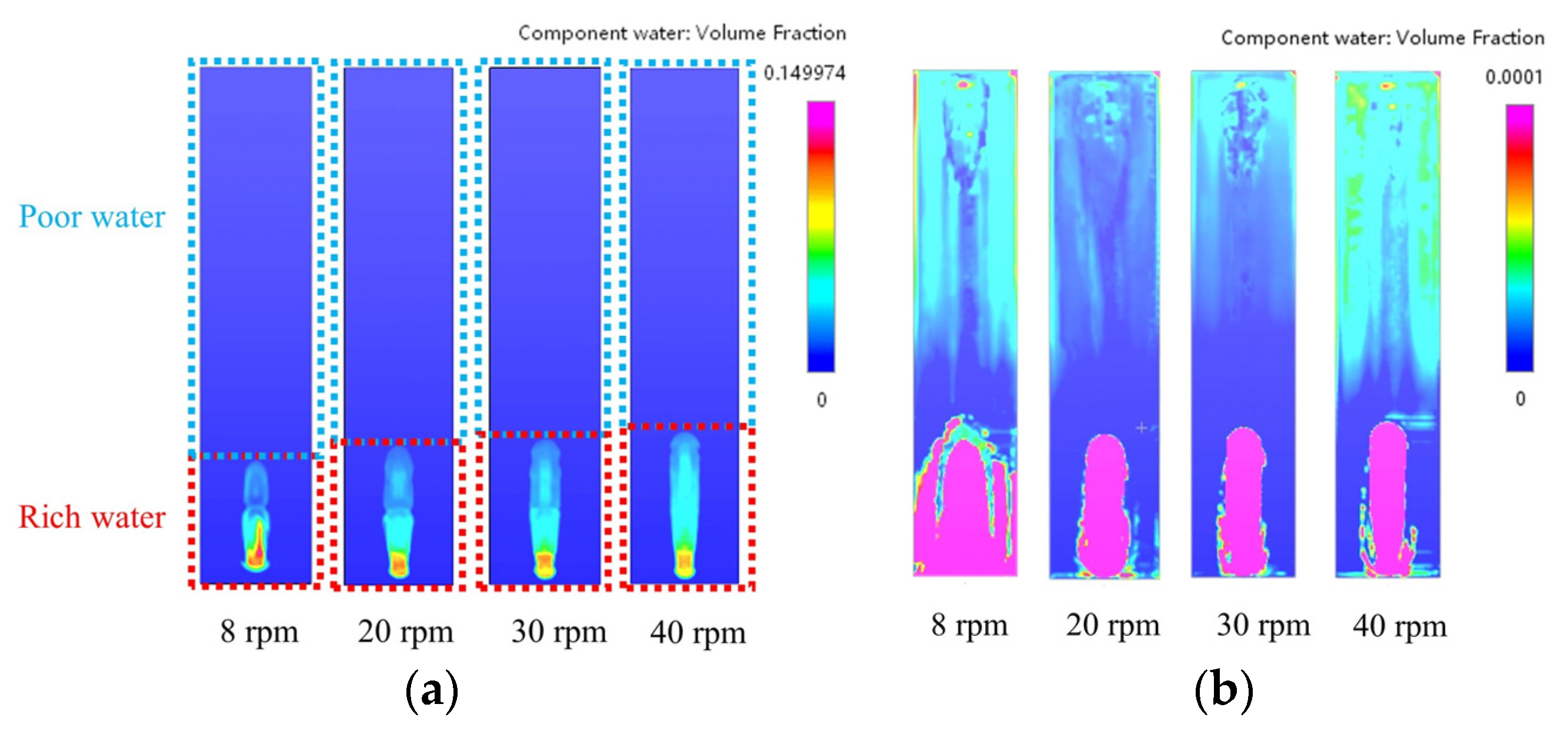
Figure 13a shows the volume fraction distribution of water at the outlet cross-section at different speeds (8 rpm, 20 rpm, 30 rpm, and 40 rpm). As the speed increases, the axial force and radial force of the gear increase, so that part of the water is transported faster to the back end, and the other part of the water enters the mixing tank area faster through the deflector. A water-rich region is formed at the front of the outlet cross-section. As shown in Figure 13b, as the rotational speed increases, the water in the mixing tank is transported more quickly to the back end, diluting the rich water area and causing the volume fraction of the water in the poor water region behind to increase significantly. This improves the uniformity of the gelatin solution with water in the mixing tank.

Figure 14 shows the water distribution at the x = 63.2 mm outlet cross-section under different rotational speeds. During a working cycle, as the rotational speed increases, the time for water to reach the back end of the mixing tank decreases, and the water is transported to the back faster. The volume fraction of water in the mixing tank gradually decreases along the positive direction of the z-axis. The water in the rich water zone is diluted, and the water in the poor water region is increased, which indicates that the water transport can be promoted at high rotational speed, and the mixing uniformity between gelatin solution and water can be improved.

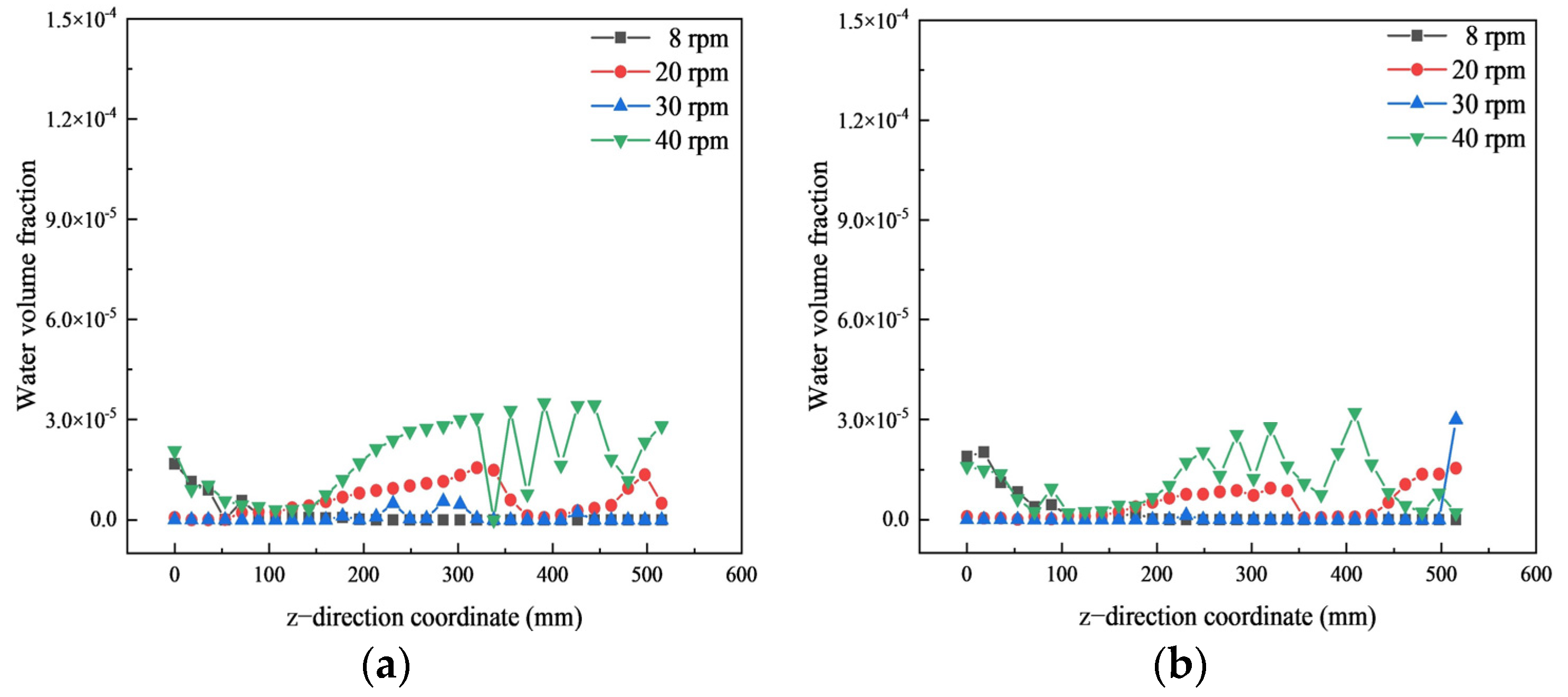
Figure 15a shows the distribution of the water volume fraction along the outlet cross-section monitoring line b along the z-axis. When the z value is less than 88 mm, the distribution of water is relatively dense, forming a water-rich area. Moving in the positive direction of the z-axis, the volume fraction of water shows a trend of increasing and then decreasing. The higher the rotational speed, the greater the volume fraction of water in the water-rich region. As shown in Figure 15b, when the z value is greater than 88 mm, the volume fraction of water at the end of the outlet cross-section is larger. At a speed of 40 rpm, the volume fraction of water is maximum at the end of the outlet cross-section. At high rotational speed, although the volume fraction of water in the rich water region increases, the water is also transported to the back of the mixing tank faster, which increases the volume fraction of water in the poor water region, and is conducive to improving the two-phase mixing uniformity in the poor water region.

Figure 16 shows the distribution of the water volume fraction at the outlet cross-section of monitoring lines a and c along the z-axis. With the increase in rotational speed, the average volume fraction of water in monitoring lines a and c is maximum at 40 rpm. In addition, the distribution trend of the water volume fraction in monitoring lines a and c is the same, which indicates that the distribution of water on the left and right sides is relatively uniform. Compared with monitoring line b in Figure 15a, we can see that the volume fraction of water along the x-axis presents a trend of being high in the middle and low on both sides.

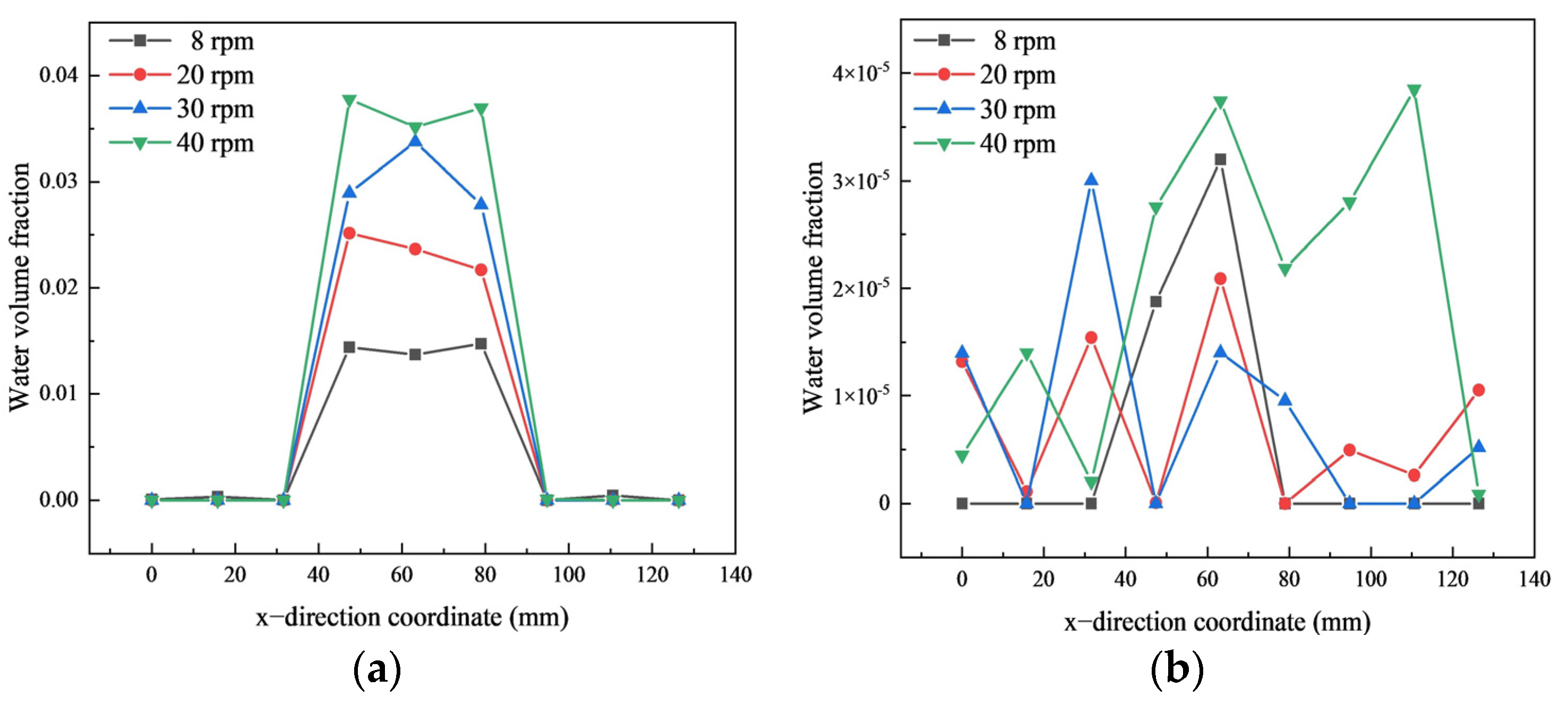
As shown in Figure 17a, in monitoring line d, the volume fraction of water at different rotational speeds reaches its maximum when x = 63.2 mm, and gradually decreases along both sides. When x = 63.2 mm, the volume fraction of water is minimum at 8 rpm and maximum at 40 rpm. As shown in Figure 17b, with the increase in rotational speed, the volume fraction of water fluctuates more, and the difference between the volume fraction of water on the left and right sides decreases. This indicates that the increase in speed promotes the water in the helical gear pump to reach the mixing tank faster, making the overall water volume fraction of the mixing tank increase uniformly.

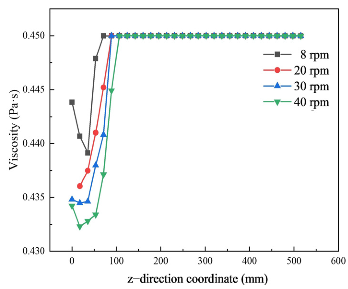
Figure 18 shows the viscosity change curve of gelatin solution in monitoring line b. With the increase in rotational speed, the viscosity of the water-rich region gradually decreases. Among them, it is worth noting that the z value of 88 mm is no longer the cut-off point for the change in gelatin solution viscosity. As the speed increases to 40 rpm, water is transported more quickly to the back end of the mixing tank, causing the cut-off point of the viscosity change in the gelatin solution to move backward from the z value of 88 mm to the z value of 106 mm.

4. Conclusions and Prospect

In this work, the numerical model of the helical gear pump mixer is established. The influence of different water inlet velocities (0.159 m/s, 0.318 m/s, 0.636 m/s, and 1.272 m/s) and different rotational speeds (8 rpm, 20 rpm, 30 rpm, and 40 rpm) on the mixing uniformity of the helical gear pump mixer was studied. The important conclusions drawn are as follows:

The flow field of the helical gear pump mixer was simulated by using Simerics MP+ commercial software. Compared with the traditional dynamic mesh, the software generates a structured mesh for the helical gear pump, which reduces the number of mesh elements and the calculation time. The volume fraction distribution of water in the outlet cross-section of a helical gear pump mixer filled with gelatin solution was obtained. The viscosity of monitoring line b was measured and compared with the simulation results to verify the reliability of the simulation.

In the actual work, due to the high volume fraction of water in the water-rich region, the viscosity changed greatly. However, the viscosity of the gelatin solution in the water-poor region remained stable, so the region with a z value greater than 88 mm should be selected in the actual operation process to avoid the diluting effect of the water-rich region on the viscosity of the gelatin solution.

The volume fraction of water in the water-rich region increases with increasing water inlet speed when the latter exceeds 0.318 m/s. At the same time, the volume fraction of water on the monitoring line showed a trend of being high in the middle and low on both sides along the x-axis, resulting in the distribution of water mainly concentrated in the middle of the outlet section and the edges on both sides, which was not conducive to the mixing of gelatin solution and water. When the v was 0.159 m/s, too low speed caused the water to mainly concentrate in the water-rich region. When the velocity was reduced from 1.272 m/s to 0.318 m/s, the maximum volume fraction of water in the water-rich region was reduced by 70.24%. In poor water regions, the maximum volume fraction of water increased by 9.25 times. Therefore, in the actual working process, the water inlet speed of 0.318 m/s should be used.

When the rotational speed increased from 8 rpm to 40 rpm, the water in the water-rich zone was delivered to the end faster. With the increase in time, the volume fraction of water in the rich water region was diluted and the volume fraction of water in the poor water region increased. Although the maximum volume fraction of the water-rich region increased by about 48% when the rotation speed was increased from 8 rpm to 40 rpm. However, the average volume fraction of water in the poor water region increased by 16.6 times on average at 40 rpm compared with 8 rpm. Therefore, increasing the speed is conducive to promoting the mixing uniformity of gelatin solution and water.

The simulation results show that the mixing uniformity of gelatin solution and water can be improved with a helical gear pump mixer at low water inlet speed and high rotation speed. On this basis, because the water distribution along the tooth width is high in the middle and low on both sides, the deflection plate and mixing tank can be further optimized to promote the generation of turbulence and further improve the mixing uniformity of the helical gear pump mixer. This study did not consider the effect of temperature on the mixing uniformity of gelatin solution and water, and the simulation period was short. Therefore, these factors should be incorporated into future surveys.

References

- Ransegnola, T.; Zhao, X.; Vacca, A. A comparison of helical and spur external gear machines for fluid power applications: Design and optimization. Mech. Mach. Theory 2019, 142, 103604. [Google Scholar] [CrossRef]
- Qi, F.; Dhar, S.; Nichani, V.H.; Srinivasan, C.; Wang, D.M.; Yang, L.; Bing, Z.; Yang, J.J. A CFD study of an electronic hydraulic power steering helical external gear pump: Model development, validation and application. SAE Int. J. Passeng. Cars-Mech. Syst. 2016, 9, 346–352. [Google Scholar] [CrossRef]
- Mo, S.; Zou, Z.; Feng, Z.; Dang, H.; Gao, H.; Cao, X. Research on lubrication characteristics of asymmetric helical gear based on CFD method. Lubr. Sci. 2020, 32, 309–320. [Google Scholar] [CrossRef]
- Saha, D.; Bhattacharya, S. Hydrocolloids as thickening and gelling agents in food: A critical review. J. Food Sci. Technol. 2010, 47, 587–597. [Google Scholar] [CrossRef]
- Toh, M.; Gondoh, T.; Mori, T.; Mishima, M. Mixing characteristics of an internal mixer: Uniformity of mixed rubber. J. Appl. Polym. Sci. 2005, 95, 166–172. [Google Scholar] [CrossRef]
- Liu, Y.Z.; Kim, B.J.; Sung, H.J. Two-fluid mixing in a microchannel. Int. J. Heat Fluid Flow 2004, 25, 986–995. [Google Scholar] [CrossRef]
- Florian-Algarin, M.; Méndez, R. Blend uniformity and powder phenomena inside the continuous tumble mixer using DEM simulations. AIChE J. 2015, 61, 792–801. [Google Scholar] [CrossRef]
- Mucchi, E.; Dalpiaz, G. Elasto-dynamic analysis of a gear pump–Part III: Experimental validation procedure and model extension to helical gears. Mech. Syst. Signal Process. 2015, 50, 174–192. [Google Scholar] [CrossRef]
- Diab, Y.; Ville, F.; Houjoh, H.; Sainsot, P.; Velex, P. Experimental and numerical investigations on the air-pumping phenomenon in high-speed spur and helical gears. Proc. Inst. Mech. Eng. Part C J. Mech. Eng. Sci. 2005, 219, 785–800. [Google Scholar] [CrossRef]
- Huang, K.; Chen, C.; Chang, Y. Geometric displacement optimization of external helical gear pumps. Proc. Inst. Mech. Eng. Part C J. Mech. Eng. Sci. 2009, 223, 2191–2199. [Google Scholar] [CrossRef]
- Zhao, X.; Vacca, A. Analysis of continuous-contact helical gear pumps through numerical modeling and experimental validation. Mech. Syst. Signal Process. 2018, 109, 352–378. [Google Scholar] [CrossRef]
- Frosina, E.; Senatore, A.; Rigosi, M. Study of a high-pressure external gear pump with a computational fluid dynamic modeling approach. Energies 2017, 10, 1113. [Google Scholar] [CrossRef]
- Castilla, R.; Gamez-Montero, P.; Ertürk, N.; Vernet, A.; Coussirat, M.; Codina, E. Numerical simulation of turbulent flow in the suction chamber of a gearpump using deforming mesh and mesh replacement. Int. J. Mech. Sci. 2010, 52, 1334–1342. [Google Scholar] [CrossRef]
- Ghazanfarian, J.; Ghanbari, D. Computational fluid dynamics investigation of turbulent flow inside a rotary double external gear pump. J. Fluid. Eng. 2015, 137, 21101. [Google Scholar] [CrossRef]
- Li, L.; Versteeg, H.K.; Hargrave, G.K.; Potter, T.; Halse, C. Numerical investigation on fluid flow of gear lubrication. SAE Int. J. Fuels Lubr. 2009, 1, 1056–1062. [Google Scholar] [CrossRef]
- Ji, Z.; Stanic, M.; Hartono, E.A.; Chernoray, V. Numerical simulations of oil flow inside a gearbox by Smoothed Particle Hydrodynamics (SPH) method. Tribol. Int. 2018, 127, 47–58. [Google Scholar] [CrossRef]
- Mithun, M.-G.; Koukouvinis, P.; Karathanassis, I.K.; Gavaises, M. Numerical simulation of three-phase flow in an external gear pump using immersed boundary approach. Appl. Math. Model. 2019, 72, 682–699. [Google Scholar] [CrossRef]
- Li, J.; Qian, X.; Liu, C. Comparative study of different moving mesh strategies for investigating oil flow inside a gearbox. Int J Numer. Methods Heat Fluid Flow 2022, 32, 3504–3525. [Google Scholar] [CrossRef]
- Zhao, X.; Vacca, A. Multi-domain simulation and dynamic analysis of the 3D loading and micromotion of continuous-contact helical gear pumps. Mech. Syst. Signal Process. 2022, 163, 108116. [Google Scholar] [CrossRef]
- Salawu, E.Y.; Ajayi, O.O.; Okeniyi, J.O.; Inegbenebor, A.O.; Afolalu, S.; Ongbali, S.; Banjo, S. On the prediction of power loss in helical gearbox via simulation approach. Clean. Eng. Technol. 2021, 3, 100128. [Google Scholar] [CrossRef]
- Zhou, C.; Jiang, X.; Su, J.; Liu, Y.; Hou, S. Injection lubrication for high-speed helical gears using the overset mesh method and experimental verification. Tribol. Int. 2022, 173, 107642. [Google Scholar] [CrossRef]
- Heisler, A.S.; Moskwa, J.J.; Fronczak, F.J. Simulated helical gear pump analysis using a new CFD approach. In Proceedings of the Fluids Engineering Division Summer Meeting, Vail, CO, USA, 2–6 August 2009. [Google Scholar] [CrossRef]
- Simerics Inc. Simerics MP+’s User Manual—V 5.2.15; Simerics: Bellevue, WA, USA, 2022. [Google Scholar]
- Hirt, C.W.; Nichols, B.D. Volume of fluid (VOF) method for the dynamics of free boundaries. J. Comput. Phys. 1981, 39, 201–225. [Google Scholar] [CrossRef]
- Scardovelli, R.; Zaleski, S. Direct numerical simulation of free-surface and interfacial flow. Annu. Rev. Fluid Mech. 1999, 31, 567–603. [Google Scholar] [CrossRef]
- Zhang, X.; Zhang, B.; Cao, J.; Su, L.; Li, K. Numerical investigation on the performance and vapor injection process of a scroll compressor with different injection features. Appl. Therm. Eng. 2022, 217, 119061. [Google Scholar] [CrossRef]
Figure 1.
Helical gear pump mixer computational domain. (a) Helical gear pump mixer main view. (b) Helical gear pump left view. (c) Helical gear pump mixer main view, partially enlarged. (d) Helical gear pump top view.
Figure 2.
Grid division and partial amplification. (a) Helical gear pump mixer main view. (b) Helical gear pump left view. Note: Red circles indicate locally enlarged areas. The red arrow points to a partially enlarged image.
Figure 3.
Helical gear pump mixer operating condition diagram. (a) Water inlet velocity variation within a single working cycle. (b) Variation in gear speed within a single working cycle.
Figure 4.
Boundary conditions. (a) Helical gear pump mixer main view. (b) Helical gear pump mixer elevation view. Note: 1–7 represent gelatin solution inlet 1 to gelatin solution inlet 7.
Figure 5.
Monitoring point setting. (a) Outlet cross-section of the numerical model. (b) Actual outlet cross-section.
Figure 6.
Experimental verification. (a) Outlet mass flux. (b) Monitor viscosity of the gelatin solution at the outlet cross-section of line b.
Figure 7.
Volume fraction distribution of water. (a) Volume fraction cloud image at different water inlet velocities. (b) Local amplification of volume fraction.
Figure 8.
The volume fraction distribution of water in the x = 63.2 mm section at different water inlet velocities.
Figure 9.
Volume fraction distribution of water at outlet section. (
a) Volume fraction distribution of water in monitoring line b. (
b) Monitor line b local amplification. Note: The yellow line shows the dividing line between rich and poor water regions, the blue dashed box shows the area of partial enlargement in
Figure 9b.
Figure 10.
Distribution of water volume fraction in outlet cross-section at different inlet velocities. (a) Volume fraction distribution of water in monitoring line a. (b) Volume fraction distribution of water in monitoring line c. Note: The yellow line shows the dividing line between rich and poor water regions.
Figure 11.
Volume fraction distribution of water at outlet section. (a) Volume fraction distribution of water in monitoring line d. (b) Volume fraction distribution of water in monitoring line f.
Figure 12.
Volume fraction distribution of water at outlet section. (a) Viscosity of gelatin solution at different inlet velocities along the z-axis. (b) Velocity of gelatin solution at different inlet velocities along the z-axis.
Figure 13.
Volume fraction distribution of water. (a) Volume fraction cloud image at different rotational speeds. (b) Local amplification of volume fraction.
Figure 14.
The volume fraction distribution of water in the x = 63.2 mm section at different rotational speeds.
Figure 15.
b) Local amplification. Note: The yellow line shows the dividing line between rich and poor water regions, the blue dashed box shows the area of partial enlargement in
Figure 15b.
Figure 16.
Volume fraction distribution of water at different rotational speeds. (a) Volume fraction distribution of water in monitoring line a. (b) Volume fraction distribution of water in monitoring line c.
Figure 17.
Volume fraction distribution of water at outlet section. (a) Volume fraction distribution of water in the d monitoring line. (b) The f monitoring line water volume fraction distribution.
Figure 18.
Change curve of viscosity along the tooth width direction at different rotational speeds.