Effects of Topological Properties with Local Variable Apertures on Solute Transport through Three-Dimensional Discrete Fracture Networks

Abstract

In this study, the effects of topological properties with local variable apertures on fluid flow and solute transport through three-dimensional (3D) discrete fracture networks (DFNs) were investigated. A series of 3D DFNs with different fracture density, length, and aperture distribution were generated. The fluid flow and solute transport through the models were simulated by combining the MATLAB code and COMSOL Multiphysics. The effects of network topology and aperture heterogeneity on fluid flow and transport process were analyzed. The results show that the fluid flow and solute transport exhibit a strong channeling effect even in the DFNs with identical aperture, in which the areas of fast and slow migration fit well with the high- and low-flow regions, respectively. More obvious preferential paths of flow and migration are observed in individual fractures for the DFN with heterogeneous aperture than the model with identical aperture. Increasing the fracture length exponent reduces the available flow and transport paths for sparse fracture networks but does not significantly change the flow and transport channels for dense fracture networks. The breakthrough curves (BTCs) shift towards the right and slightly lag behind as the fracture density decreases or the aperture heterogeneity increases. The advection–diffusion equation (ADE) model cannot properly capture the evolution of BTCs for 3D DFNs, especially the long tails of BTCs. Compared to the ADE model, the mobile-immobile model (MIM) model separating the liquid phase into flowing and stagnate regions is proven to better fit the BTCs of 3D DFNs with heterogeneous aperture.

1. Introduction

Modeling of flow and transport processes through rock fractures is critical for both environmental and engineering applications, such as nuclear waste disposal [1,2], CO₂ geological storage [3,4], and geothermal energy development [5,6]. Since the permeability of fractures is typically orders of magnitude larger than that of the rock matrix, well connected fractures may act as primary conduits for the migration of fluids and hazardous materials [7,8,9]. Accurate characterization of coupled flow and transport mechanism in rock fracture networks is essential for the overall understanding of the fractured reservoir behavior.

Continuous [10,11,12,13,14] and discrete methods [15,16,17,18,19,20] have been proposed to model the discontinuous fractured rocks. For the dense fractures over a large domain size, the continuous method is effective and convenient by characterizing the contribution of fractures as equivalent parameters. On the other hand, when the fractures are sparsely distributed and detailed heterogeneities are of interest, the discrete method is more suitable since it can explicitly represent the geometrical structure of individual fractures. The discrete fracture network (DFN) modeling approach characterizes the fracture as segment lines in two dimension or planar polygons in three dimensions, which can be denoted as 2D DFN and 3D DFN, respectively [21,22,23]. Previous investigations have demonstrated that 2D DFNs, which can be regarded as the cut planes from 3D DFNs, cannot capture the 3D structure of individual fractures, and thus underestimate the connectivity of fracture networks. In the present study, the 3D DFN modeling approach will be applied to focus on the flow and transport within discrete fractures in detail.

Since natural fractures inside the rock masses are complex and invisible, the stochastic approach has been applied in DFNs by characterizing the geometrical properties of fractures (e.g., fracture size, location, density, orientation, and aperture) in a stochastic framework. This uncertainty requires a well understanding of how the distribution of fracture properties affect the network-scale hydraulic and transport behaviors. Maillot et al. [24] analyzed the influence of spatial structure of fractures on the connectivity and permeability of DFNs. They concluded that the kinematical DFNs where fractures result from a growth process have a 1.5–10 times larger permeability compared to the randomly distributed DFNs. Frampton et al. [25] analyzed the influence of variable apertures represented by different texture types on the flow and transport in 3D DFNs. They concluded that internal variability textures of fractures can either increase or decrease solute travel times depending on the relative connectivity of networks. Kang et al. [26] captured the anomalous transport in 3D DFNs by changing the injection mode and aperture distribution between fractures. They demonstrated that the velocity distribution is determined by considering the aperture heterogeneity and injection mode controls of the effective transport through 3D DFNs. The heterogeneity of 3D DFNs originates from both fracture-scale variabilities such as surface roughness and aperture, and network-scale topological properties such as fracture density and fracture length distribution [25,26,27,28]. The effect of combined two scales of heterogeneity on the solute transport in 3D DFNs has not been thoroughly understood, and improving the understanding of such effects is significant for many applications to predict the first arrival and long residence time of particles in DFNs.

Solute transport through rock fractures is traditionally modeled using Fick’s law where the breakthrough curves (BTCs) can be captured by the advection dispersion equation (ADE) [29]. However, many laboratory tests [30,31] and numerical simulations [32,33,34,35] of solute transport through single rough-walled fractures indicate that the classical ADE fails to describe the early arrival and long tailing of the BTCs, which is denoted as non-Fickian behavior. Several approaches such as the mobile-immobile model (MIM) [36], continuous time random walk (CTRW) [37], and stratified model [38] have been developed to explain this phenomenon of non-Fickian behavior. Bauget and Fourar [39] confirmed that the CTRW model is able to model the long time tailing of BTCs observed in the tracer experiment on a single fracture. Dou et al. [40] regarded the roughness-induced eddies as an immobile region and obtained a better fitness of BTCs by the MIM model compared to the ADE model. The non-Fickian transport behavior has also been frequently observed in the DFNs that have smooth even surface [41]. Cherubini et al. [42] compared the performances of the explicit network model (ENM) and the MIM model to fit the anomalous BTCs for 2D DFNs. They found that although the fitting results of ENM are better than that of MIM, the latter can also describe the BTCs quite well. However, the reliability of the analytical models to describe the non-Fickian transport process in 3D DFNs is still not clear.

The goal of this study is to investigate the effects of topological properties with local variable apertures on solute transport through 3D DFNs and examine the reliability of analytical models to describe the transport process in fractured rock masses. For this, a number of 3D DFNs that have increasing fracture density and fracture length were established, in which the aperture of the individual fracture follows heterogeneous distributions. Fluid flow and solute transport were simulated by combining the MATLAB code and COMSOL Multiphysics. The effects of network topology and aperture heterogeneity on fluid flow and transport process were analyzed. The inverse ADE and MIM models for BTCs were estimated.

2. Methodology

2.1. Generation of 3D DFNs

The scale of rock fractures usually ranges from millimeter to kilometer [43]. The geometrical properties of fractures, such as location, length, density, orientation, and aperture, are often described in terms of statistical distributions. In this study, rock fractures are represented by circular disks having uniformly distributed orientation and location. Under such simplifications, the geometrical features of fracture length, density, and aperture control the overall flow and transport behaviors through fracture networks. Many field investigations have found that the following power law function can be used to model the distribution of fracture length [44]:

$$\mathrm{n}\left(l\right)=\mathsf{\alpha }·l^{-a}$$

(1)

where l represents the fracture length, α is the proportionality coefficient representing the total amount of fractures by the range of fracture length, and a is the power low exponent controlling the relative proportion of longer and shorter fractures in DFNs. Field observation from outcrops indicates that the value of a of natural rock fractures generally ranges within 2.0~4.5 [45]. A larger magnitude of a will result in a series of fractures having smaller fracture length, and vice versa. The parameter P₃₂, defined as the total fracture surface per unit volume, was utilized to measure the fracture density. To examine the influence of topological properties of fracture networks on flow and transport behaviors, a number of 3D DFNs of size 10 m × 10 m × 10 m were established, for which three increasing fracture densities of P₃₂ = 0.45, 0.65, 0.85, and 1.05 m²/m³, and two different fracture length distributions of a = 2.0 and 4.5 were considered. The generated 3D DFNs with different P₃₂ and a are depicted in Figure 1.

The fracture aperture of the natural rock fracture is usually heterogeneously distributed due to its two rough surface walls [46,47]. Such a heterogeneous aperture field can be modeled according to the truncated Gaussian distribution, written as [48]:

$$\mathrm{f}\left(b\right)=\left\{\begin{array}{c}\frac{1}{\sigma \sqrt{2\pi }}{e}^{-\frac{{\left(b-b_m\right)}^2}{2{\sigma }^2}} \mathrm{i}\mathrm{f} b\ge 0\\ 0 \mathrm{i}\mathrm{f} b<0\end{array}\right.$$

(2)

where b is the fracture aperture, and b_m and σ represent the mean and standard deviation of aperture distribution, respectively. The estimated negative value in Equation (2) is assigned to be zero, representing the contact between the upper and lower surfaces of a fracture. The applicability of truncated Gaussian distribution to characterize the aperture distribution within rough-walled fractures has been clarified by laboratory measurements of natural rock fractures and this distribution has been frequently used in previous fracture aperture modeling [45,49,50]. In order to account for the aperture heterogeneity, four increasing σ = 0.0, 1.0, 2.0, and 3.0 mm with the same b_m = 1.72 mm were considered, resulting in a series of 3D DFNs having a same network topology but different aperture distributions. In total, 32 DFNs with different fracture density, fracture length, and aperture distribution were generated to investigate the effects of topological properties with local variable apertures on solute transport. It should be noted that the fracture topological properties are not directly identical to the actual situation, but their distributions, such as fracture length characterized by power-law distribution and fracture aperture characterized by truncated Gaussian distribution, are identical to the observations of geological fractured media and have been widely used in the previous DFN modeling [44,45,51,52]. Figure 2 displays the frequency of the four aperture distributions. For each aperture distribution, a stream of random numbers are used to generate different aperture patterns between fractures in the 3D DFNs.

2.2. Fluid Flow

The Navier–Stokes equation written as follows is utilized to model the fluid flow through fractured rocks [53]:

$$\rho \left[\frac{\partial \mathbf{u}}{\partial t}+\left(\mathbf{u}·\nabla \right)\mathbf{u}\right]=-\nabla P+\nabla ·\mathbf{T}+\rho \mathbf{f}$$

(3)

where u is the flow velocity, P is the fluid pressure, ρ is the fluid density, T is the shear stress tensor, and f is the acceleration of gravity, whereas the exact solution of Navier–Stokes equation is usually difficult to achieve due to the nonlinearity terms (u $·\mathbf{\nabla }$)u, especially for cases with complex fracture networks. When the pressure gradient of flow is small enough to reach a laminar flow, the nonlinear terms (u $·\mathbf{\nabla }$)u can be ignored and the Navier–Stoke equations is reduced to the Stokes equation. By integrating the Stokes equation over the fracture aperture, the following equation is obtained to estimate the volumetric flow rate of fracture:

$$Q=-T\nabla P$$

(4)

where Q represents the volumetric flow rate, and T denotes the transmissivity, which can be related with aperture as [26,54]:

$$T=\frac{b^3}{12\mu }$$

(5)

where μ represents the dynamic fluid viscosity. The local flux which is equal to the integral of the flow velocity along fracture aperture is conservative, which yields the following equation:

$$\nabla ·Q=0$$

(6)

Substituting Equations (4) and (5) into Equation (6), the following equation known as the Reynolds equation can be obtained:

$$\nabla ·\left(b^3\nabla P\right)=0$$

(7)

To account for the aperture heterogeneity in each single fracture, the magnitude of b in Equation (7) is spatially assigned according to Equation (2). For the overall flow in fracture networks, Equation (7) modeled in individual fracture is complemented with the continuous flux and hydraulic head along fracture intersections. This requires a conforming triangulation at intersections that the nodes on trace lines are consistent with the discretization of each intersecting fracture and the element edges of trace lines divided by these nodes are shared by intersecting fractures, as shown in Figure 3a. As displayed in Figure 3b, a Dirichlet boundary condition consisting of two fixed hydraulic heads at the left and right faces of the cube, and a Neumann boundary condition consisting of impervious boundaries at other flour orthogonal faces of the model, are considered in the flow simulation. The fluid flow process is solved using the finite element method and is implemented by combining the MATLAB code and COMSOL Multiphysics. Taking the DFN model with P₃₂ = 1.05 m²/m³ and a = 4.5 as an example, the total amount of triangular elements was 592,119 in which the maximum and minimum element size were 0.1991 m and 4.3533 × 10⁻⁴ m, respectively. To perform the mesh-independent analysis, two models with a total amount of element increasing from 592,119 to 1,425,178 were generated. The results show that the discrepancy of the simulated flow rates between those two models under the same hydraulic gradient is less than 0.2%, which indicates that the 592,119 elements were sufficient to achieve a stable simulation. The estimated flow field was then coupled to the simulation of solute transport.

2.3. Solute Transport

The following advection–diffusion equation (ADE) is used to model the conservative solute transport through rock fractures [55]:

$$\frac{\partial c}{\partial t}=-\mathbf{u}·\nabla c+\nabla ·\left(\mathbf{D}\nabla c\right)$$

(8)

where c represents the volumetric concentration and D represents the dispersion coefficient tensor. When the flow velocity u is replaced by the mean velocity V, the BTCs can be analyzed based on the analytic solution of the ADE, written as [56]:

$$c\left(x,t\right)=\frac{C_0}{2}\left[\mathrm{e}\mathrm{r}\mathrm{f}\mathrm{c}\left(\frac{x-Vt}{2\sqrt{D_{L}t}}\right)+\mathrm{e}\mathrm{x}\mathrm{p}\left(\frac{Vx}{D_L}\right)\mathrm{e}\mathrm{r}\mathrm{f}\mathrm{c}\left(\frac{x+Vt}{2\sqrt{D_{L}t}}\right)\right]$$

(9)

where c₀ is the inlet concentration and D_L is the fitted dispersion coefficient. Equation (9) is derived based on the smooth fracture with constant aperture and uniform flow velocity. When applying to the rough-walled fracture with heterogeneous apertures, the D_L is taken as an adjustable parameter to fit the BTCs. As a result, the D_L estimated based on Equation (9) cannot predict the non-Fickian behaviors of transport. The MIM model separating the liquid phase into flowing and stagnate regions has been proven to better explain the non-Fickian feature of the transport [57]. The MIM model can be written as:

$${\theta }_m\frac{\partial c_m}{\partial t}={\theta }_m{D}_m\frac{{\partial }^2{c}_m}{\partial x^2}-V{\theta }_m\frac{\partial c_m}{\partial x}-\delta \left(c_m-c_{im}\right)$$

(10)

$${\theta }_{im}\frac{\partial c_{im}}{\partial t}=\omega \left(c_m-c_{im}\right)$$

(11)

where c_m and c_im represent the concentration in the mobile and immobile domain, respectively; D_m represents the dispersion coefficient, $\omega$ is the dimensionless mass transfer coefficient, θ_m and θ_im denote the water contents in the mobile and immobile regions, respectively, and θ_m + θ_im = 1 for the saturated flow in fractures. A dimensionless quantity β = θ_m/(θ_m + θ_im) is defined to represent the fraction of mobile water. Due to the complex geometry of fracture intersection and aperture heterogeneity, fluid flows in 3D DFNs along some preferred pathways, accompanied with regions of extremely low- and high-flow rate, respectively [21]. In this study, these extremely low-flow rate regions are viewed as the immobile regions to implement the MIM model. As shown in Figure 3b, the solute concentration in the fractures was set to zero as the initial condition with a dimensionless inlet concentration c = c₀ = 1.0 imposed on the inflow boundary. The effluent solute mass can be calculated by integrating the fluid flux and concentration along the outlet boundary. The BTCs is estimated to be the ratio of effluent solute mass to fluid mass, written as:

$$c_f=\frac{{\displaystyle {\int }_{\Gamma }ub\cdot cds}}{{\displaystyle {\int }_{\Gamma }ubds}}$$

(12)

where Γ denotes the outlet boundary. In Equation (12), the concentration at the outlet boundary is weighted by the flow flux. Furthermore, the BTCs are normalized by the injection concentration, which is:

$$c^{\prime }=\frac{c_f}{c_0}$$

(13)

where c₀ is the injection concentration, and c’ is the dimensionless concentration.

2.4. Inverse Parameters from BTCs

The ADE model is strictly derived from the single fracture with smooth surface and uniform flow velocity [58]. When applying the ADE model to the DFNs with heterogeneous apertures, very poor agreement will be obtained if using the mean flow velocity estimated from the simulation and setting the D_L as the one adjustable parameter. As a result, both V and D_L in the ADE model are regarded as adjustable parameters, which has also been frequently used in the previous study on the solute transport in rough-walled fractures [59,60]. For the MIM model, the initial values of V and D_m are set equal to that estimated from the ADE model, which will improve the convergence of the inverse estimation [40]. The parameters in the ADE or MIM model are estimated based on the simulated BTCs using the CXTFIT code in Excel developed by [61]. The global error E_m is used to quantify the goodness of fit of results, written as [40]:

$$E_m=\sqrt{{\sum }_i^N{\left(c_{fit,i}-c_s\right)}^2/N}$$

(14)

where c_fit,i (i = 1, 2, 3, …, N) is the concentration in the fitted BTCs using the ADE or MIM model, c_s is the concentration estimated based on the direct simulation, N represents total number of data in the BTCs, m denotes the ADE or MIM model, and the E_m hereafter is denoted as E_ADE and E_MIM, representing the estimated results from the ADE model and the MIM model, respectively.

3. Results

3.1. Effects of Network Topology

As illustrated in Figure 1, the geometrical features that control the topology of the networks are the fracture density and fracture length exponent a. Fluid flow and solute transport through DFNs with different P₃₂ = 0.45, 0.65, 0.85, and 1.05 m²/m³, and a = 2.0 and 4.5 are simulated. Without loss of generality, Figure 4a–d only show the results in DFNs with a = 2.0 and σ = 0 mm, in which the influences of fracture density on flow channel can be observed. The color intensity in Figure 4a–d represents the ratio of flow rate at each point to the total flow, implying the contribution of local element to the total flow. Despite the fact that all the fractures in the DFNs have an identical aperture, their generated preferential flow paths with the main flow channels are concentrated in a few fractures. This phenomenon of channeling flow results from the arrangement of fractures in the networks, i.e., the connectivity of DFNs. For the DFNs with a smaller P₃₂, only a few fractures connecting the inlet and outlet boundaries allow the fluid to flow through. As P₃₂ increases, the number of connected fractures increases, thereby providing more potential flow pathways.

The evolution of solute concentration distributed in these flow channels are displayed in Figure 4e–h at different timescales: after an intermediate time of t = 1000 s (Figure 4e–h), and t = 3000 s (Figure 4i–l) when the solute has migrated to the outlet boundary. It is obvious that the solute migrates following the main flow channels towards the outlet boundary, in which the areas of fast- and slow-migration fit well with the high- and low-flow regions in Figure 4a–c, respectively. Figure 5 indicates the evolutions of BTCs with fracture densities for 3D DFNs possessing different aperture distributions. It can be seen that the arrival time of DFNs with denser fractures is earlier than that with sparse fractures due to more available flow paths, which is more distinct in the DFNs of larger σ. The BTCs slightly lag behind as σ increases, because the low velocity in the small-aperture regions hinder the flow and solute migration, which will be further illustrated in the following section.

Figure 6 displays the flow rate and concentration field in the 3D DFNs with different fracture densities when a = 4.5 and σ = 0 mm. Comparison of Figure 5 and Figure 6 shows that the available flow paths in the DFNs decrease as a increases, resulting in the delay of solute migration. This phenomenon is more distinct for the model having a small fracture density of P₃₂ = 0.45 m²/m³. This is because decreasing the fracture length would significantly reduce the network connectivity when the density of DFNs is relatively small, thereby hindering the fluid flow and solute transport. On the contrary, as fracture density increases, decreasing the fracture length does not cause drastic change in the network connectivity, but rather adds smaller fractures to the existing connected pathways. This tendency can also be obtained by comparing the BTCs of DFNs with a = 2.0 and a = 4.5 shown in Figure 7, in which a remarkable delay in BTCs for the model with a = 2.0 and P₃₂ = 0.45 m²/m³ is observed. The discrepancy in BTCs between the models with a = 2.0 and a = 4.5 significantly decreases as the P₃₂ increases to 1.05 m²/m³ as shown in Figure 7d.

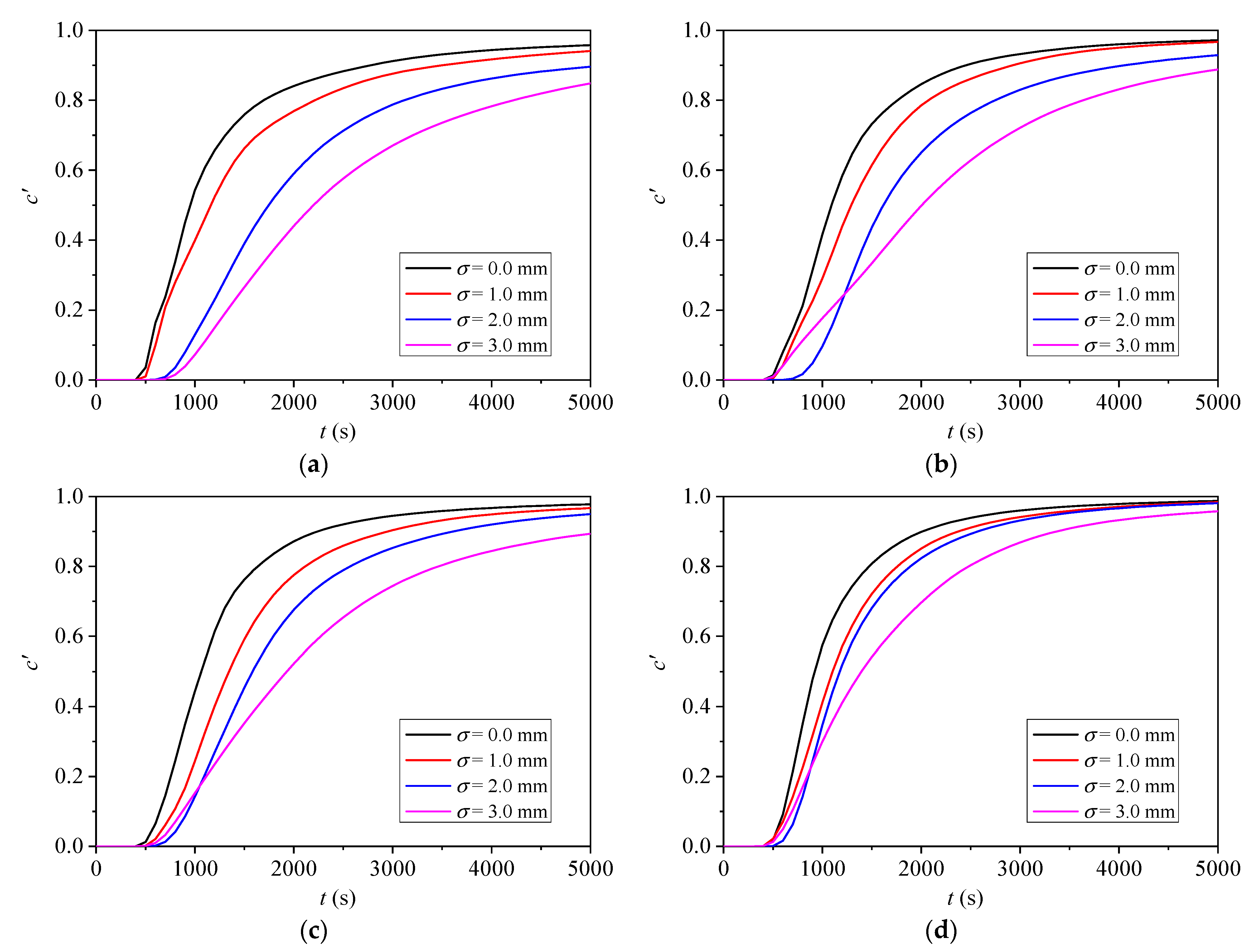
3.2. Effects of Aperture Heterogeneity

To explore the influence of aperture heterogeneity on the fluid flow and solute transport, four different aperture distributions with increasing standard deviation of σ = 0.0, 1.0, 2.0, and 3.0 mm are assigned to each individual fracture in the DFNs. Without loss of generality, Figure 8a–d only display different aperture patterns in DFNs with a = 2.0 and P₃₂ = 0.65 m²/m³. Note that all the models have the same mean aperture of b_m = 1.72 mm. It is obvious that as σ increases, the aperture heterogeneity increases, resulting in a more pronounced phenomenon of channeling flow as shown in Figure 8e–h. These flow pathways are located primarily within the channels of large aperture and bypass the obstacles of low aperture. The spatial evolutions of concentration fields are shown in Figure 8i–p, and are found to be sensitive to the flow channels. The solute migrates faster in the high-flow channels than in the low-flow regions, clearly showing that the concentration field forms advection channels along the preferential flow paths. This phenomenon of transport channels is more pronounced in the DFNs possessing a larger σ.

Figure 9 displays the evolutions of BTCs with fracture aperture distribution for 3D DFNs having different fracture densities. For all cases with different fracture density, as σ increases, the BTCs shift towards the right with long tails and need increasing time for the solute to reach the outlet boundary. This is because when the aperture heterogeneity increases, more solute is trapped in the low-flow regions with small aperture. With increasing P₃₂, the deviation of BTCs between σ = 0.0 and 3.0 mm decreases, which indicates a limited reduction effect in aperture heterogeneity on the solute transport. On the other hand, as P₃₂ increases, an obvious early arrival of BTCs is observed for the model with σ = 3.0 mm. This is due to the fact that the increasing aperture heterogeneity promotes some solute migration fast along the preferential paths, allowing for the early arrival of some solute to the outlet boundary, which further illustrates that aperture heterogeneity plays a significant role in the solute migration process. For a small fracture density, the probability of generating slow-migration areas induced by low aperture barriers is increased. As fracture density increases, more connecting fractures provide additional alternatives, allowing the solute to bypass the low aperture barriers and enhancing the solute migration. As a result, the change in geometrical configuration induced by fracture density weakens the influences of aperture heterogeneity on the solute migration.

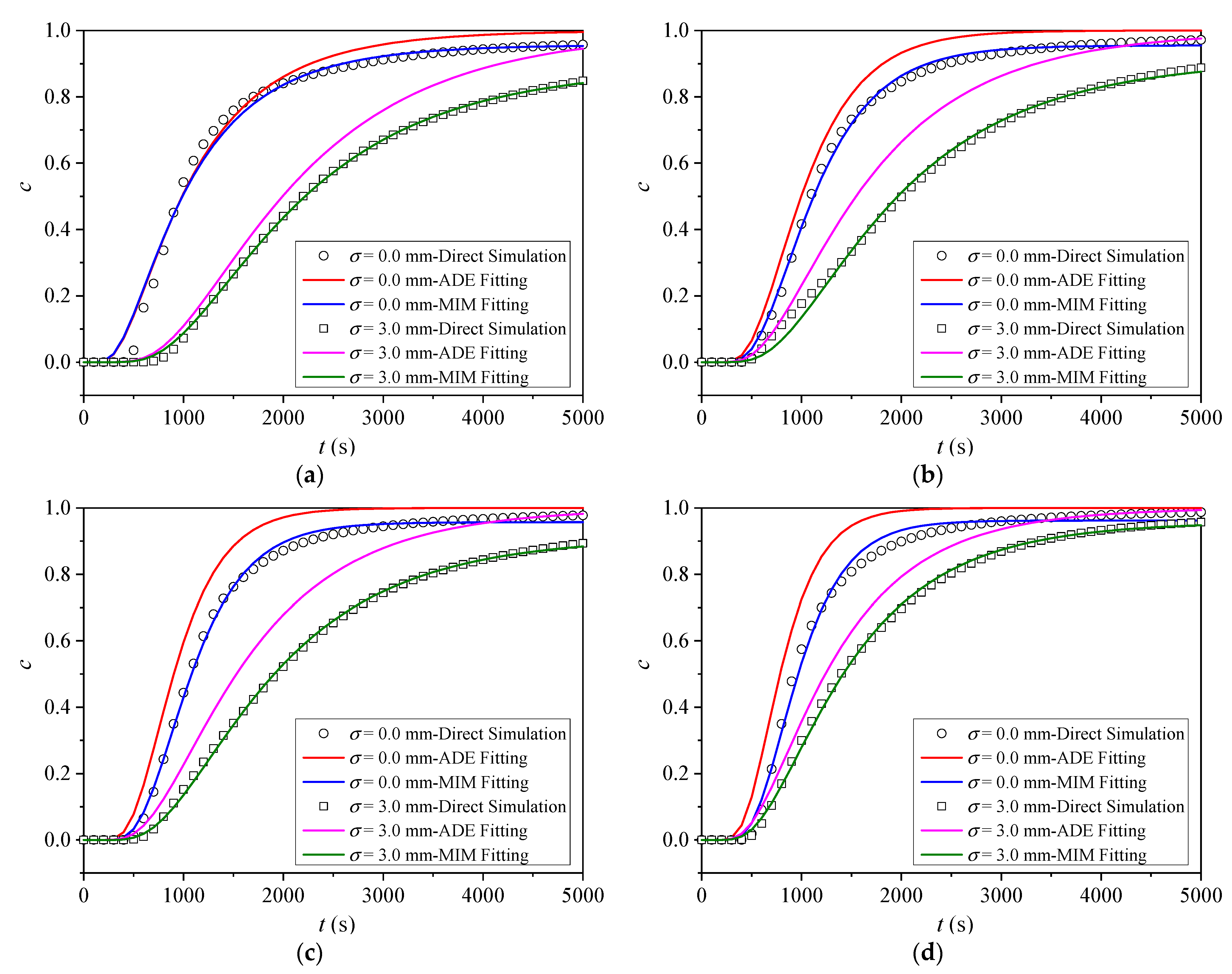
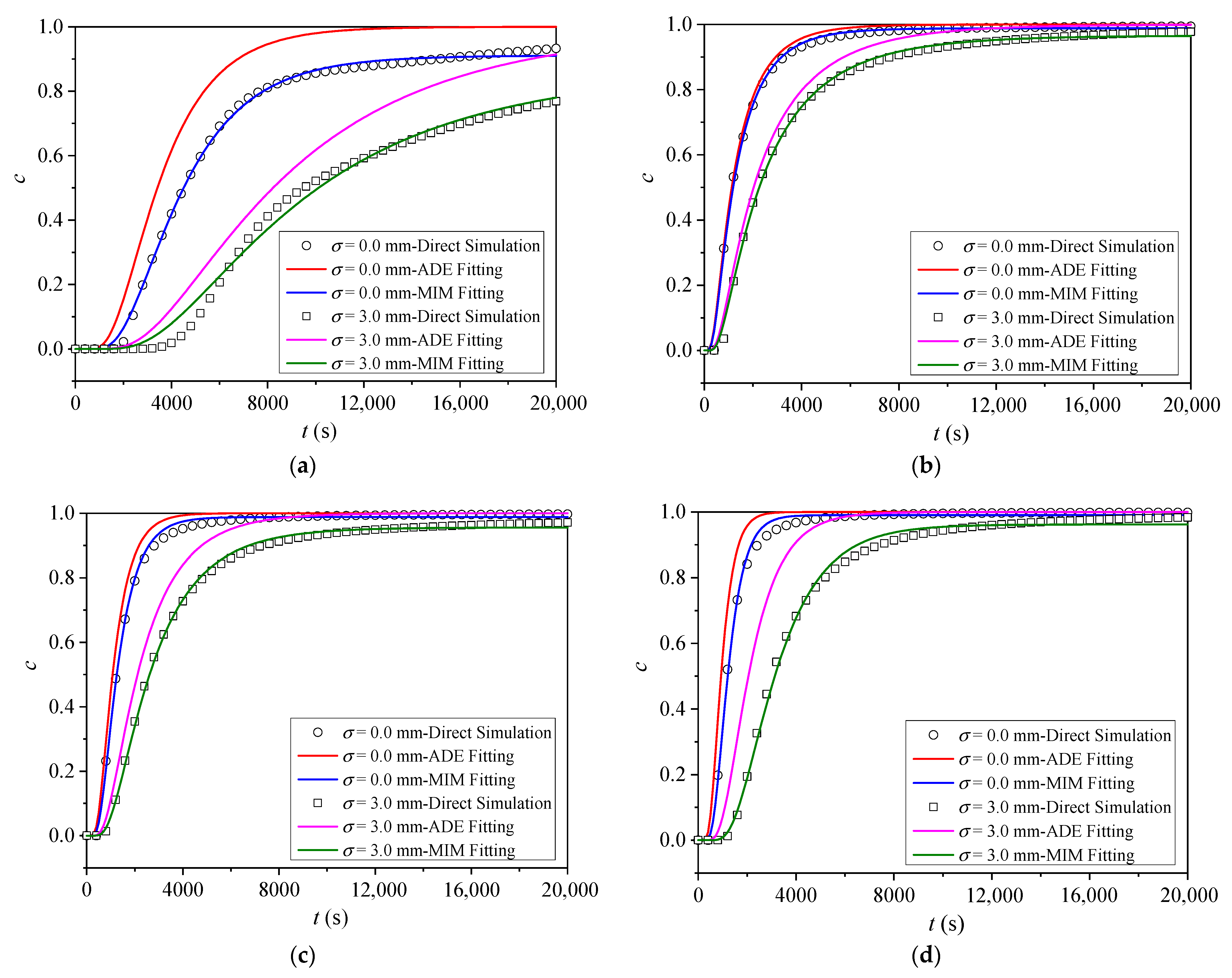
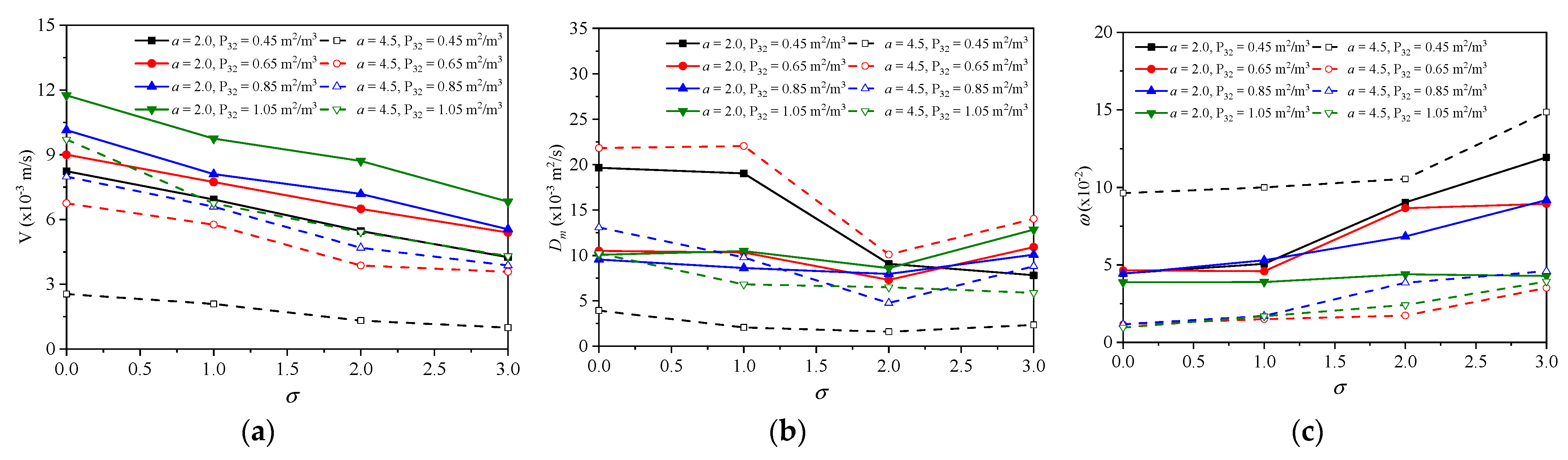
3.3. Inverse Model for BTCs

To further analyze the combined influences of network topology and aperture heterogeneity on the solute transport, the ADE model and MIM model were utilized to fit the BTCs for DFNs possessing different P₃₂ and a, as shown in Figure 10 and Figure 11. The global errors of fitting results using the ADE and MIM models are tabulated in

Table 1. The global error of fitting results using ADE and MIM models.

P32 (m2/m3)	σ	a = 2.0		a = 4.5
		EADE	EMIM	EADE	EMIM
0.45	0	0.0529	0.0323	0.0478	0.0345
0.45	1	0.0345	0.0188	0.0292	0.0108
0.45	2	0.0779	0.0268	0.0277	0.0145
0.45	3	0.0342	0.0191	0.0524	0.0345
0.65	0	0.0517	0.0403	0.0213	0.015
0.65	1	0.0324	0.0249	0.0251	0.0174
0.65	2	0.0512	0.0382	0.0266	0.0186
0.65	3	0.0309	0.0236	0.028	0.0136
0.85	0	0.043	0.0323	0.0226	0.0142
0.85	1	0.0394	0.0304	0.0268	0.0166
0.85	2	0.0446	0.0346	0.0133	0.0085
0.85	3	0.0311	0.0234	0.0290	0.0196
1.05	0	0.0497	0.0360	0.0441	0.0256
1.05	1	0.0321	0.0218	0.0358	0.0269
1.05	2	0.0434	0.0337	0.0436	0.0298
1.05	3	0.0318	0.0233	0.0426	0.0328

. The deviation between the calculated curve and the predicted results based on ADE model is more obvious with a larger E_ADE compared to the MIM model. The ADE model cannot properly characterize the evolution of BTCs. In addition, the deviation between the fitting data and simulation results increases as σ increases, since the phenomenon of preferential transport paths becomes more obvious in the more heterogeneous aperture field. In contrast, the MIM model shows better fitting results with a smaller E_MIM for all cases compared to the ADE model, especially when capturing the long tails of BTCs. This can also be reflected by comparing the global error shown in Table 1. Overall, by separating the liquid phase into flowing and stagnate regions, the MIM model is proven to better fit the BTCs of 3D DFNs with heterogeneous aperture.

The best-fitted parameters of V and D_m and ω for the MIM models are summarized in Figure 12. Figure 12a indicates that with increasing σ, V consistently decreases approximately following a linear relationship. For DFNs possessing the same P₃₂, a larger a would result in a smaller V, and this reduction effect is weakened as P₃₂ increases. As shown in Figure 12b, D_L gradually decreases as σ increases from 0 to 2.0, and then slightly increases as σ continuously increases to 3.0. As P₃₂ increases or a decreases, the discrepancy of D_L induced by different σ decreases. This is because the increases in fracture density and fracture length would enhance the network connectivity, which would weaken the unfavorable influence induced by aperture heterogeneity on the solute migration. Combined with Figure 12a,b, it can be seen that the decrease in flow velocity tends to weaken the dispersion effect, while the increase in σ enhancing the channeling flow would promote the dispersion. The final result of D_L depends on the combination of those two effects. Figure 12c indicates that ω generally increases as σ increases, which also indicates that the more obvious flow channeling induced by a larger σ enhances the dispersion inside the fractures. This enhancement is commonly more obvious for DFNs with a larger fracture length.

4. Conclusions

A series of 3D DFN models that have different fracture density, length, and aperture distribution were constructed in this study to investigate the effects of topological properties with local variable apertures on solute transport through fractured rock masses. Fluid flow and solute transport through 3D DFNs were numerically simulated based on MATLAB code and COMSOL Multiphysics. Evolutions of flow rate and concentration field in 3D DFNs with heterogeneous apertures were simulated. The reliability of the ADE and MIM models in describing the BTCs of 3D DFNs were compared.

The results indicate that there exists obvious preferential flow within the 3D DFNs, and this phenomenon is more pronounced in fracture networks with heterogeneous aperture than those with identical aperture. The spatial evolutions of concentration fields are found to be sensitive to those flow channels. The solute moves faster in the high-flow channels than in the low-flow regions, showing that the concentration field forms advection channels along the preferential flow paths. For the DFN with a relatively small fracture density, the available flow and transport paths decrease with increasing the fracture length exponent, whereas for dense the DFNs, increasing the fracture length exponent does not cause drastic change in the network connectivity, but rather adds smaller fractures to the existing connected pathways, which would not alter the flow and transport channels significantly. As fracture density increases, the BTCs shift towards the left, which indicates that the arrival time of the DFNs with denser fractures is earlier than that of those with sparse fractures due to more available flow paths. As the aperture heterogeneity increases, the BTCs slightly lag behind because the low velocity in the small-aperture regions hinder the flow and solute migration. The ADE model cannot properly capture the evolution of the BTCs for the 3D DFNs, especially its long tails. Compared with the ADE model, the MIM model, separating the liquid phase into flowing and stagnate regions, is proven to better fit the BTCs of the 3D DFNs with heterogeneous aperture. The best-fitted flow velocity for the ADE and MIM models consistently decreases as aperture heterogeneity increases, approximately following a linear relationship. The best-fitted dispersion coefficient decreases first and then slightly increases as aperture heterogeneity increases. Increasing the aperture heterogeneity tends to decrease the flow velocity and thus the dispersion effect, while it can also enhance the channeling flow thereby promoting the dispersion. As a result, the final magnitude of the dispersion coefficient depends on the combination of those two competing effects. These results may provide a basis for more precise modeling to the improve the simulation accuracy of solute transport in fractured media. The topological properties of the DFNs generated in this study are assumed to follow some statistical distributions with different characteristic exponents which are not compared to the field observation. In the future, when more field data become available, realistic models with geometries similar to natural fractured rock masses will be established to quantify the effect of fracture properties on solute transport from a general perspective.

References

1. Blum, P.; Mackay, R.; Riley, M.S.; Knight, J.L. Performance assessment of a nuclear waste repository: Upscaling coupled hydro-mechanical properties for far-field transport analysis. Int. J. Rock Mech. Min. Sci. 2005, 42, 781–792. [Google Scholar] [CrossRef]
2. Hadgu, T.; Karra, S.; Kalinina, E.; Makedonska, N.; Hyman, J.D.; Klise, K.; Wang, Y. A comparative study of discrete fracture network and equivalent continuum models for simulating flow and transport in the far field of a hypothetical nuclear waste repository in crystalline host rock. J. Hydrol. 2017, 553, 59–70. [Google Scholar] [CrossRef]
3. Lee, I.H.; Ni, C.F. Fracture-based modeling of complex flow and CO2 migration in three-dimensional fractured rocks. Comput. Geosci. 2015, 81, 64–77. [Google Scholar] [CrossRef]
4. Carroll, S.; Carey, J.W.; Dzombak, D.; Huerta, N.J.; Li, L.; Richard, T.; Um, W.; Walsh, S.D.C.; Zhang, L. Role of chemistry, mechanics, and transport on well integrity in CO2 storage environments. Int. J. Greenh. Gas Control 2016, 49, 149–160. [Google Scholar] [CrossRef]
5. Gao, Q.; Ghassemi, A. Three-dimensional thermo-poroelastic modeling and analysis of flow, heat transport and deformation in fractured rock with applications to a lab-scale geothermal system. Rock Mech. Rock Eng. 2020, 53, 1565–1586. [Google Scholar] [CrossRef]
6. Huang, Y.; Pang, Z.; Kong, Y.; Watanabe, N. Assessment of the high-temperature aquifer thermal energy storage (HT-ATES) potential in naturally fractured geothermal reservoirs with a stochastic discrete fracture network model. J. Hydrol. 2021, 603, 127188. [Google Scholar] [CrossRef]
7. Nemoto, K.; Watanabe, N.; Hirano, N.; Tsuchiya, N. Direct measurement of contact area and stress dependence of anisotropic flow through rock fracture with heterogeneous aperture distribution. Earth Planet. Sci. Lett. 2009, 281, 81–87. [Google Scholar] [CrossRef]
8. Liu, R.; Li, B.; Jiang, Y. Critical hydraulic gradient for nonlinear flow through rock fracture networks: The roles of aperture, surface roughness, and number of intersections. Adv. Water Resour. 2016, 88, 53–65. [Google Scholar] [CrossRef]
9. Huang, N.; Zhang, Y.; Yin, Q.; Jiang, Y.; Liu, R. Combined Effect of Contact Area, Aperture Variation, and Fracture Connectivity on Fluid Flow through Three-Dimensional Rock Fracture Networks. Lithosphere 2022, 2022, 2097990. [Google Scholar] [CrossRef]
10. Kobayashi, A.; Chijimatsu, M. Continuous modeling of transport phenomena through fractured rocks. Soils Found. 1998, 38, 41–53. [Google Scholar] [CrossRef] [PubMed]
11. Svensson, U. A continuum representation of fracture networks. Part I: Method and basic test cases. J. Hydrol. 2001, 250, 170–186. [Google Scholar]
12. Marina, S.; Derek, I.; Mohamed, P.; Yong, S.; Imo-Imo, E.K. Simulation of the hydraulic fracturing process of fractured rocks by the discrete element method. Environ. Earth Sci. 2015, 73, 8451–8469. [Google Scholar] [CrossRef]
13. Xia, L.; Zheng, Y.; Yu, Q. Estimation of the REV size for blockiness of fractured rock masses. Comput. Geotech. 2016, 76, 83–92. [Google Scholar] [CrossRef]
14. Rutqvist, J.; Figueiredo, B.; Hu, M.; Tsang, C.F. Continuum modeling of hydraulic fracturing in complex fractured rock masses. In Hydraulic Fracture Modeling; Gulf Professional Publishing: Houston, TX, USA, 2018; pp. 195–217. [Google Scholar]
15. Berkowitz, B.; Scher, H. Theory of anomalous chemical transport in random fracture networks. Phys. Rev. E 1998, 57, 5858. [Google Scholar] [CrossRef]
16. Jing, L. Block system construction for three-dimensional discrete element models of fractured rocks. Int. J. Rock Mech. Min. Sci. 2000, 37, 645–659. [Google Scholar] [CrossRef]
17. Lei, Q.; Latham, J.P.; Xiang, J.; Tsang, C.F.; Lang, P.; Guo, L. Effects of geomechanical changes on the validity of a discrete fracture network representation of a realistic two-dimensional fractured rock. Int. J. Rock Mech. Min. Sci. 2014, 70, 507–523. [Google Scholar] [CrossRef]
18. Lang, P.S.; Paluszny, A.; Zimmerman, R.W. Permeability tensor of three-dimensional fractured porous rock and a comparison to trace map predictions. J. Geophys. Res. Solid Earth 2014, 119, 6288–6307. [Google Scholar] [CrossRef]
19. Ren, F.; Ma, G.; Fan, L.; Wang, Y.; Zhu, H. Equivalent discrete fracture networks for modelling fluid flow in highly fractured rock mass. Eng. Geol. 2017, 229, 21–30. [Google Scholar] [CrossRef]
20. Lee, I.H.; Ni, C.F.; Lin, F.P.; Lin, C.P.; Ke, C.C. Stochastic modeling of flow and conservative transport in three-dimensional discrete fracture networks. Hydrol. Earth Syst. Sci. 2019, 23, 19–34. [Google Scholar] [CrossRef]
21. Huang, N.; Jiang, Y.; Liu, R.; Li, B.; Sugimoto, S. A novel three-dimensional discrete fracture network model for investigating the role of aperture heterogeneity on fluid flow through fractured rock masses. Int. J. Rock Mech. Min. Sci. 2019, 116, 25–37. [Google Scholar] [CrossRef]
22. Akara, M.E.M.; Reeves, D.M.; Parashar, R. Impact of horizontal spatial clustering in two-dimensional fracture networks on solute transport. J. Hydrol. 2021, 603, 127055. [Google Scholar] [CrossRef]
23. Khafagy, M.; El-Dakhakhni, W.; Dickson-Anderson, S. Analytical model for solute transport in discrete fracture networks: 2D spatiotemporal solution with matrix diffusion. Comput. Geosci. 2022, 159, 104983. [Google Scholar] [CrossRef]
24. Maillot, J.; Davy, P.; Le Goc, R.; Darcel, C.; De Dreuzy, J.R. Connectivity, permeability, and channeling in randomly distributed and kinematically defined discrete fracture network models. Water Resour. Res. 2016, 52, 8526–8545. [Google Scholar] [CrossRef]
25. Frampton, A.; Hyman, J.D.; Zou, L. Advective transport in discrete fracture networks with connected and disconnected textures representing internal aperture variability. Water Resour. Res. 2019, 55, 5487–5501. [Google Scholar] [CrossRef]
26. Kang, P.K.; Hyman, J.D.; Han, W.S.; Dentz, M. Anomalous transport in three-dimensional discrete fracture networks: Interplay between aperture heterogeneity and injection modes. Water Resour. Res. 2020, 56, e2020WR027378. [Google Scholar] [CrossRef]
27. Makedonska, N.; Painter, S.L.; Bui, Q.M.; Gable, C.W.; Karra, S. Particle tracking approach for transport in three-dimensional discrete fracture networks: Particle tracking in 3-D DFNs. Comput. Geosci. 2015, 19, 1123–1137. [Google Scholar] [CrossRef]
28. Ngo, T.D.; Fourno, A.; Noetinger, B. Modeling of transport processes through large-scale discrete fracture networks using conforming meshes and open-source software. J. Hydrol. 2017, 554, 66–79. [Google Scholar] [CrossRef]
29. Zhao, Z.; Li, B.; Jiang, Y. Effects of fracture surface roughness on macroscopic fluid flow and solute transport in fracture networks. Rock Mech. Rock Eng. 2014, 47, 2279–2286. [Google Scholar] [CrossRef]
30. Dronfield, D.G.; Silliman, S.E. Velocity dependence of dispersion for transport through a single fracture of variable roughness. Water Resour. Res. 1993, 29, 3477–3483. [Google Scholar] [CrossRef]
31. Johnson, J.; Brown, S. Experimental mixing variability in intersecting natural fractures. Geophys. Res. Lett. 2001, 28, 4303–4306. [Google Scholar] [CrossRef]
32. Roux, S.; Plouraboué, F.; Hulin, J.P. Tracer dispersion in rough open cracks. Transp. Porous Media 1998, 32, 97–116. [Google Scholar] [CrossRef]
33. Larsson, M.; Odén, M.; Niemi, A.; Neretnieks, I.; Tsang, C.F. A new approach to account for fracture aperture variability when modeling solute transport in fracture networks. Water Resour. Res. 2013, 49, 2241–2252. [Google Scholar] [CrossRef]
34. Zou, L.; Cvetkovic, V. Impact of normal stress-induced closure on laboratory-scale solute transport in a natural rock fracture. J. Rock Mech. Geotech. Eng. 2020, 12, 732–741. [Google Scholar] [CrossRef]
35. Zhou, J.Q.; Li, C.; Wang, L.; Tang, H.; Zhang, M. Effect of slippery boundary on solute transport in rough-walled rock fractures under different flow regimes. J. Hydrol. 2021, 598, 126456. [Google Scholar] [CrossRef]
36. Qian, J.Z.; Chen, Z.; Zhan, H.B.; Luo, S.H. Solute transport in a filled single fracture under non-Darcian flow. Int. J. Rock Mech. Min. Sci. 2011, 48, 132–140. [Google Scholar] [CrossRef]
37. Geiger, S.; Cortis, A.; Birkholzer, J.T. Upscaling solute transport in naturally fractured porous media with the continuous time random walk method. Water Resour. Res. 2010, 46, W12530. [Google Scholar] [CrossRef]
38. Nowamooz, A.; Radilla, G.; Fourar, M.; Berkowitz, B. Non-Fickian transport in transparent replicas of rough-walled rock fractures. Transp. Porous Media 2013, 98, 651–682. [Google Scholar] [CrossRef]
39. Bauget, F.; Fourar, M. Non-Fickian dispersion in a single fracture. J. Contam. Hydrol. 2008, 100, 137–148. [Google Scholar] [CrossRef] [PubMed]
40. Dou, Z.; Sleep, B.; Zhan, H.; Zhou, Z.; Wang, J. Multiscale roughness influence on conservative solute transport in self-affine fractures. Int. J. Heat Mass Transf. 2019, 133, 606–618. [Google Scholar] [CrossRef]
41. Hu, Y.; Xu, W.; Zhan, L.; Zou, L.; Chen, Y. Modeling of solute transport in a fracture-matrix system with a three-dimensional discrete fracture network. J. Hydrol. 2022, 605, 127333. [Google Scholar] [CrossRef]
42. Cherubini, C.; Giasi, C.I.; Pastore, N. On the reliability of analytical models to predict solute transport in a fracture network. Hydrol. Earth Syst. Sci. 2014, 18, 2359–2374. [Google Scholar] [CrossRef]
43. Lei, Q.; Latham, J.P.; Tsang, C.F.; Xiang, J.; Lang, P. A new approach to upscaling fracture network models while preserving geostatistical and geomechanical characteristics. J. Geophys. Res. Solid Earth 2015, 120, 4784–4807. [Google Scholar] [CrossRef]
44. Darcel, C.; Bour, O.; Davy, P. Stereological analysis of fractal fracture networks. J. Geophys. Res. Solid Earth 2003, 108, 2451. [Google Scholar] [CrossRef]
45. De Dreuzy, J.R.; Méheust, Y.; Pichot, G. Influence of fracture scale heterogeneity on the flow properties of three-dimensional discrete fracture networks (DFN). J. Geophys. Res. Solid Earth 2012, 117, B11207. [Google Scholar] [CrossRef]
46. Detwiler, R.L.; Pringle, S.E.; Glass, R.J. Measurement of fracture aperture fields using transmitted light: An evaluation of measurement errors and their influence on simulations of flow and transport through a single fracture. Water Resour. Res. 1999, 35, 2605–2617. [Google Scholar] [CrossRef]
47. Isakov, E.; Ogilvie, S.R.; Taylor, C.W.; Glover, P.W. Fluid flow through rough fractures in rocks I: High resolution aperture determinations. Earth Planet. Sci. Lett. 2001, 191, 267–282. [Google Scholar] [CrossRef]
48. Lapcevic, P.A.; Novakowski, K.S.; Sudicky, E.A. The interpretation of a tracer experiment conducted in a single fracture under conditions of natural groundwater flow. Water Resour. Res. 1999, 35, 2301–2312. [Google Scholar] [CrossRef]
49. Brown, S.R.; Kranz, R.L.; Bonner, B.P. Correlation between the surfaces of natural rock joints. Geophys. Res. Lett. 1986, 13(13), 1430–1433. [Google Scholar] [CrossRef]
50. Masciopinto, C. Pumping-well data for conditioning the realization of the fracture aperture field in groundwater flow models. J. Hydrol. 2005, 309, 210–228. [Google Scholar] [CrossRef]
51. Bonnet, E.; Bour, O.; Odling, N.E.; Davy, P.; Main, I.; Cowie, P.; Berkowitz, B. Scaling of fracture systems in geological media. Rev. Geophys. 2001, 39, 347–383. [Google Scholar] [CrossRef]
52. Li, B.; Wang, J.; Liu, R.; Jiang, Y. Nonlinear fluid flow through three-dimensional rough fracture networks: Insights from 3D-printing, CT-scanning, and high-resolution numerical simulations. J. Rock Mech. Geotech. Eng. 2021, 13, 1020–1032. [Google Scholar] [CrossRef]
53. Foias, C.; Manley, O.; Rosa, R.; Temam, R. Navier-Stokes Equations and Turbulence; Cambridge University Press: Cambridge, UK, 2001; Volume 83. [Google Scholar]
54. Witherspoon, P.A.; Wang, J.S.; Iwai, K.; Gale, J.E. Validity of cubic law for fluid flow in a deformable rock fracture. Water Resour. Res. 1980, 16, 1016–1024. [Google Scholar] [CrossRef]
55. Bear, J. Dynamics of Fluids in Porous Media; Courier Corporation: Chelmsford, MA, USA, 2013. [Google Scholar]
56. De Marsily, G. Quantitative Hydrogeology; Paris School of Mines: Fontainebleau, France, 1986. [Google Scholar]
57. Cherubini, C.; Giasi, C.I.; Pastore, N. Evidence of non-Darcy flow and non-Fickian transport in fractured media at laboratory scale. Hydrol. Earth Syst. Sci. 2013, 17, 2599–2611. [Google Scholar] [CrossRef]
58. Parker, J.C.; Van Genuchten, M.T. Flux-averaged and volume-averaged concentrations in continuum approaches to solute transport. Water Resour. Res. 1984, 20, 866–872. [Google Scholar] [CrossRef]
59. Thompson, M.E. Numerical simulation of solute transport in rough fractures. J. Geophys. Res. Solid Earth 1991, 96, 4157–4166. [Google Scholar] [CrossRef]
60. Dou, Z.; Chen, Z.; Zhou, Z.; Wang, J.; Huang, Y. Influence of eddies on conservative solute transport through a 2D single self-affine fracture. Int. J. Heat Mass Transf. 2018, 121, 597–606. [Google Scholar] [CrossRef]
61. Tang, G.; Mayes, M.A.; Parker, J.C.; Jardine, P.M. CXTFIT/Excel–A modular adaptable code for parameter estimation, sensitivity analysis and uncertainty analysis for laboratory or field tracer experiments. Comput. Geosci. 2010, 36, 1200–1209. [Google Scholar] [CrossRef]
Figure 1. Generated 3D DFN models with different fracture density P32 and fracture length exponent a.
Processes 11 03157 g001
Figure 2. Frequency of aperture distributions with different deviation: (a) bm = 1.72 mm, σ = 1.0 mm, (b) bm = 1.72 mm, σ = 2.0 mm, and (c) bm = 1.72 mm, σ = 3.0 mm.
Processes 11 03157 g002
Figure 3. (a) Triangular mesh of the 3D DFNs with conforming constraint at fracture intersections, and (b) boundary conditions for the simulation of flow and transport.
Processes 11 03157 g003
Figure 4. Flow rate (ad) and concentration field (el) at t = 1000 s and t = 3000 s in the 3D DFNs with different fracture densities when a = 2.0 and σ = 0 mm.
Processes 11 03157 g004
Figure 5. Evolutions of BTCs with fracture densities for 3D DFNs having different aperture distributions: (a) a = 2.0, σ = 0.0 mm, (b) a = 2.0, σ = 1.0 mm, (c) a = 2.0, σ = 2.0 mm, and (d) a = 2.0, σ = 3.0 mm.
Processes 11 03157 g005
Figure 6. Flow rate (ad) and concentration field (el) at t = 1000 s and t = 3000 s in the 3D DFNs with different fracture densities when a = 4.5 and σ = 0 mm.
Processes 11 03157 g006
Figure 7. Evolutions of BTCs with fracture length exponent for 3D DFNs having different fracture densities: (a) P32 = 0.45 m2/m3, σ = 0 mm, (b) P32 = 0.65 m2/m3, σ = 0 mm, (c) P32 = 0.85 m2/m3, σ = 0 mm, (d) P32 = 1.05 m2/m3, σ = 0 mm.
Processes 11 03157 g007
Figure 8. Aperture (ad), flow rate (eh), and concentration field (ip) at t = 1000 s and t = 3000 s in the 3D DFNs with different aperture distribution when a = 2.0 and P32 = 0.65 m2/m3.
Processes 11 03157 g008
Figure 9. Evolutions of BTCs with fracture aperture distribution for 3D DFNs having different fracture densities: (a) a = 2.0, P32 = 0.45 m2/m3, (b) a = 2.0, P32 = 0.65 m2/m3, (c) a = 2.0, P32 = 0.85 m2/m3, (d) a = 2.0, P32 = 1.05 m2/m3.
Processes 11 03157 g009
Figure 10. Best fitted results of BTCs for 3D DFNs with a = 2.0 using ADE and MIM models: (a) P32 = 0.45 m2/m3, (b) P32 = 0.65 m2/m3, (c) P32 = 0.85 m2/m3, and (d) P32 = 1.05 m2/m3.
Processes 11 03157 g010
Figure 11. Best fitted results of BTCs for 3D DFNs with a = 4.5 using ADE and MIM models: (a) P32 = 0.45 m2/m3, (b) P32 = 0.65 m2/m3, (c) P32 = 0.85 m2/m3, and (d) P32 = 1.05 m2/m3.
Processes 11 03157 g011
Figure 12. Best-fitted results of MIM model for 3D DFNs with different length exponent: (a) V, (b) Dm, and (c) ω.
Processes 11 03157 g012