Article

Energy Valley Optimizer (EVO) for Tracking the Global Maximum Power Point in a Solar PV System under Shading

1
Department of Electrical Engineering, Zakir Husain College of Engineering and Technology (ZHCET), Aligarh Muslim University, Aligarh 202002, India
2
Department of Electrical Engineering, National Chin-Yi University of Technology, Taichung 411, Taiwan
3
Department of Electrical and Computer Engineering, Florida International University, Miami, FL 33174, USA
4
Industrial Engineering Department, College of Engineering, King Saud University, Riyadh 11421, Saudi Arabia
5
Undergraduate Program of Vehicle and Energy Engineering, National Taiwan Normal University, Taipei 106, Taiwan
6
Department of Electrical Engineering, National Taiwan University of Science and Technology, Taipei 106, Taiwan
*
Authors to whom correspondence should be addressed.
Processes 2023, 11(10), 2986; https://doi.org/10.3390/pr11102986
Submission received: 4 September 2023 / Revised: 4 October 2023 / Accepted: 9 October 2023 / Published: 16 October 2023

Abstract

:
Incorporating bypass diodes within photovoltaic arrays serves to mitigate the negative effects of partial shading scenarios. These situations can lead to the appearance of multiple peaks in the performance of solar panels. Nevertheless, there are cases where conventional maximum power point tracking (MPPT) techniques could encounter inaccuracies, causing them to identify the highest power point within a specific area (the local maximum power point; LMPP) instead of the overall highest power point across the entire array (the global maximum power point; GMPP). Numerous methods based on artificial intelligence (AI) were proposed to address this issue; however, they frequently used cumbersome and unreliable methodologies. This research presents the energy-valley-optimizer-based optimization (EVO) technique, which is designed to efficiently and dependably tackle the issue of partial shading (PS) in detecting the maximum power point (MPP) for photovoltaic (PV) systems. The EVO algorithm enhances the speed of tracking and minimizes power output fluctuations during the tracking phase. Through the utilization of the Typhoon hardware-in-the-loop (HIL) 402 emulator, extensive validation of the proposed technique is conducted. The effectiveness of the suggested method is compared with the established cuckoo search algorithm for achieving maximum power point tracking (MPPT) within a photovoltaic (PV) system. This comparison takes place under equivalent conditions to ensure a fair performance evaluation.

1. Introduction

As the global population continues to expand, and the use of electrical technologies becomes more prevalent, the power sector is experiencing mounting challenges to satisfy the rising global energy demands. Yet depending solely on conventional energy sources exacerbates harm to the environment and jeopardizes human welfare. As a result, scholars are shifting their attention toward renewable energy sources like geothermal, solar, biomass, tidal, and wind energy extraction. This shift aims to address the urgent requirement for sustainable energy options. This shift in focus aims to explore and harness the potential of these renewable resources as alternatives to mitigate environmental harm and promote long-term sustainability [1,2,3].
Solar energy has become widely popular because of its numerous advantages, which encompass its eco-friendly nature, minimal need for maintenance, quiet operation, simple execution, and plentiful availability in the natural environment [3]. Due to the benefits of renewable energy, the Indian government announced plans to increase its renewable energy capacity by 50 GW yearly over the next five years to reach the goal of 500 GW by 2030. India presently has 168.96 GW of total renewable energy capacity (as of February 28, 2023), with roughly 82 GW of that capacity being implemented at various phases and over 41 GW being in the bidding stage. As seen in Figure 1, this comprises 64.38 GW of solar power, 51.79 GW of hydropower, 42.02 GW of wind power, and 10.77 GW of biopower [4].
Moreover, the costs associated with establishing photovoltaic (PV) systems are rapidly decreasing because of advancements in PV technologies. The cost of producing one unit of energy has significantly decreased in recent decades due to PV technology advancements. However, there are still several issues with and limits of solar PV technology, including relatively poor power efficiency, non-linearity, a short lifespan, and reliance on environmental variables like insolation and temperature for the best power output [3,5]. Nevertheless, despite these limitations, solar PV technology has a lot of potential as a sustainable energy source.
The power output of a photovoltaic (PV) array can be significantly affected by partial shading (PS) resulting from various factors including shading from buildings, bird droppings, and cloud cover. Moreover, PS has the potential to create hotspots, which can lead to localized damage within the PV module as a result of overheating at specific points. To address the effects of PS, one common approach is to incorporate bypass diodes into the system, although this can sometimes result in multiple peaks on the power and voltage (P-V) curve [6,7]. Numerous optimization techniques, including the use of the maximum power point tracking (MPPT) methodology, were developed to overcome this difficulty. These methods tried to separate the many peaks in the power output that exist from the global maximum power point. The authors of [3] divide MPPT techniques into two main categories: firmware-based methods and hardware-based reconfiguration techniques. Differential power processing (DPP) [8], solar array reconfiguration [9], and DC optimizer techniques [10] are only a few examples of hardware-based reconfiguration systems that have demonstrated excellent performance in tackling this issue. However, these techniques do have some drawbacks. For instance, extra switching mechanisms, skilled staff, and long connections are required to prevent PV module crossover [8]. The usage of numerous DC-to-DC converters is also required by DPP and DC optimizer techniques to regulate power output and handle power level variations across different PV modules [11]. In contrast, firmware-based MPPT methods are gaining notable traction and acceptance. This is primarily due to their capability to identify the GMPP without necessitating extra switching elements or sensors [3]. These methods make use of MPPT controllers that run the PV array at its GMPP by using optimization algorithms. This strategy requires no extra equipment, is simple to apply, and lowers the cost of power generation [12]. Deterministic approaches, intelligent-based techniques, and metaheuristic algorithms are the three primary categories into which MPPT control techniques are divided in the extant literature [12].
Traditional or deterministic MPPT techniques, including Perturb and Observe (P&O) [13], incremental conductance (INC) [14], and Fractional Open Circuit Voltage (FOCV) [15] algorithms, suffer from several limitations. These limitations include inadequate convergence, a tendency to converge to the LMPP under shaded conditions, and fluctuations around the maximum power point. To overcome these challenges, researchers developed artificial intelligence (AI)-based techniques that aim to achieve higher efficiency in dynamic weather conditions. These techniques include artificial neural networks (ANNs) [16], fuzzy logic controllers (FLCs) [17], and evolutionary algorithms (EAs) [18]. Although these techniques have excellent tracking speeds and efficiency, they frequently need intricate control circuits and a lot of data processing for system training. A fuzzy logic controller (FLC) distinguishes itself by enabling MPPT implementation without the need for prior system knowledge. In contrast, artificial neural networks (ANNs) are highly efficient tracking methods that require substantial amounts of training data to enhance accuracy. ANN-based techniques utilize dynamic inputs such as insolation and temperature, which are archived as datasets [19]. The algorithms mentioned above alleviate the storage and computational load on the microprocessor. They also mitigate inaccurate outcomes arising from data gaps or irregularities, which are difficulties associated with vast training data and are relevant to MPPT applications.
Bio-inspired MPPT algorithms like the cuckoo search algorithm (CSA) [20], Flying Squirrel Search Optimization Strategy (FSSO) [21], and owl search algorithm (OSA) [22]. Overall, the recent Bio-Inspired Algorithm for MPPT brings significant advantages in terms of global optimization, adaptability, robustness, and parallel processing. However, it is essential to consider the computational complexity, parameter tuning requirements, and convergence speed when applying these algorithms in practice.
Numerous metaheuristic algorithms were put forward for the optimization of boost converter parameters in the context of MPPT for photovoltaic (PV) systems. These algorithms encompass particle swarm optimization (PSO) [23], the Dandelion Optimizer (DO) [24], driving training-based optimization (DTBO) [25], the emperor penguin optimizer (EPO) [26], Adaptive JAYA (AJAYA) [5], the Giant Trevally Optimizer (GTO) [27], Artificial Rabbits Optimization (ARO) [28], and the Liver Cancer Algorithm (LCA) [29]. These algorithms are designed to increase the likelihood of reaching the GMPP. However, there are certain restrictions on how metaheuristic algorithms may be utilized in MPPT for PV systems. The lack of theoretical guarantees for convergence to the global optimum solution is one of them. Furthermore, there are other factors to consider, such as the gradual rate of convergence, the requirement to adjust multiple parameters for the optimal results, the susceptibility of the initial conditions causing less-than-ideal solutions, the intricacy of implementation demanding substantial computational capacity, and the susceptibility to the initial conditions. Given its quick calculation, straightforward design, parallel processing capabilities, resilience, simplicity, and ease of implementation, the PSO algorithm is one of these metaheuristic algorithms that is frequently used in MPPT applications [30]. It also has a high likelihood of discovering the best overall solution. It is particularly desirable for applications involving multiple-peak functions, making it suitable for MPPT in PV systems [31,32].
Even while PSO increases the likelihood of locating the global peak under shaded circumstances, it does not ensure convergence to the ideal operating zone [33,34]. The PSO-based MPPT algorithm has some limitations. Firstly, it can be time-consuming to track the MPP when dealing with large search spaces [34]. Secondly, it can be challenging to choose the right values for the social and cognitive criteria (c1 and c2), and the inertia factor denoted by w is required to precisely follow the global maxima because the conventional PSO formulation uses random integers, which can reduce search efficiency.
The emperor penguin optimizer (EPO) is used in [26] to assess a novel MPPT control approach under varying irradiance levels and partial shade situations. The movement of penguin agents is principally responsible for EPO. The progress made by this algorithm can be comparatively slower when compared to other optimization methods. The relatively slower convergence speed can negatively affect performance, especially in scenarios where the rapid and accurate identification of the GMPP is critical. This is particularly relevant in situations characterized by rapidly changing irradiance conditions or partial shading, where the need for efficient MPPT is of the utmost importance.
Metaheuristic algorithms, such as PSO, JAYA, and CSA, often face challenges in striking the right balance between exploration and exploitation. These algorithms are intended to find the best answers in challenging search spaces, but they frequently prioritize exploitation, which causes early convergence and traps users in local optima. However, their exploration abilities are frequently poor, which hinders their capacity to find possibly better answers in uncharted portions of the search space [25,35]. The success of an optimization algorithm often depends on its ability to strike the right balance between exploration and exploitation. This balance is crucial because too much exploration can lead to a slow convergence rate, as the algorithm spends too much time searching for new solutions and not enough time exploiting promising ones. Too much exploitation can result in premature convergence to a suboptimal solution, as the algorithm may get stuck in a local optimum without exploring other, potentially better regions of the solution space. Challenges faced by metaheuristic algorithms can arise due to algorithm-specific characteristics, parameter settings, and the nature of the optimization problem being solved. While these algorithms have their strengths, they may not always optimally perform in all scenarios.
Therefore, it becomes essential to achieve a good trade-off between exploration and exploitation when designing and putting these metaheuristic algorithms for MPPT into practice. Their performance and resilience under various environmental situations must be improved. Achieving an optimal balance between exploring new areas of the search space and effectively exploiting the discovered solutions necessitates careful consideration and adjustments.
This paper presents a novel metaheuristic algorithm, named the energy valley optimizer (EVO) algorithm [36], for maximum power point tracking in PV systems. This paper specifically focuses on its application in addressing the partial-shading-conditions problem in solar PV systems, particularly in the context of maximum power point tracking. The development of EVO is inspired by the principles of stability and particle decay found in advanced physics concepts [36]. By utilizing the fundamental principles of particle decay in physics, this study brings a unique perspective to the field. Although this paper presents various examples, it is essential to remember that confirming or denying the superiority of each algorithm requires comprehensive comparisons. In addition, a simulation is conducted to evaluate the effectiveness of the EVO algorithm in various scenarios in the PV system.
Utilizing the EVO algorithm for MPPT in PV systems offers several notable benefits. EVO stands out as a superior choice when compared to other metaheuristic algorithms like PSO, CSA, and the AJAYA algorithm in the following ways:
  • Enhanced Tracking Accuracy: EVO excels at accurately tracking the MPP under varying environmental conditions, including partial shading scenarios. It leverages its unique exploration and exploitation capabilities to swiftly adapt to changing conditions, resulting in a higher tracking accuracy.
  • Improved Convergence Speed: EVO converges to the MPP more quickly than some other algorithms like PSO or CSA. This quicker convergence is crucial for maintaining system efficiency, especially when environmental conditions rapidly change.
  • Robustness in Partial Shading: EVO exhibits robustness when confronted with partial shading conditions. Unlike PSO, which may struggle with premature convergence to local optima in such scenarios, EVO effectively navigates through these challenges, minimizing the impact of shading on energy production.
The arrangement of this research paper is as follows. The formulation and modeling of the photovoltaic (PV) framework are presented in Section 2 of this study. By examining the I-V and P-V curves, Section 3 looks at how changes in solar irradiance affect the output performance of the PV system. Section 4 of this paper outlines the concept of partial shading, while Section 5 offers a description of the framework employed in this study, encompassing maximum power point tracking (MPPT) and a model of the photovoltaic (PV) system. Section 6 provides a detailed explanation of how the proposed EVO-based maximum power point tracking (MPPT) and other metaheuristic algorithms used in this study were implemented. The MATLAB/Simulink results are evaluated and compared in Section 7 and Section 8. In Section 9 and Section 10, the proposed EVO-based MPPT algorithm’s findings are presented together with a comparison with CSA algorithms for the real-time hardware-in-the-loop (HIL) implementation of MPPT. While Section 11 lists potential uses for the recommended method in the future, Section 12 brings this paper to a close.

2. Equivalent Circuit Model of Solar Cell

Solar modules or cells utilize the photoelectric effect to convert energy. A photovoltaic module is comprised of numerous interconnected solar cells arranged in series and/or in parallel configurations to amplify the voltage output and current output. While various solar photovoltaic cell equivalence models exist, this case specifically employs a single-diode model (SDM) for the photovoltaic cell, as shown in Figure 2. PV cells do not act as a current or voltage source themselves but can be likened to a current generator accompanied by a voltage source that relies on it. Within the circuit, there is a parallel connection between a pn junction diode and the current source, along with the presence of a parallel resistance ( R s h ) and a series resistance ( R s ) [37]. Figure 2 illustrates the fundamental representation of the PV cell through the basic single-diode model.
I s     I p h I o   e x p q V o + I s   ·   R s n   ·   K   ·   T 1 V o   + I s   ·   R s R s h
where I s represents the output current; I p h denotes the photoelectric current; the parameter I o corresponds to the diode’s reverse saturation current in the SDM model; the symbol for electric charge is q, whose value is 1.6 × 10 19 Coulomb; V o represents the photovoltaic model’s output voltage; R s denotes the series resistance, while R s h represent the parallel resistance; n signifies the ideality factor; K denotes Boltzmann’s constant; and the temperature of the cell, measured in degrees Celsius, is denoted by the symbol “T”.

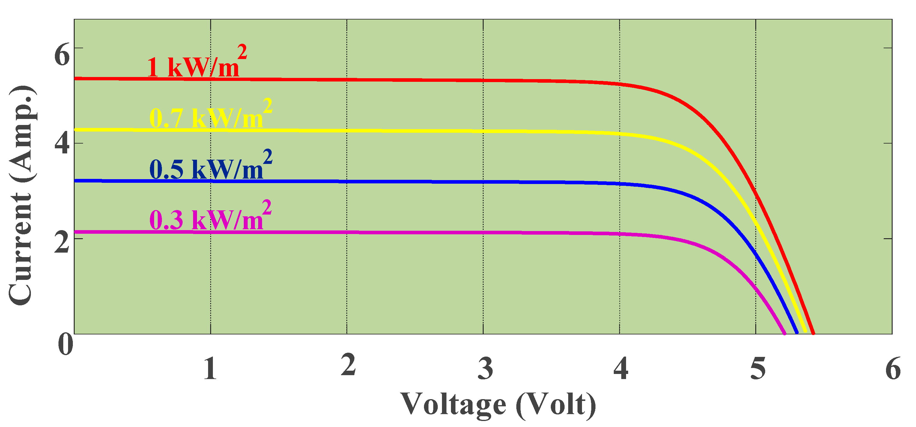
3. Characteristics of Solar Cells

The current that passes through a solar cell when it is connected in a short-circuit arrangement is known as the short-circuit current ( I s c ). In contrast, the open-circuit voltage ( V o c ) is the maximum voltage a solar cell may produce when there is no current flowing through it. The fact that neither the short circuit nor the open circuit states actively contribute to the production of electricity must be understood. However, there is a certain voltage and current combination that optimizes the production of the maximum power ( P m a x ). The behavior of a PV cell at various levels of solar irradiation and constant temperature is shown in Figure 3 and Figure 4. The PV cell’s current–voltage characteristics are shown in Figure 3, and its power–voltage characteristics are shown in Figure 4. According to the conclusions drawn from these graphs, an increase in solar irradiation has little effect on the PV cell’s open-circuit voltage but a considerable influence on its short-circuit current. As a result, at constant temperature, the amount of insolation has a direct impact on the power output of the PV cell.

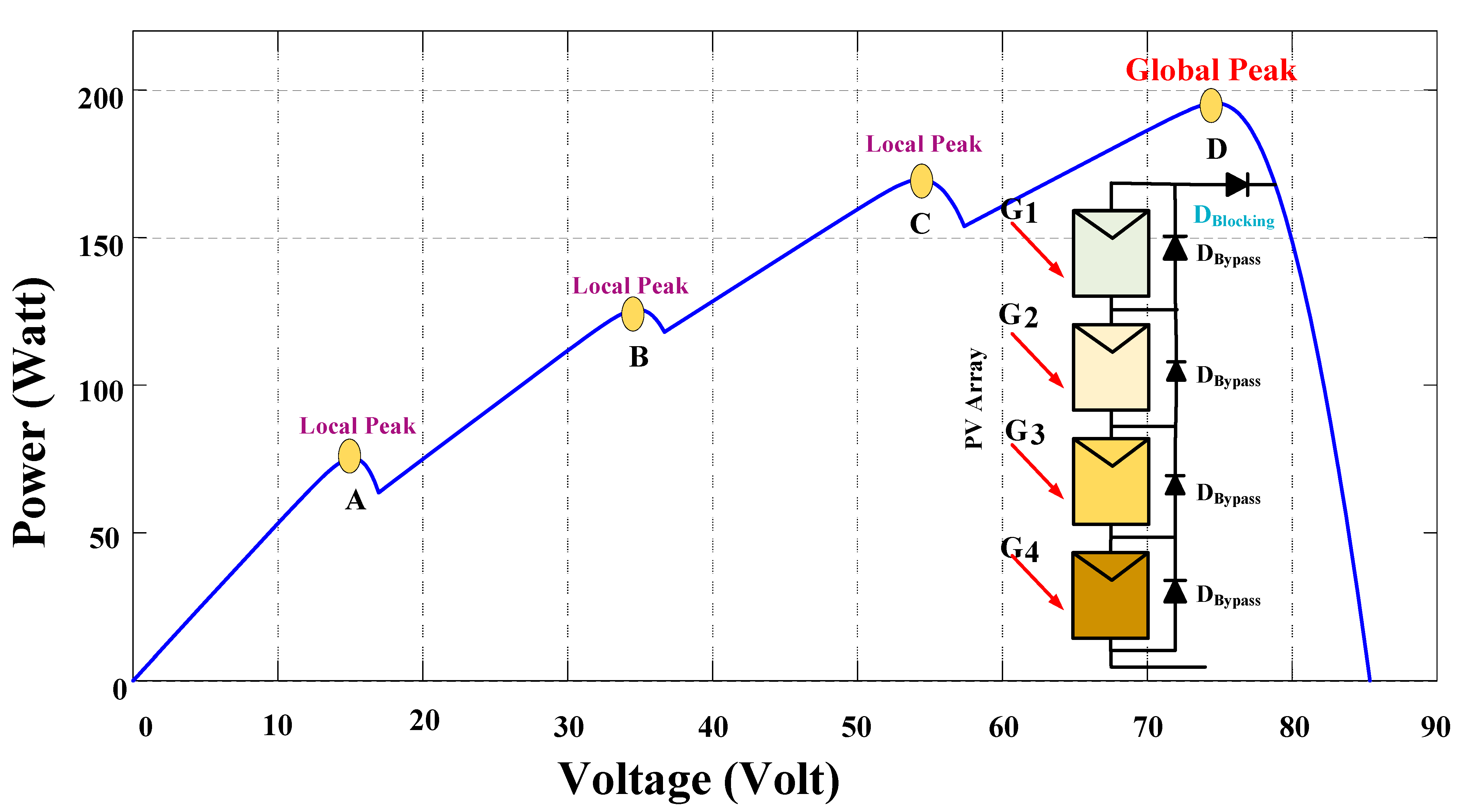
4. PV Array under Partially Shaded Condition

Conventional MPPT methods face a challenge in distinguishing between the local maxima and global maxima, as both points exhibit zero slopes. To address this issue, researchers turned to metaheuristic-based optimization techniques, which are capable of exploring and exploiting the maximum point across the entire search space of the solution vectors. Population-based metaheuristic techniques, such as PSO, emerged as a viable solution to this problem. The following section introduces improved variations of PSO, specifically designed to tackle the power tracking issue in solar PV arrays. Partial shading poses a significant challenge for photovoltaic systems. It occurs when objects obstruct solar rays, casting shadows on surfaces like solar panels and resulting in a partial shading condition (PSC). Consequently, maintaining a consistent and uniform irradiance becomes difficult due to environmental variations such as rain, clouds, storms, and other factors. Additionally, shading from buildings and trees can also contribute to this issue. When solar panels are connected in series, they are susceptible to receiving varying levels of incident irradiance due to the presence of shading [6]. The presence of shading on the PV array causes a reduction in the power generated by the PV module. This decrease in power output is primarily attributed to the non-linear behavior of the module’s output I-V characteristics. The non-linearity leads to the emergence of multiple local maxima on the power–voltage (P-V) curve, further impacting the overall performance and efficiency of the PV system. Understanding these effects is crucial for effectively managing shading issues and optimizing the power-generation capabilities of PV modules. As a result, shading can generate localized areas of excessive heat, known as hot spots, which have the potential to cause significant harm to solar cells. In addition, shading-related problems encompass current mismatches within a PV string and voltage mismatches among parallel modules. The severity of these issues is influenced by several factors, including the configuration of the PV string, the type of modules used, the positioning of bypass diodes, the specific patterns of partial shading, and the intensity of shading. These factors, collectively, determine the extent of the impact caused by shading on the performance of the solar system, as highlighted in [7].
When a PV cell within a string is partially shaded, its current is reduced compared to the unshaded cells. This causes an imbalance in the current distribution, where the unshaded cells start functioning as diodes in the reverse direction. Furthermore, when a cell within a string is shaded, it acts as a hindrance to the overall current flow within the string, leading to a reduction in the output power of the PV string. As more cells within the string are shaded, the reduction in power output becomes more pronounced. The shading effect is addressed by introducing bypass diodes across a specific series of cells within the module. These bypass diodes ensure unidirectional current flow by providing a low-impedance path for power in the designated direction. To effectively mitigate the impact of shading, multiple bypass diodes are connected in an anti-parallel configuration [38].
In this paper, a PV system with four series-connected modules is examined. When partial shading occurs, the current waveform in the I-V curve displays a distinct staircase pattern. Furthermore, Figure 5 illustrates that the corresponding P-V curve exhibits multiple peaks. The presence of non-uniform insolation leads to the observation of four peaks, with one representing the global maximum and the remaining three representing the local maxima.

5. Maximum Power Point (MPP) Tracker

An MPP tracker system, shown in Figure 6, consists of a closed-loop controller coupled with sensors, a microcontroller, a driving circuit, and a DC-to-DC boost converter. The microcontroller measures the voltage and current of the PV array, determines the value of the duty ratio ( D ) , and sends a tuning signal to the converter via the gate driver circuit. The controller utilizes the MPPT algorithm to determine the optimal duty ratio ( D R v a l u e ) values that maximize power extraction ( P m a x ) from the PV array. Equation (2), which stipulates the objective function (z) for the optimization procedure, is used to formulate the MPPT issue.
f D = P m a x
In this study, the GMPP equates to ( D ) , so the value that results in the greatest power output ( P m a x ) is determined using the EVO method.

6. MPPT Based on Metaheuristic Optimization

Metaheuristic algorithms demonstrated their effectiveness in PV-based power generation systems by accurately identifying and tracking the GMPP during MPPT operations. These algorithms possess the capacity to thoroughly inspect the search space and identify the optimal global solution by leveraging their inherent exploitation capabilities, thus outperforming local optimization approaches. Consequently, the choice of optimization algorithm significantly impacts the effectiveness of the MPPT controller. It is crucial to consider several characteristics while creating an MPPT controller to make it both cost- and power-efficient. These parameters are as follows:
  • Minimal failure rate: There should be little chance of early convergence or failure for the MPPT algorithm. The minimal failure rate is determined by dividing the total number of attempts by the number of efforts that converged to one of the MPPs.
  • Rapid convergence: An economic MPP tracker should use fewer computing rounds since the MPPT method should soon settle at the MPP.
  • Consistent fluctuations: The MPPT algorithm should possess dependable abilities for both exploring and exploiting the search space, avoiding the unnecessary traversal of irrelevant regions. As a result, power fluctuations and related losses are decreased.
  • Resilience: Even in the presence of significant oscillations under PS circumstances and abrupt dynamic changes in PV insolation, the MPPT algorithm should be able to identify the GMPP.
It is crucial to look into and use cutting-edge algorithms that may improve crucial elements like convergence speed, reduced power fluctuations, and increased computational efficiency to guarantee the efficient operation of an MPPT controller. Through the use of metaheuristic algorithms, the MPPT technique may be described. In this method, the MPPT issue may be resolved by adjusting the duty ratio of the DC-to-DC boost converter. Starting the process involves building the metaheuristic algorithm into the microcontroller starting power and duty ratios. The gate driver circuit is used by the MPPT algorithm to activate the boost converter switch after initializing it with the initial duty ratio values. The microcontroller analyzes the voltage ( V p v ) and current ( I p v ) measurements obtained from the sensors. The method records the duty ratio D   corresponding to the maximum power during each iteration by comparing the newly computed power to the prior power. This method determines the ideal duty ratio that maximizes the power extraction for a certain combination of insolation by repeatedly comparing the related powers of various duty ratios.

6.1. Particle Swarm Optimization (PSO)-Based MPPT Technique

Particle swarm optimization is a widely utilized method for exploring random searches and optimizing continuous non-linear functions. Introduced by Eberhart and Kennedy in 1995 [23], the PSO approach draws inspiration from the natural behaviors of fish schooling and flocks assembling [39]. In this algorithm, cooperative birds symbolize particles, each striving to find the optimal (best) solution within the search space. These particles possess a fitness value, represented by both a location vector and a velocity vector. Crucially, the magnitude and direction of a particle’s stride are influenced by its fitness value. By harnessing the collective intelligence of these particles, PSO aims to efficiently navigate the problem landscape and converge toward the most favorable outcomes. The fitness value of each particle not only influences its direction but also determines the magnitude of its stride, guiding its movement within the search space. After that, each particle offers a solution by exchanging the knowledge it learned via its unique search process to select the best one. Figure 7 illustrates the major flowchart of the PSO approach.
When using the PSO technique, the search field is first filled with a collection of random solutions (each particle’s location and velocity). Particles use a social and intellectual trade-off to modify their fitness value after each repetition. In addition to the overall best position, each particle also recalls its own personal best among all the other particles. To discover the optimum option, the swarm periodically updates its position (X) and velocity (V). Following the initialization phase, every particle rapidly moves toward the global maximum, aiming for convergence. Equations (3) and (4) [40] define the update rules for the position (X) and velocity (V) of the nth particle in the kth cycle, determining the conditions for their refreshing, and encapsulate the process through which the particle’s position and velocity are updated to ensure the efficient investigation and use of the search space.
V n ( k + 1 ) = ω V n ( k   ) + S 1 A 1   P p ,   B e s t K X n ( k   ) + S 2 A 2   P g ,   B e s t X n ( k ) ,   n   =   1 ,   2 ,   3 ,   .   .   . ,   N
X n ( k + 1 ) = X n ( k ) + V n ( k + 1 ) ,   n   =   1 ,   2 ,   3 ,   .   .   . ,   N
where K represents the total number of iterations; X n refers to the location of the nth particle (X); the velocity of the nth particle in the (k + 1)th iteration is denoted as V n ( k + 1 ) ; the position of the nth particles at the (k + 1)th iteration is symbolized as X n ( k + 1 ) ; ω stands for the weight of inertia; the acceleration coefficients for social and cognitive aspects are represented by S 1   and S 2 , respectively; arbitrary variables and their evaluations, such as A 1 and A 2 , are uniformly distributed within the range of zero–one, ensuring an even distribution across the PSO algorithm; and the notation P p ,   B e s t i represents the individual best location of the nth particle during the Kth repetition, whereas P g ,   B e s t represents the swarm’s optimum position. If a spontaneous condition, like the one described in Equation (5) during initialization, is met, then the update process follows Equation (6) accordingly.
T f ( X n k   ) > T f   ( P p ,   B e s t K )
P p ,   B e s t K = X n k
where Tf represents the target/objective function that requires maximization.

6.2. Cuckoo Search (CS)-Based MPPT Technique

The cuckoo search (CS) method was first presented by Xin-She Yang and Suash Deb in 2009 and has since become a valuable optimization method [20]. Brood parasitism refers to the behavior exhibited by certain cuckoo birds, such as Tapera, which lay their eggs in the nests of other species of birds. This behavior can be categorized into three types: intra-specific, cooperative, and nest takeover [41]. Tapera, being an intelligent bird, imitates the appearance and behavior of the host birds to ensure the survival of its offspring. Utilizing this concept, the CS technique emerged as a powerful meta-heuristic tool for optimization, offering effective solutions across various domains. The CS strategy, depicted in Figure 8, captures the essence of cuckoo birds’ parasitic behavior, establishing a framework for efficient problem solving. Instead of building their nests, cuckoos lay their eggs inside the nests of other birds. Female cuckoos employ a random search strategy to locate the nests of host species that possess egg characteristics resembling their own. They meticulously select the most suitable nest, maximizing the probability of successful hatching and ensuring the propagation of future generations of cuckoos. To increase the likelihood of successful incubation, cuckoos sometimes make multiple attempts and strategically position their eggs within the nest. Occasionally, cuckoos may remove eggs belonging to the host species from the nest. Host birds are susceptible to being deceived and readily accept unfamiliar eggs into their nests. However, if the host bird detects the presence of foreign eggs, it, undoubtedly, eliminates them from the nest. In the most unfavorable circumstances, the host bird may go so far as to destroy the entire nest, leading to the demise of the alien eggs. To implement the CS scheme, the three idealized criteria listed below are used.
  • Every cuckoo bird deposits a solitary egg into a host nest selected at random.
  • The host nest that possesses the finest, superior eggs (referring to the optimal solutions) is responsible for propagating the upcoming generation of cuckoos.
  • The quantity of host nests in the search space remains consistent throughout the process. P f is the possibility that the host bird discovers the foreign egg, and it ranges from 0 to 1.
In the practical implementation of the CS strategy, the particles in the algorithm are metaphorically represented by cuckoo birds, entrusted with the task of exploring and finding solutions. The eggs laid by these cuckoo birds symbolize the solutions generated at each iteration, contributing to the ongoing optimization process. The quest for the nest in the CS strategy can be likened to the search for food. One popular model for determining the movement and direction is known as a Lévy flight, which is represented by certain mathematical functions. In a Lévy flight, the step lengths follow a probability distribution, similar to chaotic wandering. According to the literature [42], the CS algorithm uses the power-law approach to derive the step length from the Lévy distribution.
L e v y ( λ ) = H λ   ,   ( 1 < λ < 3 )
In this context, H indicates the size or length of the step, while λ refers to the power-law index, which represents the variance. It is important to note that the Levy( λ ) function, exhibits an infinite (unlimited) variance. Utilizing Equation (8) to produce new solutions x t c + 1 for a cuckoo defines the Lévy flight.
x t c + 1 = x t c + α   L e v y ( λ ) ,
where x t c + 1 is the new solution, while x t c   is the current solution, α represents the step size that is greater than zero, and “⨁” represents the entry-wise multiplication.
To generate new voltage samples for MPPT, Equation (9) can be used to modify the Lévy flight:
V t c + 1 = V t ( c ) + α ( L e v y ( λ ) ) V t c + 1 = V t ( c ) + q j k 1 λ V B e s t V t
where V t ( c ) represents the voltage of the t(th) particle at the end of the c(th) iteration; the letter q stands for the Lévy multiplication coefficient; and the values of j and k are determined using the standard distribution curve, as illustrated in Equation (10).
h = N ( 0 ,   σ j 2 ) ,   g = N ( 0 ,   σ k 2 )  
σ j = Γ 1 + λ × s i n π × λ 2 Γ 1 + λ 2 × λ × 2 λ 1 2 1 λ   ,   σ k = 1  
where the integral gamma function is denoted by Γ .
All particles use Levy flights to scan the search space in search of the GMPP throughout each iteration cycle. This iterative process persists until the particles converge toward a particular solution. Once all particles converge, indicating that the best solution is reached, the tracking process ceases.

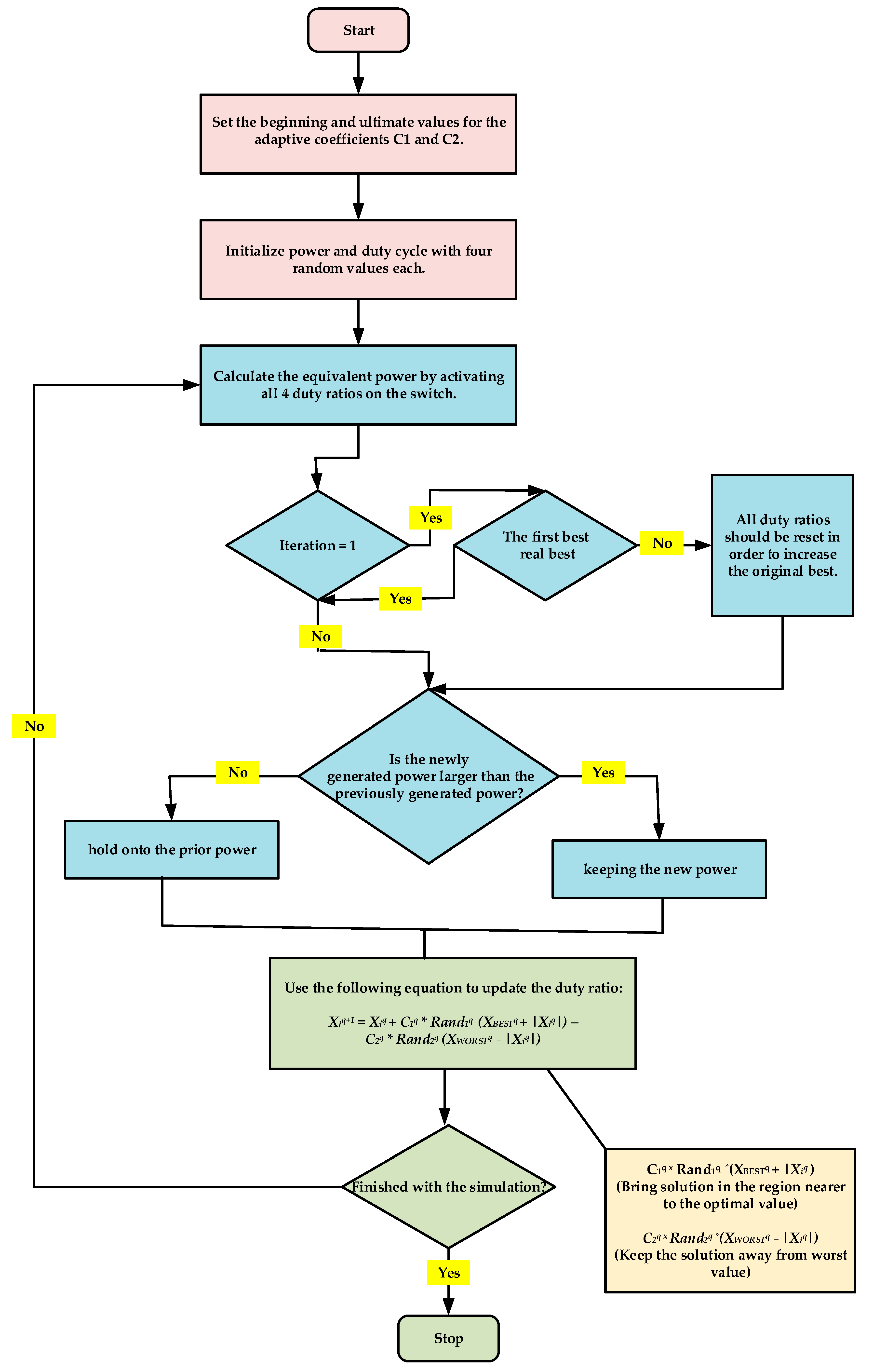
6.3. Adaptive JAYA (AJAYA)-Based MPPT Technique

An enhancement was made to the basic version of the JAYA algorithm by integrating Adaptive Control (AC), as described in [39], into Equation (1). This modification introduces adaptability into the algorithm, allowing it to dynamically adjust the equation during each iteration based on the values of the worst and best components. This adaptive feature aims to expedite convergence by mitigating the issue of extensive diversification observed in the original JAYA algorithm, which often leads to longer convergence times.
Furthermore, it was noted that the AJAYA algorithm exhibits improved performance when the initially identified optimal value is higher than the true optima. To address this, the algorithm was designed to include a reinitialization step for scenarios where the true optima surpass the initially found optima. In such cases, all the duty ratios are reset to elevate the initially found optima above the true optima. Figure 9 shows the flowchart of the Adaptive JAYA algorithm. Equations (12)–(14) are employed in the implementation of the AJAYA algorithm.
X i q + 1   =   X i q + C 1 q × R a n d 1 q X B E S T q X i q C 2 q × R a n d 2 q X W O R S T q X i q  
In every iteration, the AC is modified as follows:
C 1 q = C 1 ( i ) C 1 ( i ) C 1 ( f ) q q m a x
  C 2 q = C 2 ( f ) C 2 ( f ) C 2 ( i ) q m a x q q m a x
where C 1 ( i ) = C 2 ( i ) = 1 , C 1 ( f ) = 0.5 ,   a n d C 2 ( f ) = 0 .
In the AJAYA algorithm, the present iteration value is denoted by q, while q m a x represents the total number of conducted iterations. Initially, the coefficient C 2 q associated with the Weighted Adaptive Control (WAC) is set to a small value, intentionally reducing its impact on the equation. This adjustment helps mitigate the excessive diversification that can occur at the beginning. In contrast, the coefficient C 1 q , which is linked to the Best Exploration Component (BEC), initially remains high, aiming to bring the solution closer to the optimal solution. After the initial simultaneous influence of both coefficients, all solutions in the AJAYA algorithm converge closer to the optimal value, resulting in a reduced gap between the best and worst values. Since the Weighted Adaptive Control (WAC) is no longer causing significant diversification, the coefficient   C 2 q is increased in the subsequent iteration to slightly amplify its impact. Correspondingly, the coefficient C 1 q is decreased, ensuring that the combined effect updates the solution to approach the optimal value while staying away from the worst solution.

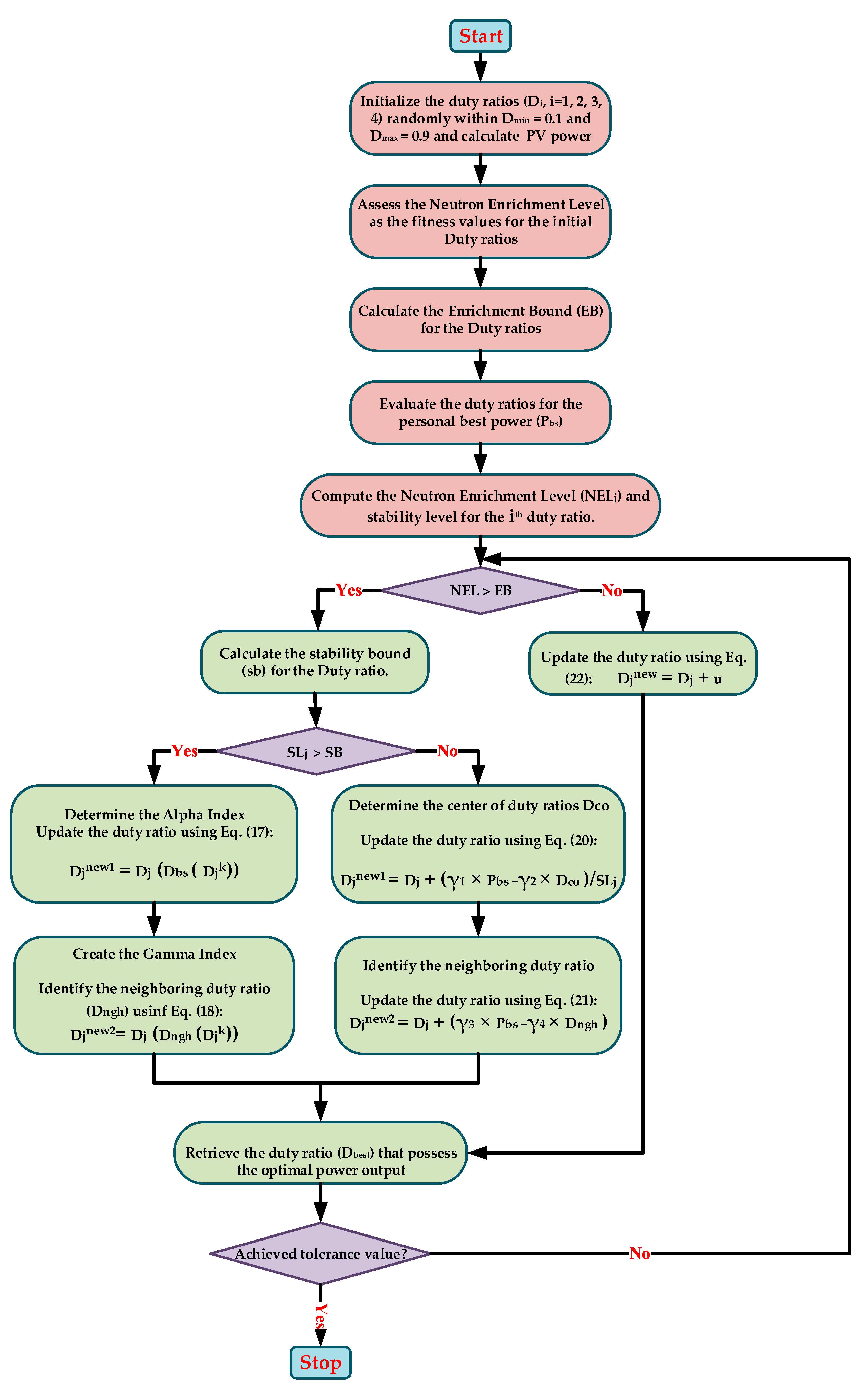
6.4. Energy Valley Optimizer (EVO)-Based MPPT Technique

The existence of multiple metaheuristic algorithms does not diminish the ongoing need for additional ones. These techniques use various methods to search for solutions, particularly when there is not enough information available. The search starts with a small group of randomly chosen candidates, and the metaheuristic techniques incrementally improve their ranking. The principle known as the No Free Lunch (NFL) theory [43] highlights that no single approach can provide a universal solution for all optimization problems. As a result, the continual advancement of new metaheuristic optimization algorithms is imperative to effectively tackle the diverse range of challenges encountered in various problem domains. This pursuit of creating novel metaheuristics offers significant scientific advantages, as they have the potential to enhance the accuracy as well as the efficiency of the optimization process for a diverse set of problems. By introducing innovative metaheuristics, scientists aim to improve the overall efficiency and accuracy of optimization procedures, benefiting various problem domains [36]. Figure 10 depicts the EVO’s flowchart. These techniques use various methods to search for solutions, particularly when there is not enough information available. The search starts with a small group of randomly chosen candidates, and the metaheuristic techniques incrementally improve their ranking.
The proposed EVO algorithm derives its significance from the alignment between the general and advanced principles of physics and its mathematical model, and it draws inspiration from the forefront of physics, specifically concepts related to particle stability and decay [36]. This inspiration catalyzes our innovative approach to addressing optimization challenges. While numerous metaheuristic algorithms exist, the continuous development of new algorithms remains necessary. Introducing novel metaheuristics holds great potential for improving the precision and effectiveness of optimization procedures across various problem domains, especially in maximum power point tracking.

Mathematical Model of Energy Valley Optimizer (EVO)

The previously discussed physics concepts are used to provide a detailed explanation of the EVO as an optimization method in this section. The initialization procedure is carried out in the first phase by randomly assigning values to the duty ratios ( D j k ), where the solution candidates are used to determine the starting position of the jth candidate solution; D j , M i n i m u m k and D j , M a x i m u m k define the lower limit (0.1) and upper limit (0.9) of the kth variable for the jth candidate.
The particles’ enrichment bound (EB) is established in the second phase of the algorithm, and it is used to compare the properties of neutron-rich and neutron-poor particles. The neutron enrichment level (NEL) of particles is calculated for this purpose by completing an objective function assessment of each particle. These aspects are mathematically presented in Equation (15):
Enrichment   Bound = j = 1   g N E L j g ,     j = 1 , 2 , 3 , . . . . g .
where N E L j is the particle’s amount of neutron enrichment, and EB is the universe’s overall enrichment bound.
The third stage establishes the particle stability levels following the assessments of the objective functions, as shown in Equation (16):
S L j = N E L j B S L W S L B S L ,     j = 1 , 2 , 3 , . . . . g .
where the stability status of the jth particle is represented as S L j , while “BSL” and “WSL” pertain to the particles exhibiting the best and lowest stability levels within the entire search space. These correspond to the minimum and maximum values of the objective function identified up to that point.
Within the primary exploration phase of the EVO, the particle’s degree of neutron enrichment is given careful attention. Should this level surpass the established enrichment threshold ( N E L j > EB), it impacts the decay mechanism utilizing alpha, beta, or gamma strategies. Under these circumstances, a random integer within the [0, 1] range is generated to simulate the Stability Bound (SB) of the entire universe. When the stability level of a particle goes beyond the specified stability threshold ( S t a b . L e v e l j > Stability Bound), it is inferred that both alpha and gamma decay processes take place. These decay mechanisms are more probable in the case of larger particles possessing elevated stability levels. Rays are emitted in a manner that enhances the stability of the product throughout the physical progression, following the principles governing alpha decay. This feature may be mathematically expressed as one of the EVO’s position update techniques, where a fresh candidate for a solution is created. Alpha Index I, a random integer within the interval [1, d], denotes the quantity of the rays being released. Similarly, Alpha Index II, chosen randomly from the range [1, Alpha Index I], designates the specific rays to be emitted. These random integers are generated to fulfill this specific objective. The emitted rays within the particle or candidate possessing the best stability level (XBS) are substituted by the rays, which serve as decision variables within the solution candidate. These features are numerically expressed in Equation (17):
D j N e w   1 = D j D B S L . D j k ,                 j = 1 , 2 , 3 , . . . . . . . . g . k = A l p h a   I n d e x   I I .
where D j N e w   1 is the recently generated particle within the universe, D j represents the jth particle’s current location vector in the search space, D j k is denoted by the kth decision variable or emitted ray, and D B S L refers to the positional vector of the particle exhibiting the most optimal stability level. Equation (18) conducts the position update process using these activities to produce the second solution candidate in this phase:
D j N e w   2 = D j D b s   D j k ,                 j = 1 , 2 , 3 , . . . . . . . . . . g . k = G a m m a   I n d e x   I I .
where the variable D j N e w   2 represents the newest particle in the universe; meanwhile, D j represents the present positional vector of the jth particle within the exploration domain. D b s signifies the vector representing the position of the particle’s nearest neighbor, and D j k represents the kth decision variable or emitted photon.
Beta decay is presumed to take place when the stability level of a particle falls below the stability threshold ( S L j > Stability Bound), as this decay type is prevalent among less stable particles characterized by lower stability levels.
In line with the physics principles governing beta decay, particles emit rays to enhance their stability level. Consequently, it is necessary to significantly expand the exploration area, as these particles exhibit heightened levels of instability. In this context, a process of updating positions is executed for the particles. This involves controlled shifts toward both the particle or candidate boasting the highest stability level, represented as D B S L , and the central position of the particle, denoted as D C O P . These aspects of the algorithm replicate the inclination of particles to converge toward the stability region. This area typically houses the bulk of recognized particles, with many displaying elevated levels of stability. These elements are quantitatively expressed in Equations (19) and (20):
D C O P = j = 1   g X j g , j = 1 , 2 , 3 , . . . . g .
D j N e w   1 = P j + u 1 × D B S L u 2 ×   D C O P   S L j
where D j N e w   1 and D j represent the forthcoming and existing positional vectors of the jth particles within the exploration domain. The particle’s positional vector exhibiting the highest stability level is indicated as D B S L , while the position vector for the particle’s center is denoted by D C O P , the stability level of the jth particle is denoted by S t a b . L e v e l j , and u 1 and u 2 are two random numbers in the [0, 1] range that control the amount of particle movement.
Another method of updating positions is carried out for the particles using beta decay to increase the algorithm’s exploitation and exploration levels. In this process, a controlled movement is carried out toward the particle along with the best stability level ( P B S L ) and the neighboring particle ( P N P ) , while the stability level of the particle has no bearing on the movement process. These elements are quantitatively expressed in Equation (21):
  D j N e w   2 = D j + ( u 3 × D B S L u 4 × D N P ) , j = 1 , 2 , 3 , . . . . , g .
where D j and D j N e w   2 are the current and upcoming position vectors of the jth particle within the search space, the particle’s position vector with the finest degree of stability is denoted by D B S L , D N P is for the position vector, and u 3 and u 4 are two random numbers in the [0, 1] range that control the amount of particle movement.
If a particle’s level of neutron enrichment falls below the enrichment limit ( N E L j ≤ EB), it often travels toward the stability band by electron capture or positron emission. To take this kind of movements into consideration, random movement within the search space is given by Equation (22):
D j N e w   = D j + u   , j = 1 , 2 , 3 , . . . . , g .
where u is a random value between [0, 1] that affects how much the particles move, and D j N e w   and D j   are the jth particle’s predicted and actual location vectors in the search space, respectively.
In cases where the particle’s enrichment level exceeds the enrichment threshold after the primary loop in the EVO, only two fresh position vectors, namely, D j N e w   1 and D j N e w   2 , are generated for each particle. Conversely, particles possessing a lower enrichment level only yield a single newly generated position vector, denoted as D j N e w   . The freshly created vectors are combined with the existing population at each stage, and the top particles then take part in the algorithm’s next search cycle. For choice variables that exceed the upper and lower limits, a boundary violation flag is established, and, as a termination criterion, either the maximum number of objective function evaluations or the maximum number of iterations can be used. Finally, the optimum value of the duty ratio (Dbest) that possesses the optimal power output is obtained and sent to the converter.
Motivations: The key features of the EVO algorithm are given below.
  • The EVO approach offers a simpler computational process compared to the conventional PSO and cuckoo search methods, with a straightforward formulation.
  • The EVO method exhibits the capability to correctly identify the maximum power point even in challenging scenarios involving complex shading patterns, including partial shading conditions and significant variations in insolation levels.
  • The tracking efficiency of the EVO method surpasses that of conventional PSO and cuckoo search techniques, demonstrating a significantly higher level of effectiveness.

7. Discussion of the Simulation Results

Here, in this section, we provide a complete analysis and presentation of the simulation model. We created a PV system in MATLAB/Simulink R2019a to test the energy valley optimizer (EVO)-based MPPT method’s efficacy. This PV system is graphically represented in Figure 11, which also shows its design and parts in the investigations using the simulation. Specifications of the DC-DC boost converter are presented in Table 1, while Table 2 provides a thorough explanation of the PV array’s characteristics. The configuration parameters for the optimization algorithms are listed in Table 3.

8. Condition of Static Partial Shading

Simulation tests were conducted utilizing various amounts of solar insolation (radiation), as shown in Figure 11a–d, to compare the efficacy of the EVO-based MPPT methodology with that of the other PSO, cuckoo search, and AJAYA methods. These variations in insolation values resulted in diverse shapes and peaks on the P-V characteristics. Table 4 provides a summary of the insolation conditions employed in the simulation studies. Figure 11 shows the P-V and I-V characteristics corresponding to the four different conditions.
Condition 1 is a uniform shading condition in which the four modules in series for the PV array receive constant irradiance of 1000 W/m2. Condition 2 is a weak shading condition in which two out of the four modules receive partial irradiances. Condition 3 is a strong shading condition in which three out of the four modules are partially shaded. Lastly, to verify the performance of the proposed EVO-based MPPT method, an extreme shading condition is chosen, in which there is a small difference between the global and local maxima.

8.1. Condition 1: [1000 1000 1000 1000]

Output power as well as duty ratio plots for a four-module photovoltaic array operating under full insolation circumstances are shown in Figure 12a, Figure 13a, Figure 14a and Figure 15a, for analysis of four distinct algorithms—EVO, AJAYA, CSA, and PSO. In this circumstance, there is a uniform irradiance of 1000 W/ m 2 . The results show that EVO performed better than the AJAYA, CSA, and PSO algorithms in terms of convergence time and size fluctuations. With a tracking effectiveness of 99.96% and a convergence time of 0.23 s, EVO successfully tracked the maximum power point (MPP) at 87.23 W. AJAYA, in contrast, effectively tracked the MPP but was slower than EVO, with a 0.69 s settling time. An MPP of 85.66 W and 98.17% efficiency was produced by AJAYA, which is significantly less. While slower than EVO and AJAYA, the CSA algorithm successfully monitored the maximum power point with a settling time of 1.557 s. It did so with an efficiency of 98.52% and a somewhat greater power of 86.02 compared to AJAYA. In contrast, the effective MPP tracked by the PSO algorithm, which is renowned for its exploration and exploitation skills, is 85.07 W. However, compared to EVO, AJAYA, and CSA, it requires 1.34 s time to settle, which is better than CSA. Furthermore, PSO displays greater steady-state oscillations even after reaching the MPP, which causes power losses and lowers its efficiency to a value of 97.49%. It is vital to note that metaheuristic algorithms should be capable of tolerating partial shade situations, even though EVO performs better under complete insolation settings. These algorithms must work well under ideal conditions, but they also need to be resilient and flexible to deal with situations when the PV array may face partial shadowing.

8.2. Condition 2: [1000 1000 850 300]

Figure 12b, Figure 13b, Figure 14b and Figure 15b show the comparative findings for EVO, AJAYA, CSA, and PSO under Condition 2, where the PV array modules encounter variable insolation values of 1000 W/ m 2 , 1000 W/ m 2 , 850 W/ m 2 , and 300 W/ m 2 respectively. In this case, EVO successfully tracks the MPP at 55.80 W in 0.601 s of settling time, reaching an efficiency of around 99.82%. AJAYA achieves a tracking time of 0.7015 s while being slower than EVO, a lower MPP value of 55.73 W, and an efficiency of 99.69%. CSA achieves a higher MPP value of 54.8 W and an efficiency of 98.03%, although it has a slightly longer tracking time of 1.27 s. As opposed to EVO, AJAYA, and CSA, PSO follows the MPP of 54.4 W successfully but with a lesser efficiency of 97.31% having a tracking time of 2.0 s. The outcomes also show that EVO achieves superior efficiency in comparison to other algorithms and exhibits a notable increase in convergence rate.

8.3. Condition 3: [1000 850 800 600]

Figure 12c, Figure 13c, Figure 14c and Figure 15c are used to compare the findings for condition 3, where one panel receives complete insolation while the other three panels receive 850 W/ m 2 , 800 W/ m 2 , and 600 W/ m 2 respectively. EVO successfully achieves the MPP at 58.62 W in this partial shading situation with a settling time of 0.432 s and an efficiency of around 99.76%. In contrast, AJAYA settles at the slightly lesser value of 58.50 W having an efficiency of 99.55% and a longer tracking time of 0.6321 s. When compared to AJAYA, CSA shows a slightly more tracking time of 1.063 s, but it settles at a power of 58.46 W with an efficiency of 99.48%. PSO follows the MPP at 58.32 W effectively, although with 99.25% less efficiency than EVO having a tracking time of 1.73 s. When compared to AJAYA, CSA, and PSO, EVO displays fewer variations during the search for the MPP, significantly reducing power losses.

8.4. Condition 4: [1000 800 500 200]

The simulation results for a strong partial shading (PS) condition are presented in Figure 12d, Figure 13d, Figure 14d and Figure 15d, where panels 1, 2, 3, and 4 receive insolation values of 1000 W/ m 2 , 800 W/ m 2 , 500 W/ m 2 , and 200 W/ m 2 , respectively. In this shading condition, the MPP is in the middle position of the P-V curve. EVO effectively tracks the MPP at 34.52 W within a settling time of 0.28 s, having an efficiency of approximately 98.73%. On the other hand, AJAYA shows a minimal larger tracking time of 0.6741 s and settles at the decreased value of power that is 34.1 W getting an efficiency of 98.10%. CSA exhibits a noticeably extended tracking period of 0.8 s in contrast to both EVO and AJAYA. It stabilizes at a diminished level of 33.9 W, accompanied by an efficiency rating of 97.52%. In comparison to CSA, PSO follows the MPP at 33.7 W with a somewhat greater efficiency of 96.95%. However, PSO takes a slightly longer settling time than CSA, requiring 1.80 s. Notably, CSA and PSO algorithms exhibit significantly higher settling times compared to EVO. Moreover, both CSA and PSO exhibit numerous large-size fluctuations during the settling time. Additionally, the rate of convergence to the MPP is significantly slower for these algorithms. Consequently, these factors contribute to higher overall power losses when compared to other algorithms.
In the obtained plots using PSO, CSA, and AJAYA, noticeable fluctuations in size are observed. These size variations lead to significant power dips, resulting in slightly more power losses. In addition, the response time to variations in insolation during final convergence after monitoring the MPP is frequently sluggish. This causes undesirable fluctuations, leading to unnecessary power dips and losses. In contrast, EVO demonstrates a fast convergence and experiences minimal fluctuations while it settles at the MPP. The suggested approach exhibits quick and compelling convergence once the MPP is found. Consequently, it effectively maintains power output in complex partial shading conditions without deviating from its expected performance. This achievement is attributed to the algorithm’s intelligent management of the search space, ensuring reliability and efficiency while meeting the required criteria. In Figure 16, a clear comparison is presented for the EVO, AJAYA, CSA, and PSO algorithms. The focus is on their efficiency, ability to track MPP, and tracking times.

9. Hardware-in-the-Loop (HIL) Implementations of Energy Valley Optimizer

By analyzing its real-time MPP tracking performance and comparing it to other MPPT methods, this part verifies the EVO algorithm. An extensive comparison is made with many MPPT algorithms that are already in use to ascertain the value and superiority of the recommended method. Typhoon Hardware-In-Loop (HIL) 402 emulator is used to assess the MPPT algorithm’s performance. In this assessment, the PV array and the load are connected via a DC-to-DC boost converter, which makes it easier to use the MPPT approach. By carefully adjusting the current and voltage at the output while taking the current level of solar intensity into account, the boost converter’s duty ratio can provide the most power. This duty ratio may be thought of as one of the characteristics that the EVO algorithm fine-tunes for better performance. As depicted in Figure 17 of the HIL arrangement, the real-time simulation outcomes are acquired through the utilization of the Typhoon HIL apparatus. The Typhoon HIL model’s advanced C function block, which functions like a microcontroller, is modified to include the EVO algorithm. Four different duty ratio values are originally generated for the power levels in each loop. Then, all four duty ratio values are updated using the EVO equations. Until the simulation runtime is finished, this iterative process continues.
The EVO method’s performance is evaluated by comparing it to the cuckoo search algorithms in terms of convergence time to the global maximum power point and severity of fluctuations seen after algorithm activation. The PV module’s dimensions and ratings, as well as those of the DC-to-DC boost converter, are unchanged. As shown in Figure 16 and summarized in Table 3, the effectiveness of the EVO algorithm is tested in this section under various sunlight-intensity situations. These fluctuations in sunshine intensity are used to evaluate how well the algorithm performs under various conditions.

10. Condition of Static Partial Shading

Table 5 summarizes the insolation scenarios used in the simulation studies, and Figure 18 displays the corresponding P-V and I-V characteristics for these four conditions. Condition 1 represents uniform shading, with all four modules in the PV array receiving a constant irradiance of 1000 W/m2. Condition 2 represents a mild shading scenario, where two out of the four modules experience partial shading. Condition 3 represents a severe shading scenario, where three out of the four modules are partially shaded. Finally, an extreme shading scenario is selected to evaluate the performance of the proposed EVO-based MPPT method, where there is only a slight difference between the overall maximum irradiance and local maxima.

10.1. Condition 1: [1000 1000 1000 600]

Here, we consider condition 1, in which three of the four modules receive insolation of 1000 W/ m 2 , while the third receives insolation of 600 W/ m 2 . Figure 19a and Figure 20a analyze the power, output current, output voltage, and duty ratio plots of the EVO and CSA algorithms, respectively. Figure 19a shows that the EVO algorithm exhibits low oscillations and quickly converges at a power of 61.12 W. The tracking time of EVO is 1.2 s, and the output current and output voltage are 2.49 Amp and 24.91 Volt, respectively, with a tracking efficiency of 99.49%. The CSA algorithm’s convergence behavior is shown in Figure 20a, which takes around 5.6 s of tracking time to reach the convergence efficiency of 97.70%, having an MPP of 60.02 W. As can be seen from the graph, it has an output current of 2.52 amp and has an output voltage of 25.22 volts. It is crucial to keep in mind that the convergence rates seen in the HIL findings could not match those attained through simulation under the same insolation patterns. This disparity is due to the Typhoon HIL platform’s real-time analytical capabilities and the stochastic character of the metaheuristic algorithms being used. Consequently, different convergence rates may be seen in the simulation data.

10.2. Condition 2: [1000 1000 600 500]

Here, we consider condition 2, in which two of the four modules receive insolation of 1000 W/ m 2 , while the third and fourth receive insolation of 600 and 500 W/ m 2 , respectively. The power, output current, output voltage, and duty ratio plots of the EVO and CSA algorithms, respectively, are analyzed in Figure 19b and Figure 20b. Based on Figure 19b, it can be observed that the EVO algorithm exhibits minimal oscillation and achieves fast convergence at a power level of 49.23 W. The tracking time of EVO is 1 s, and the output current and output voltage are 2.21 Amp and 22.06 Volt, respectively. The EVO algorithm also boasts a noteworthy efficiency of 99.79%. Like this, but with a somewhat slower convergence rate of 2.4 s, the CSA algorithm achieves the MPP at 48.18 W with a tracking efficiency of 97.66%. The output exhibits an output current of 2.15 Amp and an output voltage of 21.52 Volt. It can be seen from the plot that CSA has more fluctuations than EVO while tracking the MPP.

10.3. Condition 3: [1000 800 500 400]

In this condition, one module receives full insolation, while three of the four PV module are partially shaded at an insolation of 700, 350, and 450 W/ m 2 , respectively. Figure 19c and Figure 20c show the duty cycle, power, output current, and output voltage plots for this situation. The EVO method efficiently reaches the maximum power point (MPP) at 38.28 W, with a quick convergence rate of 1.2 s and a small size fluctuation. From the plot, we can also observe that it has an output current of 1.94 Amp, while the output voltage is 19.43 volts. Additionally, under this circumstance, the EVO algorithm shows an enhanced efficiency level of 99.86% for the PV system. In contrast, CSA shows more oscillations than EVO. In this shaded condition, CSA received an MPP of 37.81 W in a convergence time of about 3.1 s, having a tracking efficiency of 98.64%. As apparent from the graph, the output current and output voltage are measured at 1.94 Amp and 19.43 Volt, respectively. In contrast, the suggested method achieved a greater MPP faster and with fewer swings, thereby reducing power losses.

10.4. Condition 4: [1000 700 600 400]

Figure 19d and Figure 20d show the tracking power, current voltage, and duty cycle graph for condition 4, which is characterized by a distinct shading pattern and varied insolation values of 1000 W/ m 2 , 750 W/ m 2 , 500 W/ m 2 , and 200 W/ m 2 across the PV string. The EVO algorithm performs exceptionally well, achieving a phenomenal power production efficiency of 99.35%, and quickly converges to an MPP of 33.98 W in just 1 s. Upon examining the plot, it becomes evident that the output current and voltage are recorded at 1.94 Amp and 19.43 Volt, respectively. In comparison to EVO, CSA reaches a maximum power of 33.5 W in a tracking time of 3 s, though with a somewhat poorer tracking efficiency of 97.95%. Due to more fluctuations, it has more power loss due to this, and its efficiency is decreased. In Figure 21, a clear comparison is presented for the EVO and CSA algorithms in terms of their efficiency, ability to track MPP, and tracking times at different shaded conditions.

11. System for Integrating Inverters into the Grid

Figure 22 demonstrates how the MPPT algorithm may be used with a PV system that is linked to the grid. A solar PV system is initially fitted with a DC-to-DC converter, which then feeds its output to a grid-connected inverter for power transmission to the grid. The current is continuously monitored and evaluated against a specified reference value.
A PI controller is used to convey the error, and the consequent switching signal is given to the inverter switches. The microcontroller unit that uses the EVO algorithm receives the observed current and voltage. To execute the proper control actions, the microcontroller unit then interacts with the driver and switch of the DC-to-DC converter.

12. Conclusions

The goal of this study is to create an MPPT approach for PV systems that is quick, dependable, and stable in diverse PS situations. An innovative and effective energy valley optimizer (EVO) approach is presented for MPPT. It rapidly and efficiently follows the GMPP at the output of a partially shaded photovoltaic system. The simulation findings show that under various shading circumstances, the EVO algorithm outperforms other algorithms, such as AJAYA, CSA, and the traditional particle swarm optimization (PSO) approach. The EVO approach delivers an average convergence duration of 0.385 s and a tracking effectiveness of 99.71%, all while avoiding any sustained oscillations during the pursuit of the GMPP. The unique setting of the Typhoon hardware-in-the-loop (HIL) 402 emulator provides a distinct context for the real-time evaluation of multiple MPPT strategies. The findings illustrate that the proposed MPPT technique based on EVO shows an excellent convergence capability and tracking speed across four scenarios, effectively tracing the global maximum power point without significant oscillations that could lead to power losses and decreased efficiency.
The average EVO efficiency is 99.622%, and the average EVO convergence time to reach the GMPP is 1.1 s. These findings show that the suggested EVO-based MPPT approach performs quickly, accurately, efficiently, and steadily, even when partial shade is present. Additionally, the specific issue formulation may affect the efficacy of EVO, which might limit its applicability to specific PV systems and configurations. In the future, further exploration could be undertaken to delve deeper into the application of the recommended MPPT method based on EVO within grid-connected systems, as shown in 22.

Author Contributions

Conceptualization, M.A.A.; Methodology, M.A.A., I.S. and A.S.; Software, I.S.; Validation, I.S., A.S., M.T., H.-D.L. and C.-H.L.; Formal analysis, M.A.A., S.-D.L., A.S., C.-H.L. and H.A.M.; Investigation, M.A.A., S.-D.L., A.S. and M.T.; Resources, S.-D.L., S.A. and H.-D.L.; Data curation, S.A.; Writing—original draft, M.A.A. and I.S.; Writing—review & editing, M.A.A., I.S., A.S., M.T. and H.-D.L.; Visualization, H.A.M.; Supervision, S.-D.L., A.S., M.T. and H.-D.L.; Project administration, S.-D.L., S.A., C.-H.L. and H.A.M.; Funding acquisition, S.-D.L., S.A., H.-D.L. and H.A.M. All authors have read and agreed to the published version of the manuscript.

Funding

This research received funding from King Saud University through Researchers Supporting Project number RSP2023R387, King Saud University, Riyadh, Saudi Arabia.

Acknowledgments

The authors extend their appreciation to King Saud University for funding this work through Researchers Supporting Project number RSP2023R387, King Saud University, Riyadh, Saudi Arabia.

Conflicts of Interest

The authors declare no conflict of interest.

Nomenclature

LMPPLocal maximum power pointGTOGiant Trevally Optimizer
GMPPGlobal maximum power pointAROArtificial Rabbits Optimization
AIArtificial intelligenceLCALiver Cancer Algorithm
EVOEnergy valley optimizerSDMSingle-diode model
PSCPartial shading conditionRshParallel resistance
MPPMaximum power pointRsSeries resistance
MPPTMaximum power point trackingIsOutput current
PVPhotovoltaicIphPhotoelectric current
HILHardware-in-the-loopIoDiode’s reverse saturation current
DPPDifferential power processingVoOutput voltage
P&OPerturb and ObserveIscShort-circuit current
InCIncremental conductanceVocOpen-circuit voltage
FOCVFractional Open Circuit VoltagePmaxMaximum power
ANNArtificial neural networkDRDuty ratio
FLCFuzzy logic controllerVpvInput voltage
EAEvolutionary algorithmIpvInput current
CSACuckoo search algorithmLInductance
FSSO Flying Squirrel Search Optimization StrategyC1Input capacitance
OSAOwl search algorithmC2Output capacitance
PSOParticle swarm optimizationRLoad resistance
DODandelion Optimizer IMPCurrent at MPP
DTBODriving training-based optimizationVMPVoltage at MPP
EPOEmperor penguin optimizerTSTC Temperature at standard test condition
AJAYAAdaptive JAYAGSTCStandard irradiance for testing purposes

References

  1. Husain, M.A.; Tariq, A.; Hameed, S.; Bin Arif, M.S.; Jain, A. Comparative assessment of maximum power point tracking procedures for photovoltaic systems. Green Energy Environ. 2017, 2, 5–17. [Google Scholar] [CrossRef]
  2. Guangul, F.M.; Chala, G.T. Solar Energy as Renewable Energy Source: SWOT Analysis. In Proceedings of the 4th MEC International Conference on Big Data and Smart City (ICBDSC), Muscat, Oman, 15–16 January 2019. [Google Scholar]
  3. Yousri, D.; Babu, T.S.; Allam, D.; Ramachandaramurthy, V.K.; Etiba, M.B. A novel chaotic flower pollination algorithm for global maximum power point tracking for photovoltaic system under partial shading conditions. IEEE Access 2019, 7, 121432–121445. [Google Scholar] [CrossRef]
  4. Press Information Bureau. Available online: https://www.pib.gov.in/PressReleasePage.aspx?PRID=1913789 (accessed on 1 September 2023).
  5. Pervez, I.; Pervez, A.; Tariq, M.; Sarwar, A.; Chakrabortty, R.K.; Ryan, M.J. Rapid and robust adaptive JAYA (AJAYA) based maximum power point tracking of a PV-based generation system. IEEE Access 2021, 9, 48679–48703. [Google Scholar] [CrossRef]
  6. Apoorva, G.V.S.; Manohar, T.G.; Uma, B.R. Performance Characteristics of solar cells in Space under Shadow Effect. Int. J. Eng. Res. Appl. 2017, 7, 9–15. [Google Scholar]
  7. Kumar, V.; Kumar, P.; Srinivasa, S.; Puranik, C.R. Study the Effect of Partial Shading in Solar Photovoltaic System. Int. J. Eng. Res. Technol. IJERT 2019, 7, 1–5. [Google Scholar]
  8. Gokdag, M.; Akbaba, M.; Gulbudak, O. Switched-capacitor converter for PV modules under partial shading and mismatch conditions. Sol. Energy 2018, 170, 723–731. [Google Scholar] [CrossRef]
  9. Babu, T.S.; Ram, J.P.; Dragicevič, T.; Miyatake, M.; Blaabjerg, F.; Rajasekar, N. Particle swarm optimization based solar PV array reconfiguration of the maximum power extraction under partial shading conditions. IEEE Trans. Sustain. Energy 2018, 9, 74–85. [Google Scholar] [CrossRef]
  10. Wang, F.; Zhu, T.; Zhuo, F.; Yi, H.; Shi, S.; Zhang, X. Analysis and optimization of flexible MCPT strategy in submodule PV application. IEEE Trans. Sustain. Energy 2017, 8, 249–257. [Google Scholar] [CrossRef]
  11. Strache, S.; Wunderlich, R.; Heinen, S. A comprehensive, quantitative comparison of inverter architectures for various PV Systems, PV cells, and irradiance profiles. IEEE Trans. Sustain. Energy 2014, 5, 813–822. [Google Scholar] [CrossRef]
  12. Danandeh, M.A.; Mousavi, G.S.M. Comparative and comprehensive review of maximum power point tracking methods for PV cells. Renew. Sustain. Energy Rev. 2018, 82, 2743–2767. [Google Scholar] [CrossRef]
  13. Nkambule, M.; Hasan, A.; AliJ, A. Proportional study of Perturb & Observe and Fuzzy Logic Control MPPT Algorithm for a PV system under different weather conditions. In Proceedings of the IEEE 10th GCC Conference and Exhibition, Kuwait, Kuwait, 19–23 April 2019. [Google Scholar]
  14. Jain, K.; Gupta, P.M.; Bohre, D.A.K. Implementation and Comparative Analysis of P&O and INC MPPT Method for PV System. In Proceedings of the IEEE International Conference on Power Electronics (IICPE), Jaipur, India, 13–15 December 2018. [Google Scholar]
  15. Baroi, S.; Sarker, P.C.; Baroi, S. An Improved MPPT Technique—Alternative to Fractional Open Circuit Voltage Method. In Proceedings of the International Conference on Electrical & Electronic Engineering (ICEEE), Rajshahi, Bangladesh, 2–29 December 2017. [Google Scholar]
  16. Rizzo, S.A.; Scelba, G. ANN based MPPT method for rapidly variable shading conditions. Appl. Energy 2015, 145, 124–132. [Google Scholar] [CrossRef]
  17. Al-Majidi, S.D.; Abbod, M.F.; Al-Raweshidy, H.S. A novel maximum power point tracking technique based on fuzzy logic for photovoltaic systems. Int. J. Hydrog. Energy 2018, 43, 14158–14171. [Google Scholar] [CrossRef]
  18. Megantoro, P.; Nugroho, Y.D.; Anggara, F.; Pakha, A.; Pramudita, B.A. The Implementation of Genetic Algorithm to MPPT Technique in a DC/DC Buck Converter under Partial Shading Condition. In Proceedings of the 3rd International Conference on Information Technology, Information Systems and Electrical Engineering (ICITISEE), Yogyakarta, Indonesia, 13–14 November 2018. [Google Scholar]
  19. Bollipo, R.B.; Mikkili, S.; Bonthagorla, P.K. Hybrid, optimal, intelligent, and classical PV MPPT techniques: A review. CSEE J. Power Energy Syst. 2021, 7, 9–33. [Google Scholar] [CrossRef]
  20. Yang, X.; Deb, S. Cuckoo Search via Lévy flights. In Proceedings of the World Congress Nature Biologically Inspired Computing (NaBIC), Coimbatore, India, 9–11 December 2009; pp. 210–214. [Google Scholar]
  21. Singh, N.; Gupta, K.K.; Jain, S.K.; Dewangan, N.K.; Bhatnagar, P. A Flying Squirrel Search Optimization for MPPT Under Partial Shaded Photovoltaic System. IEEE J. Emerg. Sel. Top. Power Electron. 2020, 9, 4963–4978. [Google Scholar] [CrossRef]
  22. Farhan, A.F.; Feilat, E.A.; Al-Salaymeh, A.S. Maximum Power Point Tracking Technique Using Combined Perturb & Observe and Owl Search Algorithms. In Proceedings of the International Conference on Electrical and Computing Technologies and Applications (ICECTA), Ras Al Khaimah, United Arab Emirates, 19–21 November 2019. [Google Scholar]
  23. Liu, Y.-H.; Huang, S.-C.; Huang, J.-W.; Liang, W.-C. A Particle Swarm Optimization-Based Maximum Power Point Tracking Algorithm for PV Systems Operating Under Partially Shaded Conditions. IEEE Trans. Energy Convers. 2012, 27, 1027–1035. [Google Scholar] [CrossRef]
  24. Sajid, I.; Gautam, A.; Sarwar, A.; Tariq, M.; Liu, H.-D.; Ahmad, S.; Lin, C.-H.; Sayed, A.E. Optimizing Photovoltaic Power Production in Partial Shading Conditions Using Dandelion Optimizer (DO)-Based MPPT Method. Processes 2023, 11, 2493. [Google Scholar] [CrossRef]
  25. Rehman, H.; Sajid, I.; Sarwar, A.; Tariq, M.; Bakhsh, F.I.; Ahmad, S.; Mahmoud, H.A.; Aziz, A. Driving training-based optimization (DTBO)for global maximum power point tracking for a photovoltaic system under partial shading condition. IET Renew. Power Gener. 2023, 17, 2542–2562. [Google Scholar] [CrossRef]
  26. Sameh, M.A.; Marei, M.I.; Badr, M.A.; Attia, M.A. An optimized PV control system based on the emperor penguin optimizer. Energies 2021, 14, 751. [Google Scholar] [CrossRef]
  27. Sadeeq, H.T.; Abdulazeez, A.M. Giant Trevally Optimizer (GTO): A Novel Metaheuristic Algorithm for Global Optimization and Challenging Engineering Problems. IEEE Access 2022, 10, 121615–121640. [Google Scholar] [CrossRef]
  28. Wang, L.; Cao, Q.; Zhang, Z.; Mirjalili, S.; Zhao, W. Artificial rabbits optimization: A new bio-inspired meta-heuristic algorithm for solving engineering optimization problems. Eng. Appl. Artif. Intell. 2022, 114, 105082. [Google Scholar] [CrossRef]
  29. Houssein, E.H.; Oliva, D.; Samee, N.A.; Mahmoud, N.F.; Emam, M.M. Liver Cancer Algorithm: A novel bio-inspired optimizer. Comput. Biol. Med. 2023, 165, 107389. [Google Scholar] [CrossRef] [PubMed]
  30. Hayder, W.; Ogliari, E.; Dolara, A.; Abid, A.; Ben Hamed, M.; Sbita, L. Improved PSO: A comparative study in MPPT algorithm for PV system control under partial shading conditions. Energies 2020, 13, 2035. [Google Scholar] [CrossRef]
  31. Eltamaly, A.M.; Al-Saud, M.S.; Abo-Khalil, A.G. Performance improvement of PV systems’ maximum power point tracker based on a scanning PSO particle strategy. Sustainability 2020, 12, 1185. [Google Scholar] [CrossRef]
  32. Ben Belghith, O.; Sbita, L.; Bettaher, F.; Ben Belghith, O.; Sbita, L.; Bettaher, F. MPPT design using PSO technique for photovoltaic system control comparing to fuzzy logic and P&O controllers. Energy Power Eng. 2016, 8, 349–366. [Google Scholar] [CrossRef]
  33. Díaz Martínez, D.; Trujillo Codorniu, R.; Giral, R.; Vázquez Seisdedos, L. Evaluation of particle swarm optimization techniques applied to maximum power point tracking in photovoltaic systems. Int. J. Circuit Theory Appl. 2021, 49, 1849–1867. [Google Scholar] [CrossRef]
  34. Ishaque, K.; Salam, Z. A deterministic particle swarm optimization maximum power point tracker for photovoltaic system under partial shading condition. IEEE Trans. Ind. Electron. 2013, 60, 3195–3206. [Google Scholar] [CrossRef]
  35. Zafar, M.H.; Khan, N.M.; Mirza, A.F.; Mansoor, M. Bio-inspired optimization algorithms based maximum power point tracking technique for photovoltaic systems under partial shading and complex partial shading conditions. J. Clean. Prod. 2021, 309, 127279. [Google Scholar] [CrossRef]
  36. Azizi, M.; Aickelin, U.; Khorshidi, H.A.; Shishehgarkhaneh, M.B. Energy valley optimizer: A novel metaheuristic algorithm for global and engineering optimization. Sci. Rep. 2023, 13, 226. [Google Scholar] [CrossRef]
  37. Mandadapu, U.; Vedanayakam, S.; Thyagarajan, K. Effect of temperature and irradiance on the electrical performance of a pv module. Int. J. Adv. Res. 2017, 5, 2018–2027. [Google Scholar] [CrossRef]
  38. Djalab, A.; Bessous, N.; Rezaoui, M.M.; Merzouk, I. Study of the effects of Partial Shading on PV Array. In Proceedings of the International Conference on Communications and Electrical Engineering (ICCEE), El Oued, Algeria, 17–18 December 2018. [Google Scholar]
  39. Koad, R.B.A.; Zobaa, A.; El-Shahat, A. A Novel MPPT Algorithm Based on Particle Swarm Optimization for Photovoltaic Systems. IEEE Trans. Sustain. Energy 2016, 8, 468–476. [Google Scholar] [CrossRef]
  40. Shi, Y.; Eberhart, R. A modified particle swarm optimizer. In Proceedings of the IEEE International Conference on IEEE World Congress on Computational Intelligence, Evolutionary Computation Proceedings, Anchorage, AK, USA, 4–9 May 1998; pp. 69–73. [Google Scholar]
  41. Shlesinger, M.F. Search Research. J. Nat. 2006, 443, 281–282. [Google Scholar] [CrossRef] [PubMed]
  42. Ahmed, N.A.; Rahman, S.A.; Alajmi, B.N. Optimal controller tuning for P&O maximum power point tracking of PV systems using genetic and cuckoo search algorithms. Int. Trans. Electr. Energy Syst. 2020, 31, e12624. [Google Scholar]
  43. Wolpert, D.H.; Macready, W.G. No free lunch theorems for optimization. IEEE Trans. Evol. Comput. 1997, 1, 67–82. [Google Scholar] [CrossRef]
Figure 1. Renewable energy share in India (as of 28 February 2023).
Processes 11 02986 g001
Figure 2. The solar cell’s single-diode model (SDM).
Processes 11 02986 g002
Figure 3. The effects of varying insolation on the I-V characteristics of solar cells.
Processes 11 02986 g003
Figure 4. The impact of various insolation levels on the P-V characteristics of the solar cell.
Processes 11 02986 g004
Figure 5. P-V curve at various levels of solar insolation.
Processes 11 02986 g005
Figure 6. PV system with maximum power point tracker based on a DC-to-DC boost converter.
Processes 11 02986 g006
Figure 7. Flowchart of PSO.
Processes 11 02986 g007
Figure 8. Flowchart of cuckoo search.
Processes 11 02986 g008
Figure 9. Flowchart of AJAYA-based MPPT.
Processes 11 02986 g009
Figure 10. Flowchart of EVO algorithm.
Processes 11 02986 g010
Figure 11. (a) Four PV modules each receive an equal amount of insolation; (bd) uneven insolation is being received by four solar modules. (Blocking diode is labeled as D B l o c k i n g , and bypass diode is labeled as D B y p a s s .)
Processes 11 02986 g011aProcesses 11 02986 g011b
Figure 12. Simulation outcomes of the energy valley optimizer (EVO) algorithm for (a) the first condition, (b) the second condition, (c) the third condition, and (d) the fourth condition.
Processes 11 02986 g012
Figure 13. Simulation outcomes of the AJAYA algorithm for (a) the first condition, (b) the second condition, (c) the third condition, and (d) the fourth condition.
Processes 11 02986 g013
Figure 14. Simulation outcomes of the CSA algorithm for (a) the first condition, (b) the second condition, (c) the third condition, and (d) the fourth condition.
Processes 11 02986 g014
Figure 15. Simulation outcomes of the PSO algorithm for (a) the first condition, (b) the second condition, (c) the third condition, and (d) the fourth condition.
Processes 11 02986 g015
Figure 16. Comparison charts of EVO, AJAYA, CSA, and PSO for tracking time, MPP tracked, and efficiency for (a) the first condition, (b) the second condition, (c) the third condition, and (d) the fourth condition.
Processes 11 02986 g016
Figure 17. Photovoltaic (PV) simulation model’s Typhoon hardware-in-the-loop (HIL) setup comprises an emulator and a digital storage oscilloscope (DSO).
Processes 11 02986 g017
Figure 18. Power vs. voltage (P-V) and current vs. voltage (I-V) characteristics of the photovoltaic array (PV) at conditions: (a) the first condition, (b) the second condition, (c) the third condition, and (d) the fourth condition.
Processes 11 02986 g018
Figure 19. HIL outcomes of EVO-based MPPT (a) at condition 1, (b) at condition 2, (c) at condition 3, and (d) at condition 4.
Processes 11 02986 g019
Figure 20. HIL outcomes of CSA-based MPPT (a) at condition 1, (b) at condition 2, (c) at condition 3, and (d) at condition 4.
Processes 11 02986 g020
Figure 21. Comparison charts of EVO and CSA algorithm for MPP tracked, tracking time, and efficiency for (a) the first condition, (b) the second condition, (c) the third condition, and (d) the fourth condition.
Processes 11 02986 g021
Figure 22. Application of the proposed MPPT algorithm.
Processes 11 02986 g022
Table 1. Specification of DC-DC boost converter.
Parameters/ComponentsValue
Inductance (L)1.5 mH
Input   capacitance   ( C 1 )47 µF
Output   capacitance   ( C 2 )470 µF
Load resistance (R)10 Ω
Table 2. Details about the PV modules.
ParameterValue
Temperature at standard test condition (TSTC)298.15 K
Standard irradiance for testing purposes (GSTC)1000 W/m2
Number of PV modules linked in series4
Short-circuit current ( I S C )5.34 Amperes
PV cells per module72
Open-circuit voltage ( V O C )5.425 Volts
Current at MPP ( I M P ) 5.02 Amperes
Voltage at MPP ( V M P ) 4.35 Volts
Maximum power ( P m a x )21.837 Watts
Temperature coefficient of V O C in %/°C −0.3750
Temperature coefficient of I S C in %/°C 0.075
Table 3. Parameter settings of the optimization algorithms. “-” implies a parameter does not exist for the algorithm.
ParametersPSOCSAAJAYAEVO
No. of particles (N)4444
Maximum iterations (tmax)100100100100
Social parameter (S1)1.2---
Cognitive parameter (S2)1.6---
Inertia   weight   ( ω )0.4---
Step   size   ( α )-0.8--
Variance   ( λ )-1.5--
Initial value of adaptive coefficient C1 (C1(i))--1-
Final value of adaptive coefficient C1 (C1(f))--0.5-
Initial value of adaptive coefficient C2 (C2(i))--1-
Final value of adaptive coefficient C2 (C2(f))--0-
Stability Bound (SB)---rand(1,1)
Alpha Index I---rand(1,1)
Gamma Index I---rand(1,1)
Table 4. The four PV array modules were subjected to different insolation settings.
Insolation   ( W / m 2 )
Condition G 1 G 2 G 3 G 4 Rated Power
1100010001000100087.26 Watts
21000100085030055.90 Watts
31000850800 60058.76 Watts
4100080050020034.76 Watts
Table 5. The four PV array modules each received a different insolation value.
Insolation   ( W / m 2 )
Condition G 1 G 2 G 3 G 4 Rated Power
110001000100060061.43 Watt
21000100060050049.33 Watt
31000700350 45038.33 Watt
4100075050020034.20 Watt
Disclaimer/Publisher’s Note: The statements, opinions and data contained in all publications are solely those of the individual author(s) and contributor(s) and not of MDPI and/or the editor(s). MDPI and/or the editor(s) disclaim responsibility for any injury to people or property resulting from any ideas, methods, instructions or products referred to in the content.

