1. Introduction
The European Commission Innovation Project “Do It Yourself for You”, also known as DIY4U, proposes that each detergent customer can define the detergent that best fits his/her needs according to the need for more or less cleaning potency, seeking an effect as a result of their job place and their life’s effects on their clothes’ dirtiness, e.g., the difference between a manual worker at street work or an office worker, or families with or without small children, etc. The final task is to conserve the use of cleaning chemicals that, lately, at the water-treatment plants, are costly to separate to obtain a clean water stream.
Machines to be installed in the supermarkets are developed. These machines consist of several tanks; in each of them, detergent components are stored: surfactant, fatty acid, water, perfume, and dye solution. The customer will answer some questions that the machine interface will pose to him/her. According to the answers, the machine internal logic (developed in another DIY4U task) will define the percentages of each detergent compound that best fulfills the customer’s needs.
Then, the canister will move along a path, stopping under each compound tank, where a pump will feed the required amount of such product. At the end of this path, the mixing device is installed, the object of the present study.
The mixing process consists of turning the canister 90° around an axis a few centimeters below its bottom at 45 rpm. This movement is a simplification of that of the Turbula
© mixer (Willy A. Bachofen AG, Muttenz, Switzerland), which is a powder mixer [
1,
2]. Nevertheless, the detergent mixing device must be capable of mixing both powder and liquid detergents, for the sake of development requirements of the DIY4U project. Hence, the mixing performance is also checked for liquid detergents, which is completely a new usage for this type of mixer. A survey of mixing scenarios with fully turbulent flows has been developed to correctly analyze this new usage of the Turbula
© mixer for fluids [
3,
4,
5,
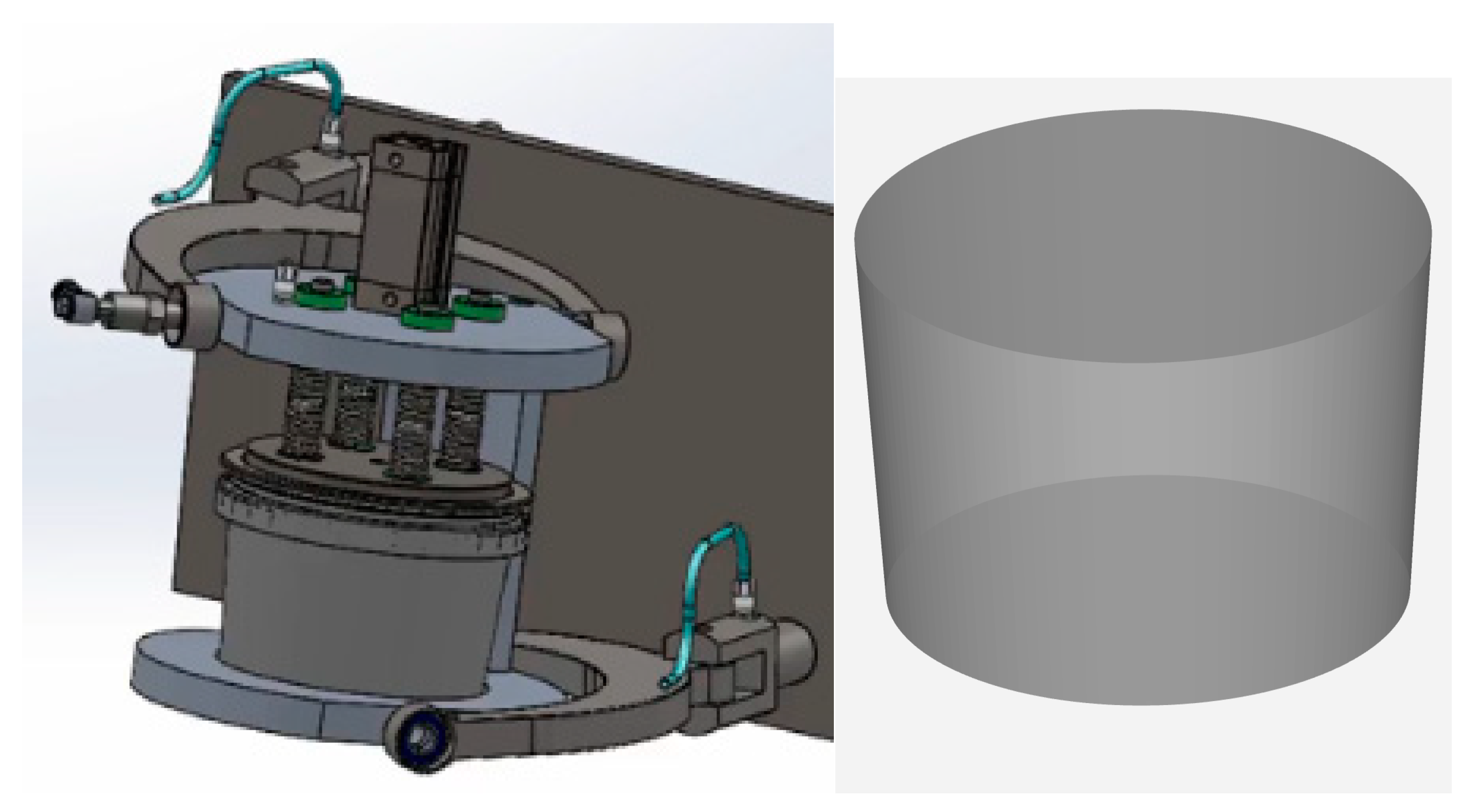
6]. The canister’ volume is 565 mL, but it is filled 70%, it has a trunked cone shape with bottom diameter of 100 mm and top diameter of 118 mm, and a filling height of 76 mm (out of a total canister height of 87 mm). The rotation axis is 76 mm centered below the canister bottom.
The experimental approach was used both to validate the CFD simulation results and to build up the final detergent delivery machine, as the European Research Project requires a high Technical Readiness Level (TRL). The DIY4U objective is to develop a physical prototype which would operate according to the potential end-user requirements (another task of the DIY4U project).
In addition, the project includes the development of a Digital Twin which can provide the mixing results for any combination of detergent component ratios, even if the current detergent components are substituted for by new components. This means that, if the detergent will be produced with different components, the Digital Twin, by merely adjusting the component properties, will yield mixing times of the second detergent mixture without the need of laboratory tests. This is the objective of the development of the Response Surface (RS).
To develop an RS, the whole variable range of detergent parameters should be analyzed. In the present case, the machine rpms are fixed, and the variability occurs only in the percentage of mass fractions of the different detergent components. The application of a quadratic approach to the calculation suggests at least three points per mass fraction component, while subtracting the experiments that would not provide useful information. In sum, RS Model theory calls for 39 cases to be modelled.
The CFD simulations must reproduce the physics of the mixture of the different components that a liquid detergent formula may contain. To allow a proper mixing, with sloshing appearance, the simulations use a partly liquid filled canisters but including an air volume in its upper part. This upper volume includes a second phase, air.
2. Materials and Methods
The simulations were carried out with the CFD solver Fluent v. 2020 version R19 (ANSYS Inc., Canonsburg, PA, USA) [
7] and with the detergent compound data provided by Procter and Gamble (P&G). A simplified detergent formulation was provided by Procter and Gamble, together with key physical property data on the feedstocks.
The CFD simulation has a common procedure starting with the generation of the case geometry model. This model can be observed in
Figure 1.
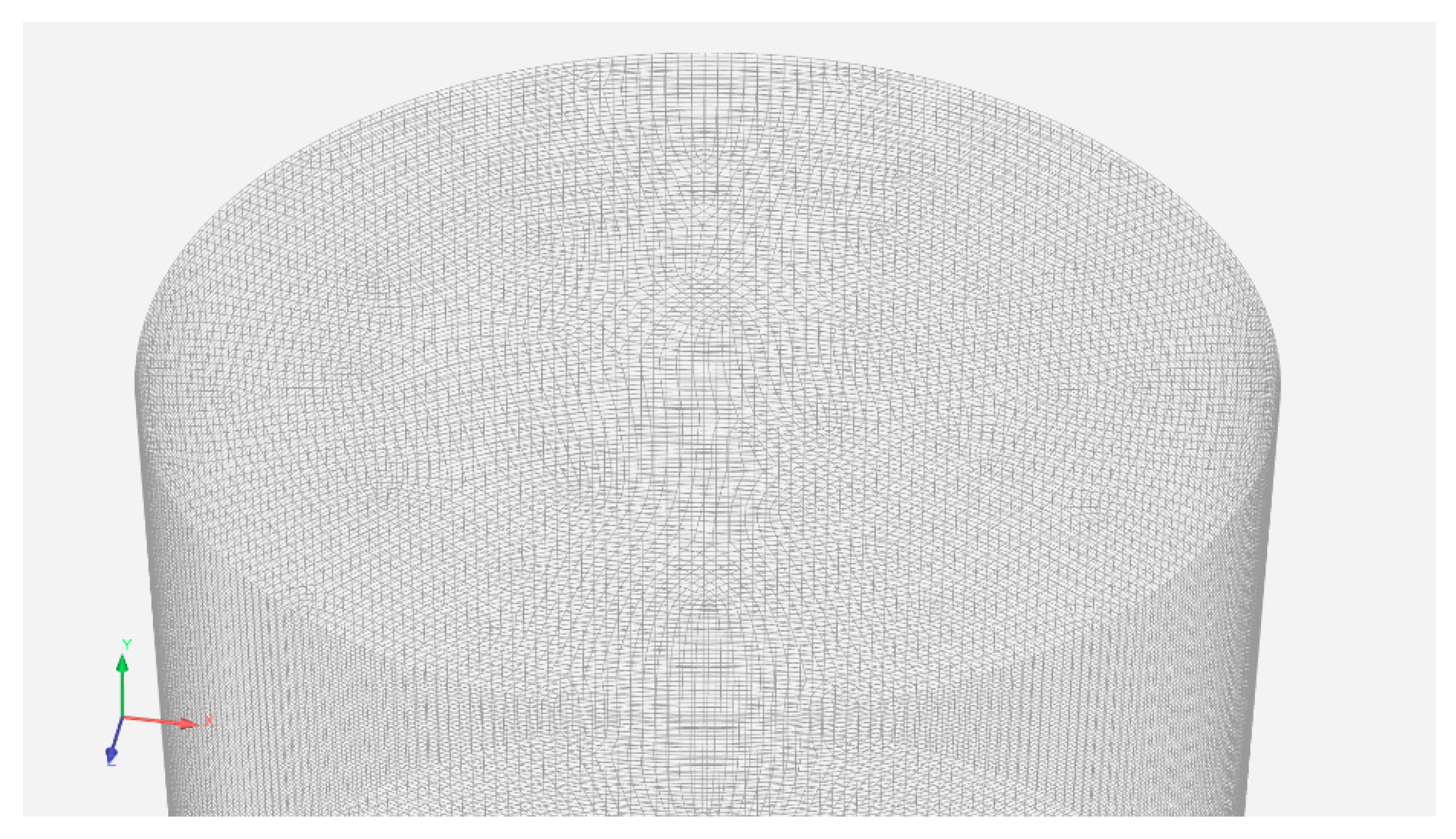
To solve the fluid-dynamics equations or Navier-Stokes equations, the geometry must be divided into small volumes named cells. The group of cells is referred to as the mesh. There are different types of meshes; for the present work, a structured hexahedral mesh was developed. The mesh has 1,925,440 cells, which makes a volume average of 0.3 mm
3/cell. An image of the mesh can be observed in
Figure 2.
Once the mesh has been developed, the materials must be created. As the process is isothermal at normal ambient conditions (25 °C and 1 atm.), heat conductivities and capacities are not required; only the values of density and viscosity are needed.
The compounds’ density and viscosity values can be observed in
Table 1.
Following this, the components are included in the simulation model, and the physics model is defined. The physics model consists of the Navier–Stokes equation for continuity and momentum. No energy equation was required, as the mixing process is isothermal. A turbulence model should be defined as the canister size combined with the turning rpm, creating a turbulent regime. The shear–stress transport model, SST, is chosen, as it models turbulence accurately both in the fluid bulk and near the surfaces where the boundary layer develops.
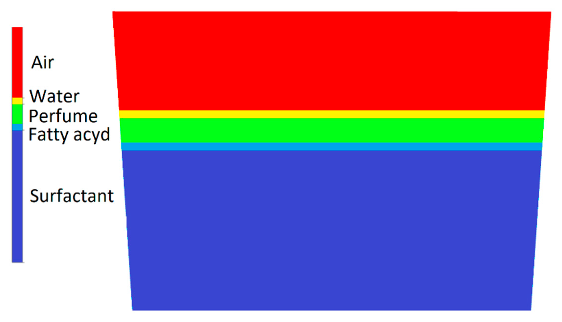
At the initial stage, the canister is steady. The canister is filled by the system by means of ducts pouring each liquid component in the sequence dictated by component storages installed in the mixing equipment, yet under construction. Nevertheless, this process has been replicated in the simulations and performed manually in laboratory, to make both experimental tests and simulations as similar to the final real process as possible. The initial conditions for the simulation define a steady canister, filled with a liquid phase at the bottom and air at the top, with zero velocity, and where the mass fractions of each component in the liquid phase are defined along the height according to the amount dispensed by the system. This is represented in
Figure 3 where the distribution of liquid components at the initial conditions is shown.
Having the physics model defined, the last step is to initialize each case with the different conditions to be considered. The initial conditions are: canister stopped and vertically erected, and the percentages of each component assigned. To develop the mixing process, RS, 39 cases are defined with different component percentages. The summary of such cases can be observed in
Table 2.
Each case was simulated with a transient scheme for several seconds that could be enlarged if, at the end of the initial defined period, the mixing was not complete. Also, due to the high rotating speed, the required time step was set to 0.01 s. Results were saved every 0.25 s to observe the mixing process. Hence, the length of the simulation becomes 10 s with a timestep of 0.025 s (400 iterations).
The computational approach for the CFD model is the following [
7]: the pressure-velocity coupling is defined to coupled. The spatial discretization is defined with the least squares cell based model to calculate the gradients. The pressure is computed with the algorithm PRESTO. The momentum equation is solved with first order upwind discretization, and the volume fraction is calculated with the discretization type compressive (and the implicit formulation [
7]). The mass fractions of the different components were solved with second order upwind. Finally, the transient formulation was first order implicit.
As there was 30% of the volume occupied by air, the mixing quality had to be defined only in the volume occupied by the liquid, which, due to high-speed rotation, showed a high sloshing effect. To calculate the interface between phases and compounds, the Eulerian–mixture multiphase model [
7] is used in the simulations, where the liquid phase is defined as a multicomponent flow. The concentration of each component in the liquid phase is defined by its corresponding mass fraction. All physical properties of the liquid mixture are calculated by the solver as the mass fraction weighted average of the corresponding properties of the individual components. To ensure an accurate representation of the separation between the liquid and gas phases, the sharp–dispersed interphase model [
7] was included. Inside the liquid, the mixing quality was defined as the volume integral of the difference between the local component mass fraction and the expected mass fraction that is the case mass fraction of the regarded compound. This was checked for the five compounds.
The rotation of the canister was defined, implementing a time- and space-dependent gravity vector. The canister rotates around an axis, in the Z-direction and located 76 mm under the canister bottom, and it was adjusted to an equation of simple harmonic movement by making the gravity acceleration components in the rotating plane XY ruled the gravity x-component by the sine function and the y-component by the cosine, hence:
Gravity X component = −9.81 sin (2 PI frequency)
Gravity Y component = −9.81 cos (2 PI frequency)
In this way, instead of the need of working with mesh displacement, the movement was represented by the rotation of the gravity vector around the canister, which has a lower computational cost.
3. Results
Results are individual for each case, where a degree of mixing as function of time was obtained, together with a general mixing process defined with the response surface function, that is, the function which gives the mixing quality as function of time and the compounds percentages.
3.1. Validation
First, some results were required to validate the model. The system was built in the SINTEF lab in Trondheim (Norway), see
Figure 4, and CODY performed one scenario, Scenario 7, at this stage for the liquid detergent mixing. Additional testing will continue prior to the Pilot FABLAB’s being finalized. To perform this scenario, the canister was filled with the same mass fractions as in case 7 of
Table 2, and some photographs were periodically taken to observe the mixing process.
Table 2.
Cases table. Cases are defined by the percentage of each mixture component.
Table 2.
Cases table. Cases are defined by the percentage of each mixture component.
| Case n. | Surfactant Feedstock | Fatty Acid | Dye Solution | Perfume | Water |
|---|
| 1 | 80 | 4 | 6 | 3 | 7 |
| 2 | 80 | 4 | 6 | 0 | 10 |
| 3 | 80 | 4 | 6 | 6 | 4 |
| 4 | 80 | 4 | 0 | 3 | 13 |
| 5 | 80 | 4 | 0 | 6 | 10 |
| 6 | 80 | 4 | 14 | 0 | 2 |
| 7 | 80 | 0 | 6 | 3 | 11 |
| 8 | 80 | 0 | 6 | 6 | 8 |
| 9 | 80 | 0 | 0 | 3 | 17 |
| 10 | 80 | 0 | 0 | 6 | 14 |
| 11 | 80 | 0 | 14 | 0 | 6 |
| 12 | 80 | 12 | 6 | 0 | 2 |
| 13 | 80 | 12 | 0 | 3 | 5 |
| 14 | 80 | 12 | 0 | 0 | 8 |
| 15 | 80 | 12 | 0 | 6 | 2 |
| 16 | 40 | 4 | 6 | 0 | 50 |
| 17 | 40 | 4 | 6 | 6 | 44 |
| 18 | 40 | 4 | 0 | 0 | 56 |
| 19 | 40 | 4 | 0 | 6 | 50 |
| 20 | 40 | 4 | 14 | 3 | 39 |
| 21 | 40 | 4 | 14 | 6 | 36 |
| 22 | 40 | 0 | 6 | 3 | 51 |
| 23 | 40 | 0 | 6 | 0 | 54 |
| 24 | 40 | 0 | 0 | 0 | 60 |
| 25 | 40 | 0 | 14 | 3 | 43 |
| 26 | 40 | 0 | 14 | 0 | 46 |
| 27 | 40 | 12 | 6 | 3 | 39 |
| 28 | 40 | 12 | 6 | 6 | 36 |
| 29 | 40 | 12 | 0 | 6 | 42 |
| 30 | 40 | 12 | 14 | 0 | 34 |
| 31 | 60 | 4 | 6 | 3 | 27 |
| 32 | 60 | 4 | 0 | 0 | 36 |
| 33 | 60 | 4 | 14 | 6 | 16 |
| 34 | 60 | 0 | 6 | 3 | 31 |
| 35 | 60 | 0 | 0 | 0 | 40 |
| 36 | 60 | 0 | 14 | 6 | 20 |
| 37 | 60 | 12 | 6 | 3 | 19 |
| 38 | 60 | 12 | 0 | 0 | 28 |
| 39 | 60 | 12 | 14 | 6 | 8 |
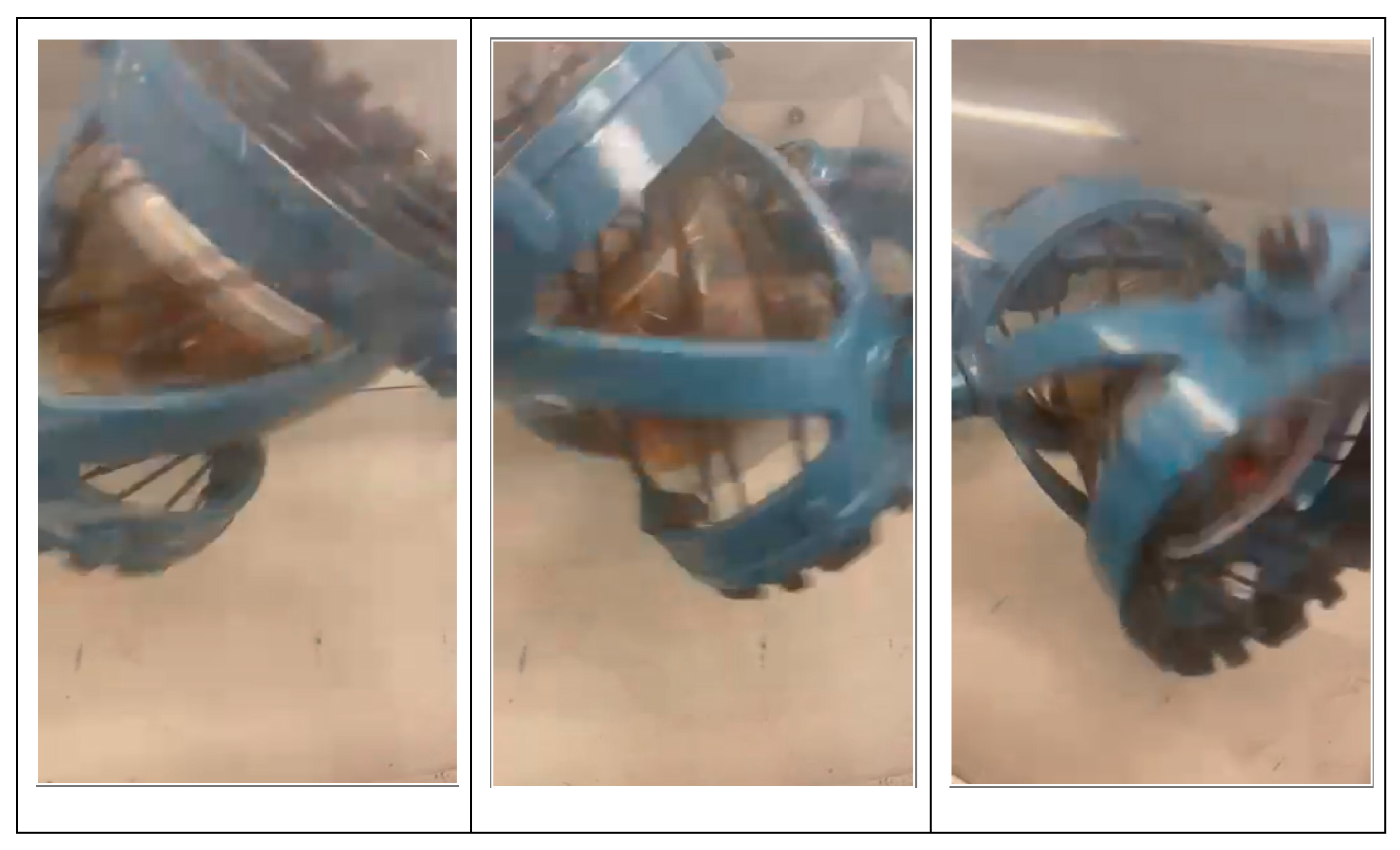
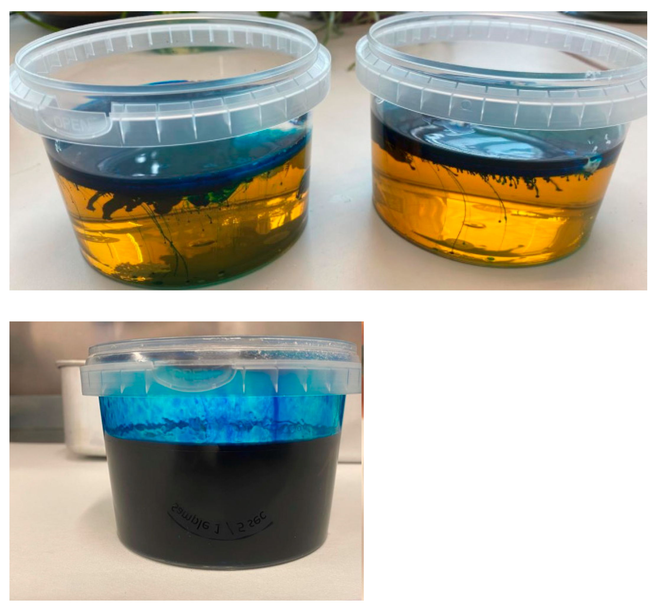
These photographs can be seen in
Figure 5. In this figure, we can observe, in the top picture, the situation before mixing where the surfactant, denser and first added, fills at canister bottom and the dye solution diluted in water, lighter, the top. In the lower picture, the mixed mixture after 7 s. As can be observed, 7 s are appropriate to obtain a good mixture. The experiment corresponding to the validation case was carried out twice to verify reproducibility; the same results were obtained. The photographs of the transparent wall canister at different mixing times of both tests were visually indistinguishable. As each compound has a different color, homogeneity could be visually observed
The same process was carried out for other cases, but no substantial differences were observed. For that reason, other results are not included here.
3.2. Cases Results
This section shows the results of one case in two ways: first, qualitative results, images of the mixture process where, with colored maps could be seen the already mixed zones and those where the average mass fraction is still not at the fed value; secondly, there will be shown the mixing quality function as a quantitative result.
3.2.1. Qualitative Results
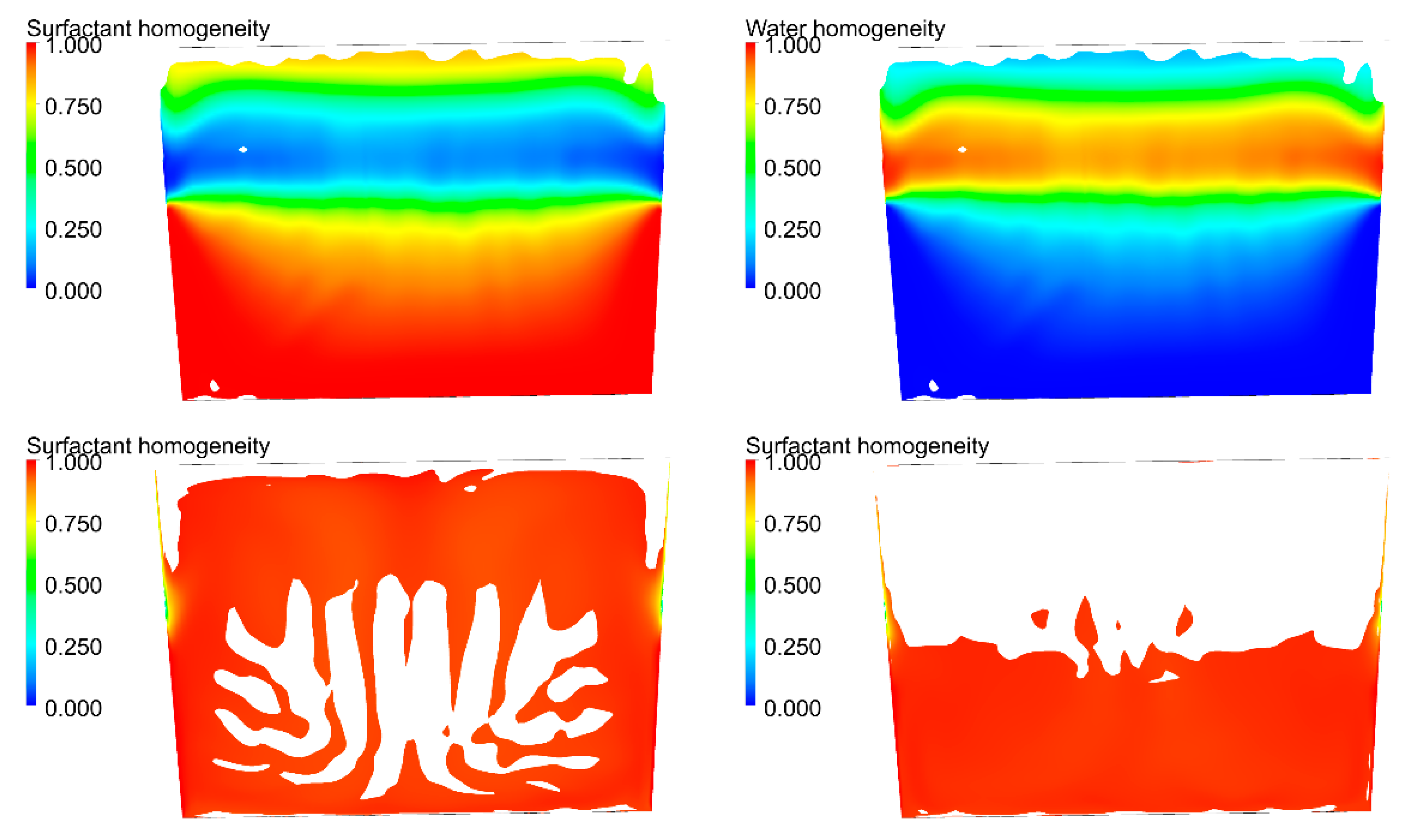
The mixing process can be observed in the following images for case 7, used as model validation.
Figure 4 shows the surfactant feedstock concentration after 0.25 s of mixing. The surfactant was fed at the canister bottom and most of it has still not moved.
Only a part of the surfactant, the part with lower concentration, has been moved to the canister top due to its rotation and is falling. This part is, logically, with lower concentration, as it has mixed with the other components. Finally, the dark blue zone corresponds to the air-filled zone.
Figure 6 show the homogenization progress, finally achieved at around 7.5 s. The final mixture time is very near to that recorded in the lab experiments. It assures the validation of the simulation model. Then, we proceed with all the additional cases to be simulated. The results of the additional scenarios are shown only numerically in the next section, as qualitative results do not provide further process insight compared to what has already been described.
3.2.2. Quantitative Results
Once, all the scenarios have been calculated, maintaining a good convergence for all of them, the homogeneity equation (to be included in the Digital Twin of the DIY4U project) was defined as: one minus the sum, for all the detergent components, of the mass fraction maximum value in the volume minus the mass fraction minimum value, divided by the expected average mass fraction value (that of the amount fed into the canister). Then, when homogeneity is far from being reached, the homogeneity function is near zero. Alternatively, homogeneity is achieved when it reaches the value of 1. Hence, the equation has the form:
The values of homogeneity function as function of time for each case can be observed in
Table 3.
Finally, mixing time results are quite similar for all the cases. These mixing results are included in a single equation of homogeneity depending on both the time and the mass fraction of the different compounds. For future compounds the mixing time could differ much more. The developed equation has the expression:
where:
hf: is the homogeneity factor, being 0 for completely separated compounds and 1 for fully mixed.
surf.mf: is the surfactant mass fraction.
fa.mf: is the fatty acid mass fraction.
ds.mf: is the dye solution mass fraction.
perf.mf: is the perfume mass fraction.
w.mf: is the water mass fraction.
t: is time in seconds.
In cases where a mass fraction is zero, it must be regarded as a very small value, such as 0.00001.
With the values for this equation, times, mass fractions and simulation values, an uncertainty study was carried out, obtaining a mean absolute error of 0.028 and a mean quadratic deviation of 0.0006.
4. Conclusions
The main conclusion for the study is that the agitation of a mixing system using an exocentric rotation axis at a quite high rotation speed, 45 rpm, produces a fast mixing which takes less than 10 s for any combination of detergent components to be properly mixed.
CFD simulations and the obtained response surface formulation developed from the 39 scenarios are a good method to define a digital tool which would allow the analysis of any formulation by merely adjusting the component properties, avoiding the use of material, and saving lab testing time and money.
Author Contributions
Conceptualization, J.D., A.I., A.K.S., M.G. and J.H.; methodology, J.D. and A.I.; software, J.D., A.I. and D.A.; validation, J.D., A.I., D.A. and J.H.; formal analysis, J.D. and A.I.; investigation, J.D. and A.I.; resources, M.G. and J.H.; data curation, J.D., A.I., M.G. and J.H.; writing—original draft preparation, J.D.; writing—review and editing, J.D. and A.I.; visualization, D.A.; supervision, A.K.S.; project administration, A.K.S. and M.G.; funding acquisition, A.K.S. All authors have read and agreed to the published version of the manuscript.
Funding
This research was funded by European Union´s Horizon 2020 research and innovation programme, project DIY4U grant number GA No. 870148. The APC was funded by European Union, project DIY4U grant number GA No. 870148.
Acknowledgments
The DIY4U project has received funding from the European Union’s Horizon 2020 research and innovation programme under GA No. 870148.
Conflicts of Interest
The authors declare no conflict of interest.
References
- Mayer, C.; Gatumel, C.; Berthiaux, H. Scale-up in Turbula© mixers based on the principle of similarities. Part. Sci. Tech. 2020, 38, 973–984. [Google Scholar] [CrossRef]
- Mayer, C.; Gatumel, C.; Berthiaux, H. Mixing dynamics for easy flowing powders in a lab-scale Turbula© mixer. Chem. Eng. Res. Des. 2014, 95, 248–261. [Google Scholar] [CrossRef]
- Coulaloglou, C.A.; Tavlarides, L.L. Description of interaction processes in agitated liquid-liquid dispersions. Chem. Eng. Sci. 1977, 32, 1289–1297. [Google Scholar] [CrossRef]
- Edwards, M.F.; Baker, M.R. A review of liquid mixing equipment. In Mixing in the Process Industries, 2nd ed.; Butterworth-Hienemann: Oxford, UK, 1997; Chapter 7; pp. 118–136. [Google Scholar]
- Ghotli, R.A.; Raman, A.A.A.; Ibrahim, S.; Baroutian, S. Liquid-liquid mixing in stirred vessels: A review. Chem. Eng. Commun. 2013, 200, 595–627. [Google Scholar] [CrossRef]
- Nere, N.K.; Patwardham, A.W.; Joshi, J.B. Liquid-phase mixing in stirred vessels: Turbulent flow regime. Ind. Eng. Chem. Res. 2003, 42, 2661–2698. [Google Scholar] [CrossRef]
- ANSYS Inc. Fluent R19 Documentation; ANSYS Inc.: Canonsburg, PA, USA, 2019. [Google Scholar]
| Disclaimer/Publisher’s Note: The statements, opinions and data contained in all publications are solely those of the individual author(s) and contributor(s) and not of MDPI and/or the editor(s). MDPI and/or the editor(s) disclaim responsibility for any injury to people or property resulting from any ideas, methods, instructions or products referred to in the content. |
© 2022 by the authors. Licensee MDPI, Basel, Switzerland. This article is an open access article distributed under the terms and conditions of the Creative Commons Attribution (CC BY) license (https://creativecommons.org/licenses/by/4.0/).


 ,
, 


