Abstract
In a wind tunnel process, Mach number is the most important parameter. However, it is difficult to measure directly, especially in the multimode operation process, leading to difficulty in process monitoring. Thus, it is necessary to measure the Mach number indirectly by utilizing data-driven methods, and based on which, to monitor the operation status of the wind tunnel process. In this paper, therefore, a multimode wind tunnel flow field system monitoring strategy is proposed. Since the wind tunnel system is a strongly nonlinear system, the kernel partial least squares method, which can efficiently handle the nonlinear regression problem, is utilized. Firstly, the Mach number is predicted utilizing the kernel partial least squares method. Secondly, process monitoring statistics, i.e., the Hotelling T2 statistic and the square prediction error, the SPE statistic, and their control limits, are proposed to be applied to monitor the wind tunnel process on the basis of the prediction of the Mach number. Finally, the Mach number prediction and monitoring strategy are applied to a real process, where mode analysis and division is necessary. After mode division, the single-mode and multimode processes are modeled and predicted, respectively, and both the single-mode and multimode processes are monitored online. Satisfactory results were achieved compared with those of the partial least squares method.
1. Introduction
In wind tunnel systems, power devices are used to drive controllable air flow through an annular pipe to conduct various aerodynamic tests [1]. Additionally, the wind tunnel systems contribute significantly to the space industry [2]. Since aerospace vehicles develop rapidly, the number of wind tunnel tests has increased greatly. Because the wind tunnel system is an extremely complex, multivariable, nonlinear system with multiple working conditions and multiple correlations between variables, determining how to develop a wind tunnel system model suitable for multiple working conditions is difficult. The most critical factor in modeling each condition of the wind tunnel system is the need to collect a lot of data to ensure accuracy. It needs many test times to obtain high precision in the model during the wind tunnel operation and testing, and each time the test energy consumption is very high; thus, the wind tunnel test would be improved if a safe operation process can be guaranteed and less data were necessary to guarantee the accuracy of the model. In recent years, with the improvement in wind tunnel equipment, wind tunnels undergo more and more test tasks. The tests are increasingly difficult, and the demand for safety and stable operation is greater [3]. Therefore, in the operation of a wind tunnel, it is particularly important to monitor the operation state of the process, and it is of great significance to frequently check the abnormal system operation for the operation of the wind tunnel. In addition, complex working conditions and high energy consumption also make it very important to analyze and model for multiple working conditions, capturing the relationship between multiple modes, and evaluating the efficiency of building models for multiple working conditions.
Although the Mach number is very important in the wind tunnel flow field, it is usually not easy to acquire directly using mechanical principles, especially for multiple working modes. Therefore, it is typical to predict the Mach number through soft measurements. Several researchers recently proposed methodologies for Mach number predictions. For example, Wang et al. predicted the Mach number of a wind tunnel based on the random forest method [4]; Du et al. established an integrated neural network on the basis of a feature subset to predict the Mach number [5]; Guo et al. developed a time slice model, using the partial least squares (PLS) method in multimode wind tunnel systems [6]; and Yuan Ping et al. developed a kernel partial least squares (KPLS) Mach number prediction strategy focusing on the nonlinear characteristic of the wind tunnel system [7]. In their work, the KPLS method was applied to build time slice models and mean value models. As stated above, prediction methods for the Mach number have been investigated and the Mach number prediction problem has been solved to a certain degree. However, few works have been conducted about wind tunnel system monitoring based on the Mach number predictions, thus, how to utilize the online Mach number predictions to monitor the wind tunnel flow field is still a problem which has to be settled urgently.
The KPLS method was proposed based on the PLS method. In 1980s, PLS was first proposed to capture the relationship between independent and dependent variables [8]. Since then, PLS was applied widely in the fields of statistical modeling, monitoring, and quality prediction and control [9,10,11,12], especially for batch processes [13,14,15]. Afterwards, a kernel function was introduced into PLS to handle the nonlinear problem [16,17,18,19]. Therefore, it can be used to solve the nonlinear regression problem for industrial processes where process data usually exhibit strong nonlinearity.
In this paper, a strategy for Mach number monitoring on the basis of Mach number prediction, which considers the nonlinear characteristic and the multimode characteristic in a wind tunnel system, is proposed. Considering that the models built based on the process variables stored in time slices are very easily affected by noise and the predictions may fluctuate heavily, the mean matrices of the variable time slices are preferred to build the regression model. Thus, the KPLS algorithm is applied to establish the relationship between the mean matrix of the process variables and the Mach number of the time slices within each working mode. In addition, the statistical indexes, i.e., the Hotelling T2 statistic and the square prediction error, SPE statistic, and their control limits, are proposed for the Mach number monitoring based on the KPLS method. Consequently, the Mach number prediction and monitoring strategies are applied to a real process, where mode analysis and division is necessary. Through mode analysis based on process knowledge, the concerned multiple working conditions are divided into several modes. After mode division, the single-mode and multimode processes are modeled and predicted, respectively, and both are monitored online. The Mach number prediction results as well as the monitoring results for each mode are compared with those from the PLS method. In addition, a multimode prediction and monitoring analysis is accomplished adopting the proposed prediction and monitoring strategy, of which the results are also compared with those obtained by the PLS method. Finally, a faulty process is monitored and identified.
The following sections of this paper include the following: in Section 2, the mean matrix KPLS model is introduced, as well as the according monitoring strategy based on KPLS. Section 3 begins with the structure of the wind tunnel, and then the proposed Mach number monitoring strategies are illustrated for the multiple modes in detail, compared with the mean matrix PLS models. Additionally, a faulty process is monitored and identified. Finally, in Section 4, the conclusions are presented.
2. Methodology
2.1. Mean Matrix KPLS Regression Model
To deal with the multiple working conditions, the collected data are stored in a way similar to batch processes, that is, each test of the wind tunnel process is considered as a batch, and the data are stored in a two-dimensional matrix with the variable direction and the time direction. Data of several tests with the same working conditions constitute a data block, which is a three-dimensional matrix, adding the test direction as the third direction. Furthermore, some data blocks from neighboring working conditions will form the data matrix of one working mode by analyzing process knowledge, which is still a three-dimensional matrix. The details of mode division will be outlined in the simulation section. Here, the methodology will be focused on for each mode. That is, the methodology comprises the modeling and monitoring strategies for one mode.
As stated above, in each working mode, the measured process variable data forms a three-dimensional data matrix, , where I represents the total number of tests, represents the total number of process variables, and K represents the total number of sample times within each test. The measured dependent variable of I tests are stored in the matrix . After normalization, the normalized process variable and the quality variable are denoted as and . Then, by decomposing the normalized process variable data matrix, , along the time axis, K time slice matrices can be obtained, i.e., , . Similarly, by decomposing the normalized quality variable data matrix, , along the time axis, K time slice matrices can be obtained, i.e., .
The KPLS method is introduced to solve the nonlinear problem [20]. First, process data are projected nonlinearly by the mapping function,
where x is a vector in the initial space, is the n-dimensional Euclidean space, is the constructed mapping function, and the high-dimensional feature space. The appropriate kernel function should be selected to accomplish the mapping. The inner product in the feature space is
where z is a vector in the initial space. There are many kernel function forms, and usually, it is necessary to carefully choose the kernel function to better transform the characteristics of the process variables. Common kernel functions include the Gaussian kernel function, the polynomial kernel function, the radial kernel function, exponential kernel function, and so on. Typically, the Gaussian kernel function can be expressed as
The polynomial kernel function can be expressed as
For concision, only these two typical kernel functions are introduced here.
In a previous work, heavy noise in the time slice models was found, and the mean value model, which is built based on the parameters of the time slice models, was proven to produce better prediction results than the time slice models [7]. However, usually, there may be thousands of time slice models, and the kernel transformation of each time slice variable matrix to obtain the regression parameters of KPLS may take a long time, which is not efficient. Therefore, a novel way to build the model, i.e., the mean matrix model based on the time slice models, is proposed here. The mean value process variable matrix is obtained before the kernel transformation, and only needs to conduct the kernel transformation once on the mean value process variable matrix to acquire the regression parameter of the mean matrix model. The details are introduced below.
To avoid the influence of noise, the mean value of the process data and the mean value of the quality data of each mode during the certain time period are first obtained before conducting the kernel transformation, as follows:
Then, the mean value of the process data matrix, , is projected into the selected high dimensional kernel space, obtaining the data matrix denoted as .
In this high dimensional space, and can be treated in a linear way. Thus, the mean matrix PLS model can be obtained as follows [16,21]:
where and U are the score matrices, and are the loading matrix and loading vectors, E and are the residual matrix and residual vectors.
A typical NIPALS-KPLS algorithm is shown below.
- Initialize u randomly.
- .
- .
- .
- Repeat steps 2–5 until convergence.
- .
- Return to 2, until all latent variables are calculated.
The regression relationship between and can be written directly as
where is the regression parameter vector.
For the new process data that need to be predicted after the kernel transformation, , the quality prediction is
2.2. Mach Number Monitoring Based on KPLS
In this paper, online monitoring is conducted based on the Hotelling T2 statistic and the square prediction error (SPE) statistic. The Hotelling T2 statistic measures the process variation of the principal space, represented by the deviation of latent variables. SPE statistic measures the process variation of the residual space, representing by the deviation of the process variables.
In the current operating condition, the definitions of the Hotelling T2 statistic and the SPE statistic are
where is the residual vector at the k-th moment.
Their control limits are
where is the F distribution with the confidence and degrees of freedom, and , and is the total number of retained latent variables; is the distribution with the confidence level of and the proportional coefficient of ; ; is the mean value of SPEk; and is the variance of SPEk, k = 1,…,K.
For the new process variable vector , which needs to be monitored, the online statistics are calculated as
where is the residual vector at the k-th moment.
3. Illustration and Discussion
3.1. Wind Tunnel System
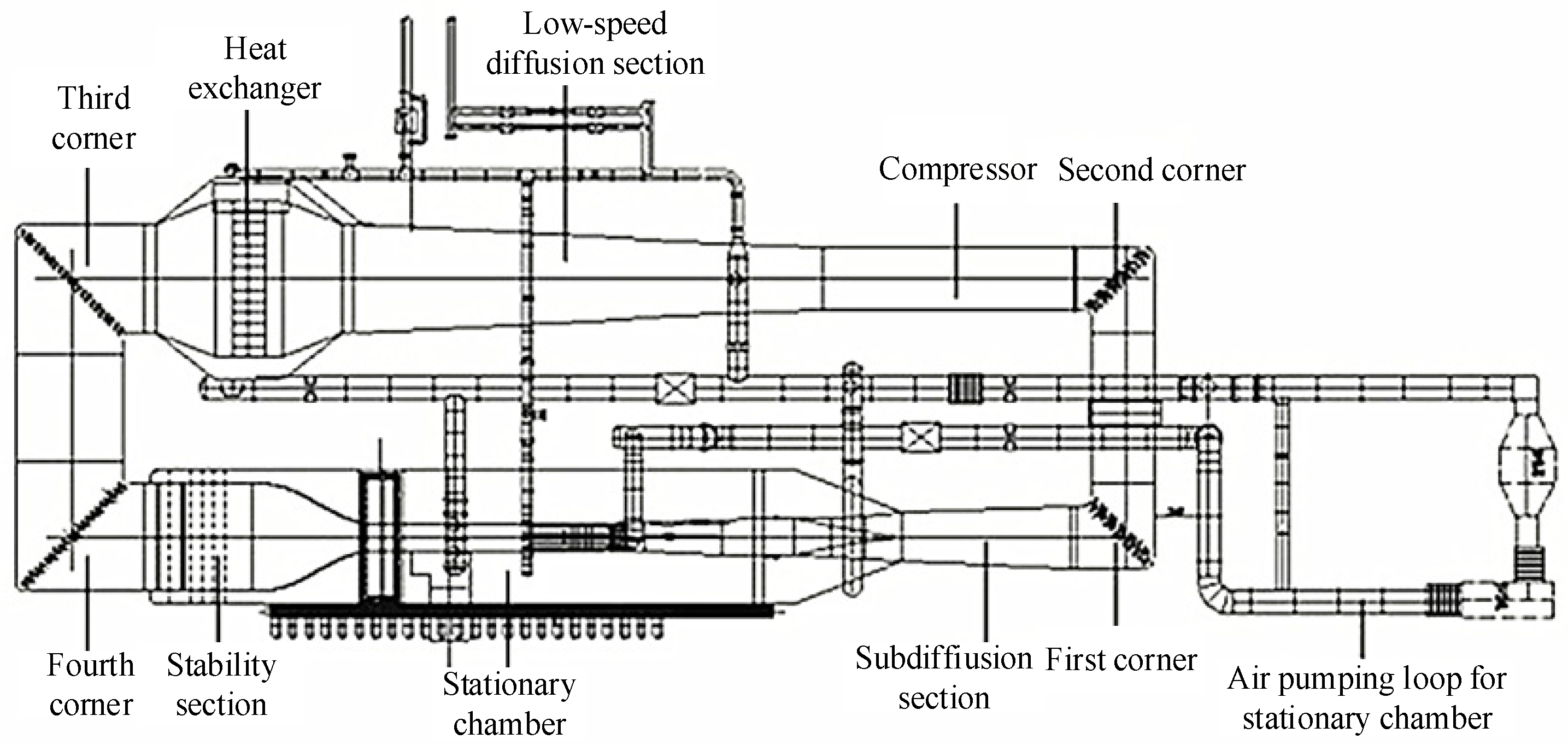
Figure 1 shows a typical continuous transonic wind tunnel, which is a Chinese low-noise variable density reverse channel built in 2012. The wind tunnel investigated in this work is 0.6 m × 0.6 m. The design scheme of the wind tunnel adopts the compressor drive system with wide working condition and its integration with the wind tunnel, semi-flexible wall nozzle, low-noise transonic test section, main injection slot of fingerboard re-entry regulator, high-performance heat exchanger, and three-stage regulator, plus an adjustable central throat and other new technologies.
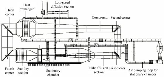
Figure 1.
Structure of a wind tunnel system.
When the wind tunnel starts working, the wind tunnel flow field is quickly formed. After a period of operation in the wind tunnel, the gas continuously enters the tunnel. Through controlling the main exhaust valve to empty the gas, the total air pressure in the stability section and the static pressure of the test segment will reach the target value, thus the Mach number will be stable.
There are a great deal of working conditions associated with a wind tunnel process due to varying parameter settings. Many process parameters exist in a wind tunnel process, such as jet groove, opening/closing ratio, and control mode of the total pressure, while their influences on the working condition division are not quite clear. In addition, it is not sensible to build models for each working condition with any slight change in any process parameter. Therefore, how to conduct meaningful mode division is significant for the wind tunnel system. After careful analysis of the knowledge of the wind tunnel process, the working condition with the J7 model, 28 mm jet groove, an opening and closing ratio of 2%, and the negative pressure mode are investigated in this paper. Within one working condition, there are still many other operation factors, such as the attack angle step, the speed setting value, and so on, which will have a large influence on the mode division, and further affect the modeling of the Mach number. The concerned process variables are listed in Table 1. Due to the fact that, in the specific wind tunnel process, the motor speed of 1800 rpm is a typical working condition, here, the 1800 r motor speed is applied. Additionally, the influence of the attack angle change to the wind tunnel field is of interesting to researchers in this field; thus, the attack angle steps are used as the index to divide the data block into different working modes, which are shown in Table 2. The attack angle step of Mode 1 is 2, which includes data blocks 1, 2, 3, and 4, and the attack angle step of Mode 2 is 1, which includes data blocks 5, 6, 7, 8, and 9. Each data block stores the process data under the same working condition.

Table 1.
Process variables.
Table 2.
Operating modes.
The following simulation will be accomplished based on these two data modes with different data blocks. In Mode 1, some of the data of block 3 are taken as the test data, and the rest of the data in Mode 1 are taken as the training data. For convenience, the test data and training data for mode 1 are called test data 1 and training data 1, respectively. The dimensions of training data 1 are 4 × 20 × 654, and the dimensions of test data 1 are 1 × 20 × 654. Similarly, in Mode 2, some of the data of block 7 are taken as the test data, and the rest of the data in Mode 2 are taken as the training data, which are called test data 2 and training data 2, respectively. The dimensions of training data 2 are 5 × 20 × 654, and the dimensions of test data 2 are 1 × 20 × 654. For multimode analysis, training data 1 and training data 2 are combined to form the training data of the multiple modes, with the dimensions 8 × 20 × 654. Moreover, test data 1 and test data 2 are still used in the test, representing Mode 1 and Mode 2, respectively.
3.2. Mach Number Prediction Based on KPLS Model
In this section, firstly, to verify the prediction precision, mean matrix KPLS models are built for single modes, Mode 1 and Mode 2, respectively, and the predictions of the mean matrix KPLS model as well as the predictions of the mean matrix PLS model are obtained and compared. Secondly, the multiple modes, which consist of Mode 1 and Mode 2, are used as the object to conduct the multimode Mach number prediction to illustrate the effectiveness of the prediction strategy based on mode division.
- A.
- Single-mode prediction
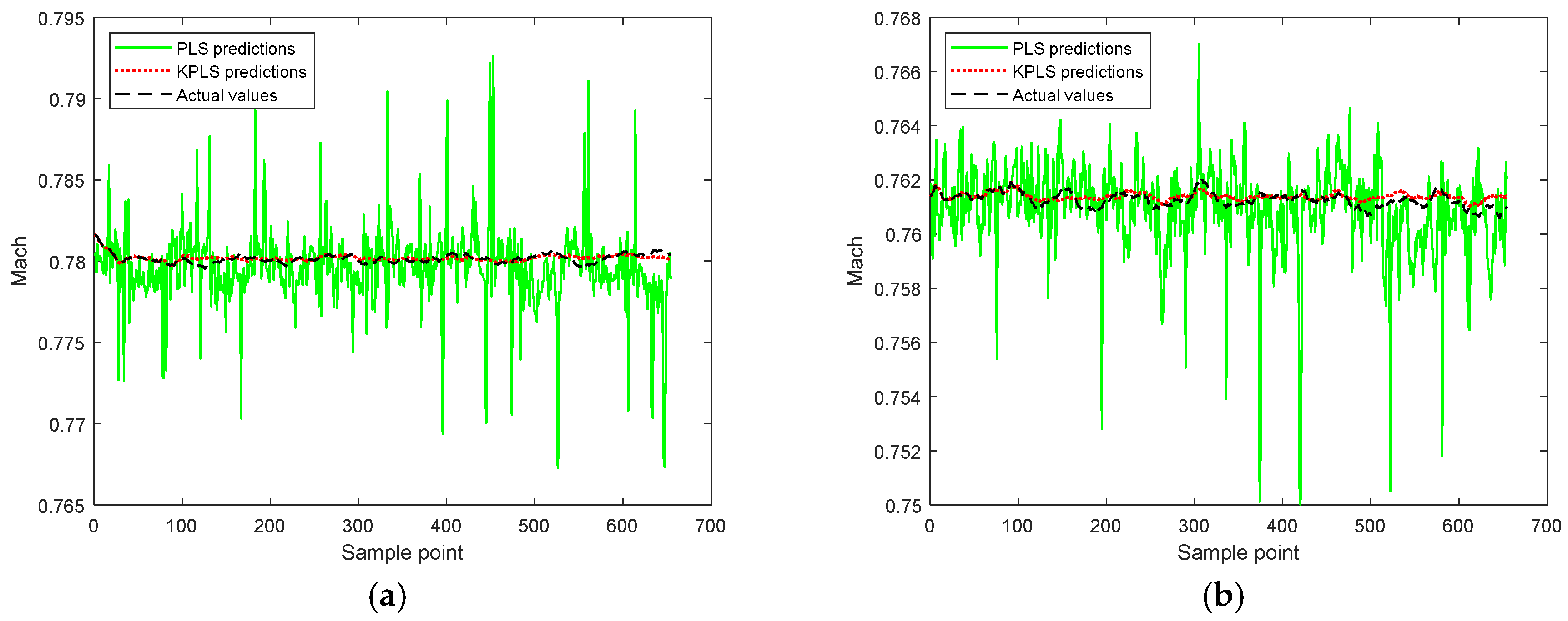
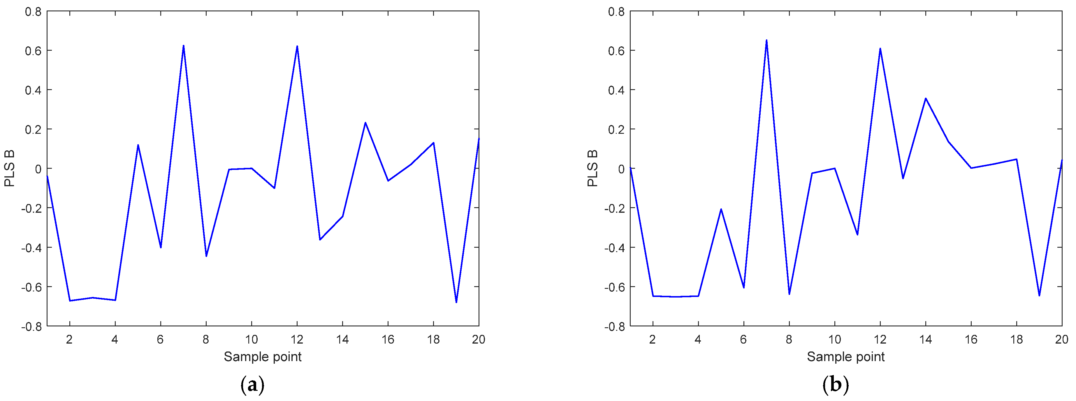
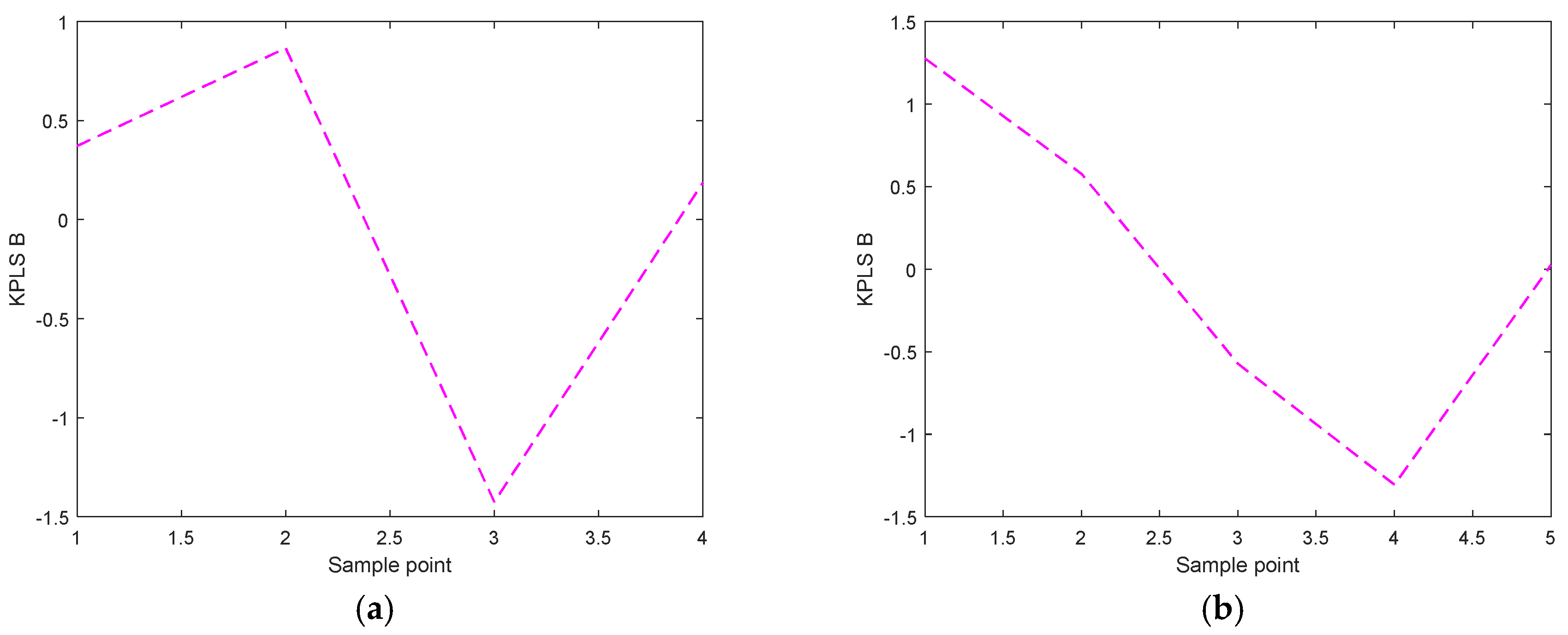
Firstly, mean matrix KPLS models and mean matrix PLS models are built utilizing the training data and the test data of each mode. The prediction results of Mode 1 and Mode 2 are shown in Figure 2a,b, respectively. It can be seen that better prediction results are provided by the mean matrix KPLS model than the mean matrix PLS model. Obviously, the prediction results of the mean matrix KPLS model are much closer to the actual values of the Mach number, and there are many fluctuations in the predictions results of the mean matrix PLS model, which are caused by the unmodeled dynamics and processes that are not taken into account in the PLS method assumptions. The regression parameters of the mean matrix PLS model and the mean matrix KPLS model are shown in Figure 3 and Figure 4. From Figure 3, it can be seen that process variables 2, 3, 4, 12, 17, and 19, which are stable static pressure, test static pressure, outlet static pressure, main inlet pressure, auxiliary output temperature, and mass flow of the auxiliary inlet, respectively, have larger impacts on the predicted variables than the others. From Figure 4, the regression parameter of KPLS does not reflect the regression relationship with the process variables due to the kernel matrix.
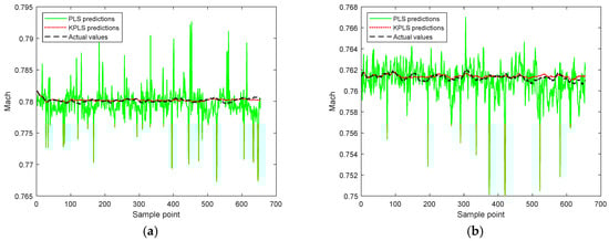
Figure 2.
Mach number prediction results: (a) Mode 1; (b) Mode 2.
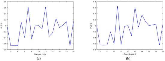
Figure 3.
PLS regression parameter: (a) Mode 1; (b) Mode 2.
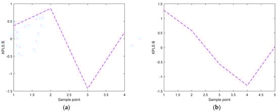
Figure 4.
KPLS regression parameter: (a) Mode 1; (b) Mode 2.
- B.
- Multimode prediction
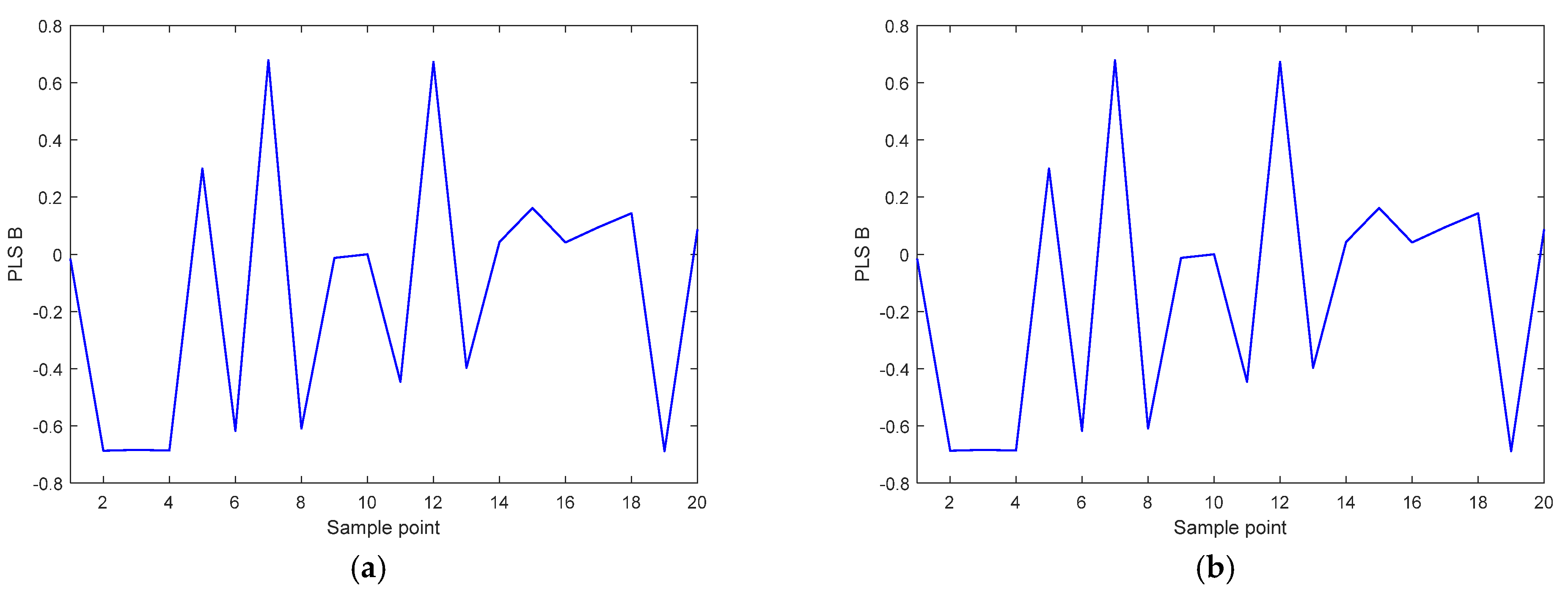
After the analysis for single modes, multiple modes, which consist of Mode 1 and Mode 2, are focused on. That is, training data 1 and training data 2 are combined to form the training data of the multiple modes. The multimode prediction can help to judge whether it is necessary to model each mode respectively. Firstly, using the combined training data of the two modes, the mean matrix KPLS model and the mean matrix PLS model are built. Test data 1 and test data 2 are predicted, respectively, to clearly observe the prediction results for each mode. The prediction results are represented in Figure 5a,b. It can be seen that the mean matrix KPLS model provides much better predictions than the mean matrix PLS model. Similar to the single-mode prediction, the predictions of the mean matrix KPLS model are much closer to the actual values of the Mach number, and there are many fluctuations in the predictions of the mean matrix PLS model. The regression parameters of the mean matrix PLS model and the mean matrix KPLS model are shown in Figure 6 and Figure 7. From Figure 6, it can be seen that the regression parameters for Mode 1 and Mode 2 are the same, which conforms to the modeling strategy. Additionally, they are similar to the regression parameters obtained by for the single modes.
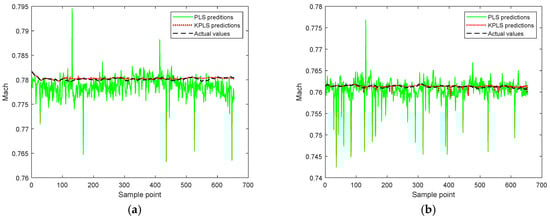
Figure 5.
Multimode Mach number prediction results of the mean matrix PLS and mean matrix KPLS models: (a) test data 1; (b) test data 2.
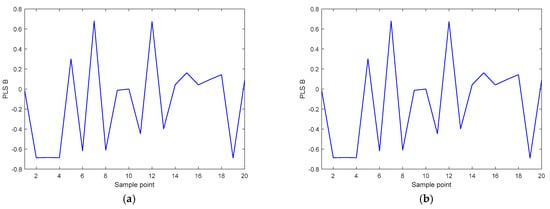
Figure 6.
PLS regression parameter: (a) Mode 1; (b) Mode 2.
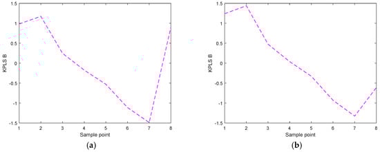
Figure 7.
KPLS regression parameter: (a) Mode 1; (b) Mode 2.
The RMSE values of each mode and multimode predictions were calculated and are shown in Table 3. Since the RMSE values of the mean matrix PLS model are approximately ten times of those of the mean matrix KPLS model, it can be concluded that the mean matrix KPLS model is better than the mean matrix PLS model. This is consistent with the anticipation that since the wind tunnel field has strong nonlinear characteristics, the KPLS model, which can handle the nonlinear regression problem, would provide better prediction results than the PLS model, which deals with linear regression. Meanwhile, the RMSE values of the predictions of the KPLS model satisfy the prediction precision, and the prediction results of the single-mode model are better than those of the multimode model. This means that if these data blocks were combined as one mode, i.e., without dividing into two modes, the prediction results will be worse. Thus, mode division is necessary for the wind tunnel flow field system, and, based on good mode division, modeling for each mode will be more efficient. The standard deviations of PLS and KPLS are listed below in Table 4 [22]. The standard deviations of the regression parameters of the mean matrix PLS model are around 0.4, while those of the mean matrix KPLS model are around 0.99.
Table 3.
RMSE values of predictions.
Table 4.
Standard deviations of the regression parameters.
As shown above, the Mach number predictions satisfy the required precision. This proves that the relationship captured by the mean matrix KPLS model strongly represents the real relationship between the process variables and the Mach number. Since the mean matrix KPLS model provides better predictions than the mean matrix PLS model, the relationship captured by the mean matrix KPLS is more reliable than the mean matrix PLS model. Moreover, it can be implied that the following monitoring based on the mean matrix KPLS model would be more reliable than that based on the mean matrix PLS model. This implication illustrates that the Mach number prediction is an indispensable step before applying the specific monitoring strategy. Obviously, if a mode cannot accurately represent the relationship between variables, the monitoring strategy based on this model also cannot monitor the process correctly.
3.3. Mach Number Monitoring
In this section, firstly, based on the mean matrix KPLS models, the monitoring statistics as well as their control limits are calculated for the normal test data of Mode 1 and Mode 2, respectively. Secondly, the multimode Mach number monitoring process is conducted. Finally, a faulty process is monitored.
- A.
- Single-mode monitoring
Firstly, the T2 and SPE statistics and their statistical control limits are calculated for each mode based on the quality prediction for single modes. The confidence level α is set to 0.9. The monitoring results of normal data of Mode 1 and Mode 2 are obtained, and are shown in Figure 8a,b,c,d, respectively. In these figures, both the T2 and SPE statistics are beneath their control limits, which means the test data are in a normal status. Therefore, the mean matrix KPLS model provides satisfactory monitoring results.
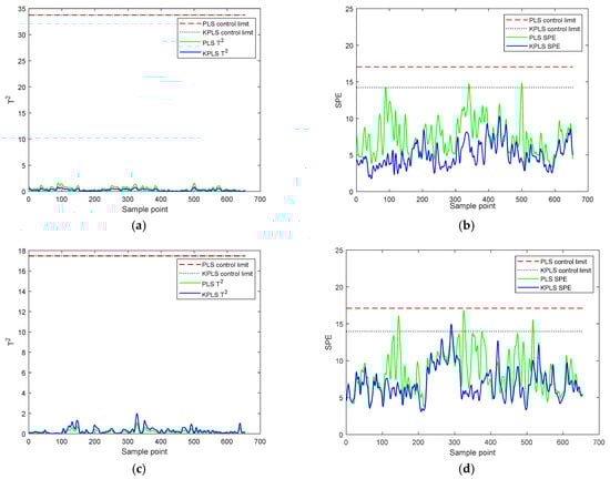
Figure 8.
Mach number monitoring results: (a) T2 for Mode 1; (b) SPE for Mode 1; (c) T2 for Mode 2; (d) SPE for Mode 2.
- B.
- Multimode monitoring
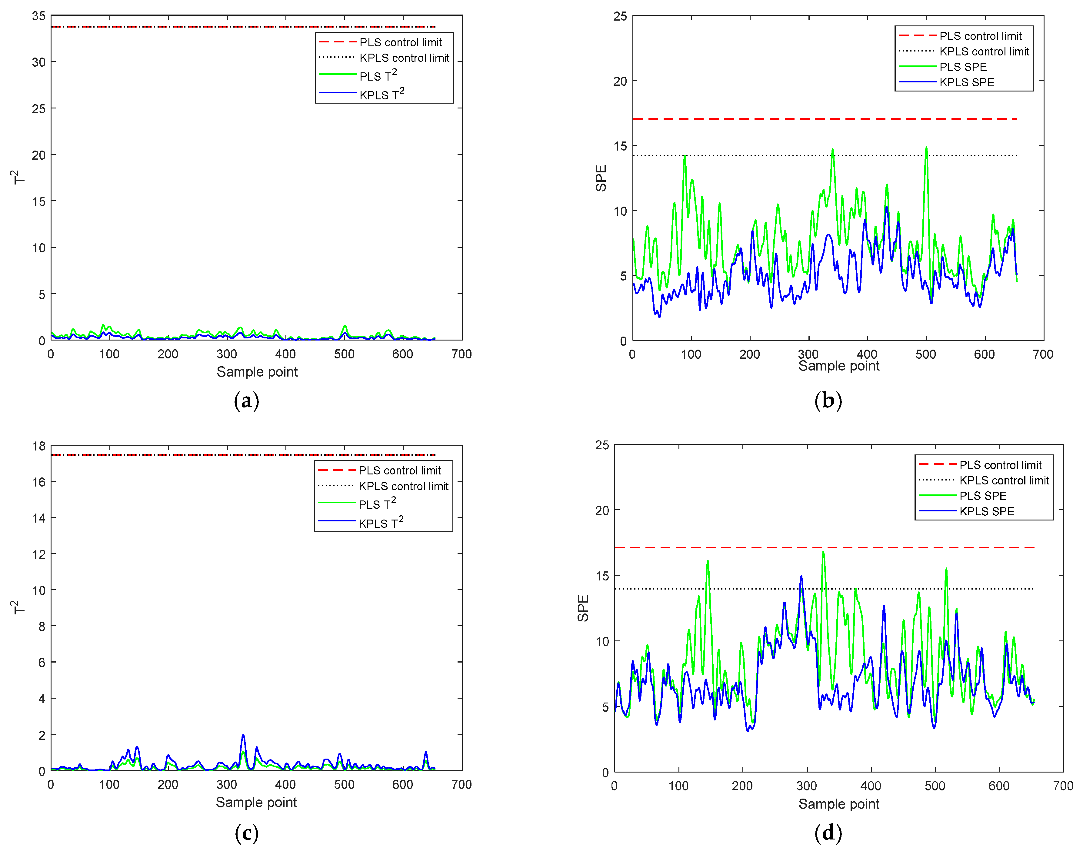
Afterwards, normal test data 1 and test data 2 are monitored. The T2 and SPE statistics and their statistical control limits are accordingly calculated based on the quality prediction for multiple modes. The monitoring results are represented in Figure 9a–d. Both the T2 and SPE statistics of the mean matrix KPLS model are beneath the control limits, which means the test data are in a normal status. Meanwhile, some points of the SPE statistic of the mean matrix PLS model go beyond the control limits. In addition, the monitoring results of the mean matrix KPLS model are more satisfactory than those of the mean matrix PLS model, since there is some noise in SPE that exceeds the controls limits and may cause false alarms.
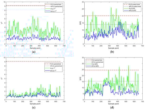
Figure 9.
Multimode Mach number monitoring results: (a) T2 for test data 1; (b) SPE for test data 1; (c) T2 for test data 2; (d) SPE for test data 2.
- C.
- Fault monitoring
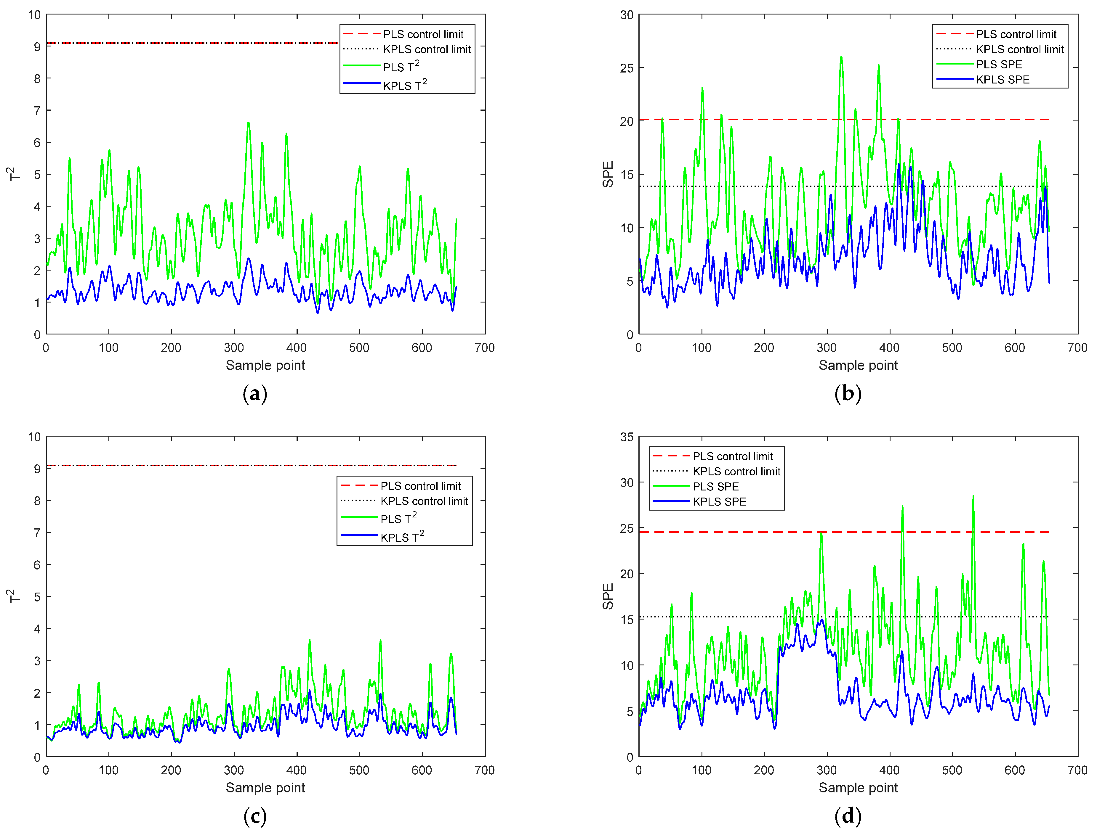
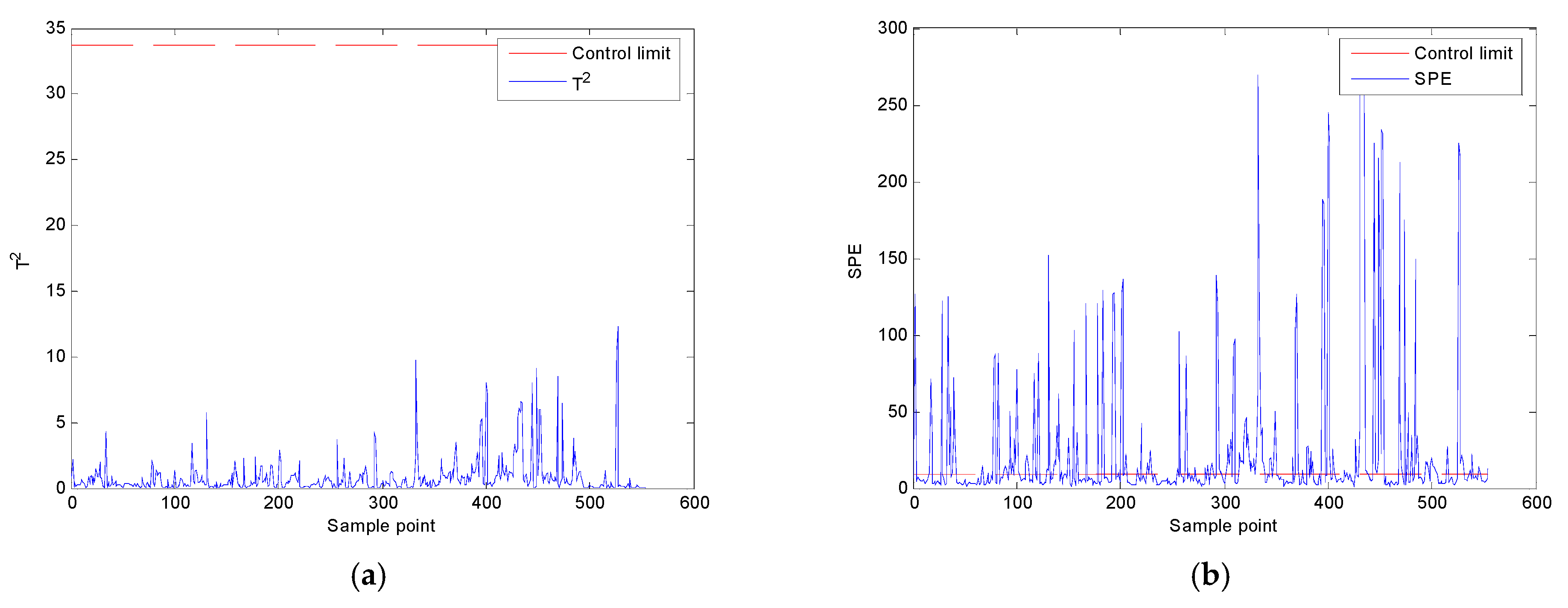
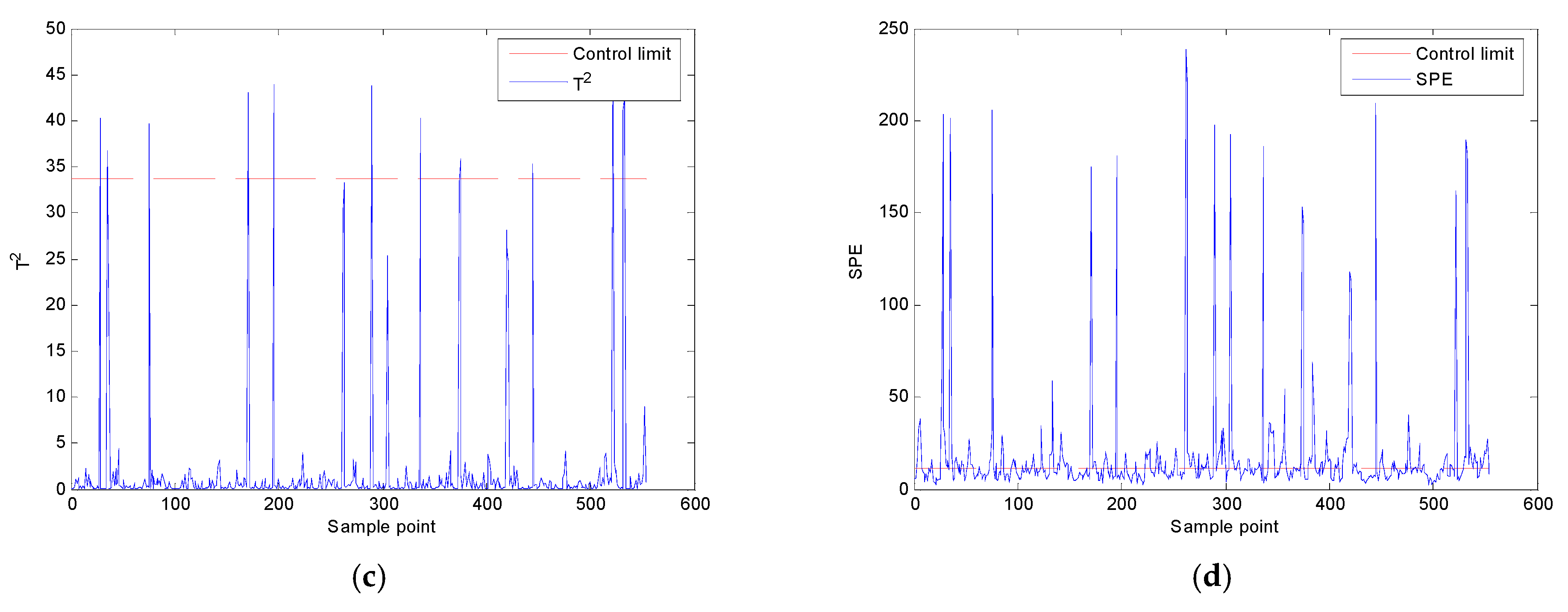
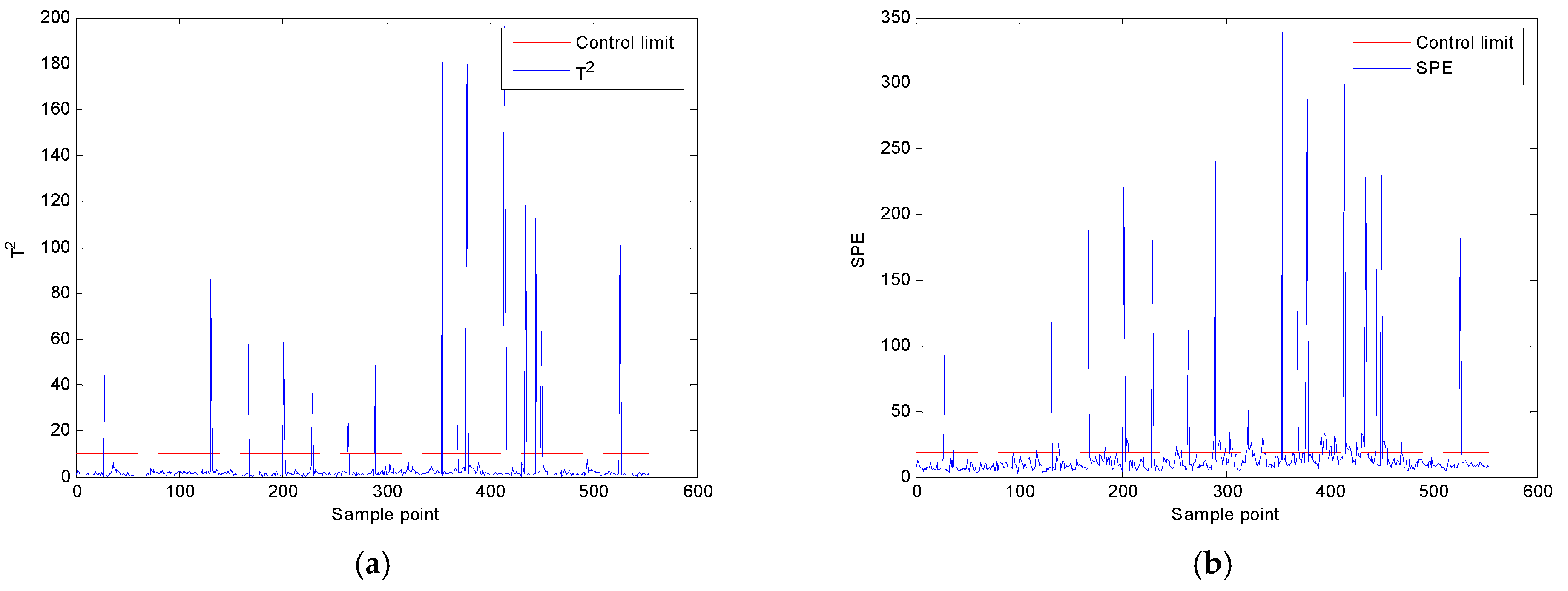
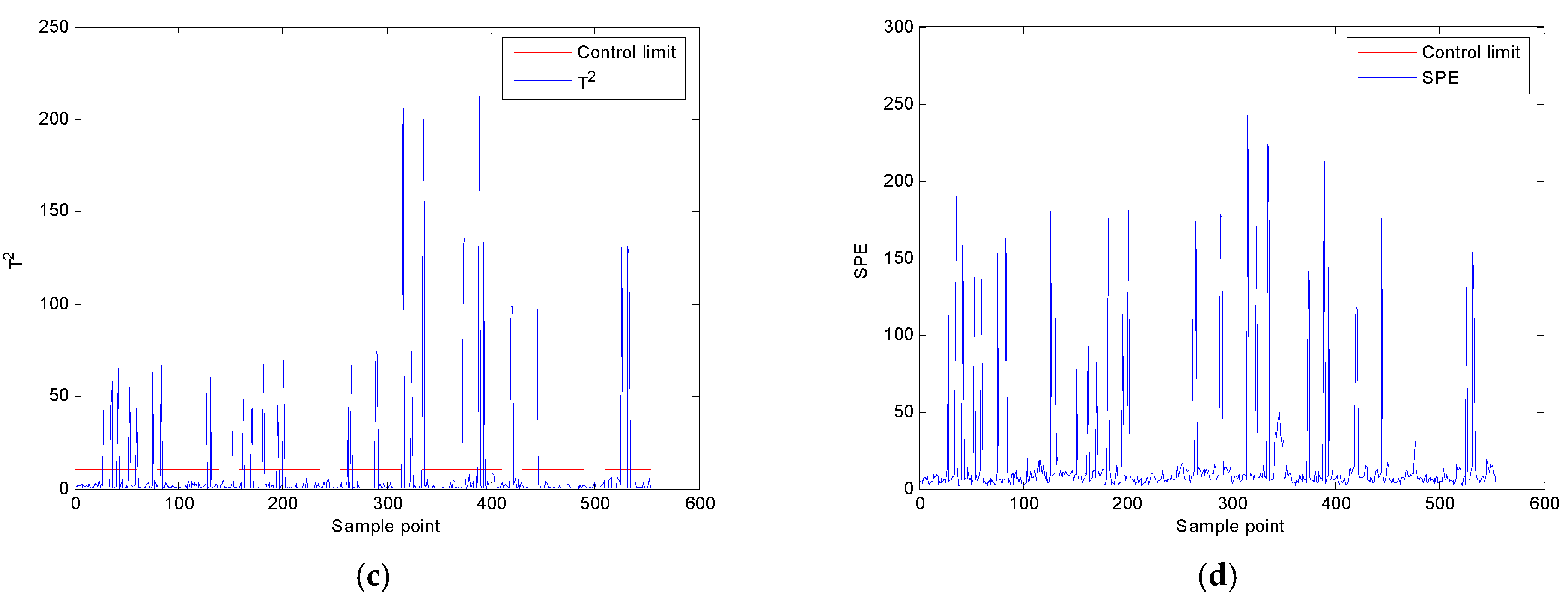
Finally, a faulty process is introduced for monitoring. Firstly, the monitoring results of faulty test data 1 and test data 2 are obtained, and are shown in Figure 10a–d, respectively. For Mode 1, the T2 statistic is beneath the control limit, while the SPE statistic goes beyond the control limit, which means the test data are in a faulty status. For Mode 2, both the T2 statistic and SPE statistic go beyond their control limits, which means the test data are in a faulty status. It can be seen that faulty process monitoring by the single-mode mean matrix KPLS model provides satisfactory monitoring results. Secondly, the monitoring results of faulty test data 1 and test data 2 are monitored by the combined model of the two modes, respectively. The monitoring results are represented in Figure 11a–d. Both the T2 and SPE statistics go beyond their control limits, which means the test data are in a faulty status. In addition, the monitoring results of the multimode mean matrix KPLS model can also provide satisfactory monitoring results. When a fault occurs, it can be monitored and identified correctly.
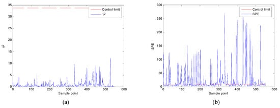
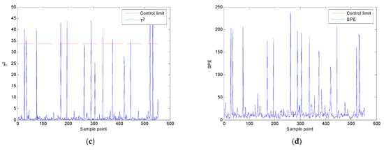
Figure 10.
Mach number monitoring results of a faulty test: (a) T2 for Mode 1; (b) SPE for Mode 1; (c) T2 for Mode 2; (d) SPE for Mode 2.
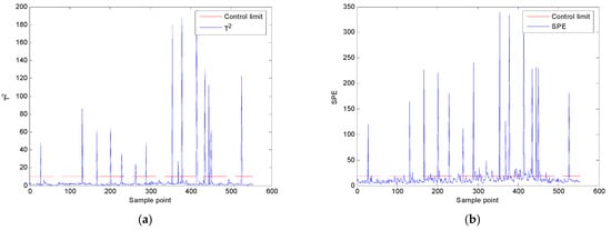

Figure 11.
Multimode Mach number monitoring results of a faulty test: (a) T2 for test data 1; (b) SPE for test data 1; (c) T2 for test data 2; (d) SPE for test data 2.
Based on the previous illustration, the implication derived after the Mach number prediction section, i.e., that the monitoring based on the mean matrix KPLS model would be more reliable than that based on the mean matrix PLS model, has been proven.
In summary, the simulation section shows the application outcomes of the proposed Mach number prediction results, followed by the monitoring results based on the mean matrix KPLS method. Before further analysis, typical working conditions are divided into two modes, and following analysis is focused on Mode 1, Mode 2, and the multiple modes. During the Mach number prediction, the mean matrix KPLS model provides better predictions than the mean matrix PLS model, which proves the efficiency of the kernel function in handling the nonlinear problem. Meanwhile, the single-mode models for Mode 1 and Mode 2 can offer better predictions than the multimode model, which proves the necessity of mode analysis and mode division. Furthermore, based on the more precise prediction of the Mach number, process monitoring for the two modes is conducted. Additionally, the monitoring results of the mean matrix KPLS model are compared with those of the mean matrix PLS model, and both the results of the single-mode model and the results of the multimode model are obtained and observed. Finally, fault process data are monitored by both the single-mode model and the results of the multimode model. Both of these models can offer satisfactory monitoring results. Since the single-mode model is better at predicting the Mach number, it is also preferred in Mach number monitoring.
4. Conclusions
A strategy for Mach number monitoring is introduced in this paper on the basis of the prediction of the Mach number for a multimode wind tunnel system. First, mean matrix KPLS models are established to obtain the Mach number predictions. Secondly, based on the Mach number predictions, a process monitoring strategy is proposed based on T2 and SPE statistics and their control limits. In application, better predictions are achieved based on proper mode division. Through the comparison with PLS, KPLS is superior at solving the nonlinear problem, providing better prediction and satisfactory monitoring results.
Author Contributions
Conceptualization, J.G.; methodology, W.M.; software, R.Z.; validation, X.C.; formal analysis, W.M.; investigation, W.M.; resources, X.C.; data curation, R.Z.; writing—original draft preparation, W.M.; writing—review and editing, L.Z.; visualization, W.M.; supervision, J.G.; project administration, R.Z.; funding acquisition, X.C. All authors have read and agreed to the published version of the manuscript.
Funding
This research was funded by the National Natural Science Foundation of China (No. 61503069) and the Fundamental Research Funds for the Central Universities (N150404020).
Data Availability Statement
Not applicable.
Conflicts of Interest
The authors declare no conflict of interest.
References
- Ju, X.F.; Wang, X.L.; Gao, Y. Wind tunnel flow field model predictive control based on multi-model. Control Eng. China 2018, 25, 1830–1835. [Google Scholar]
- Zhang, T.F.; Mao, Z.Z.; Yuan, P. Modeling of wind tunnel system based on nonlinear block-oriented model. Control Theory Appl. 2016, 33, 413–421. [Google Scholar]
- Yu, F.; Yuan, P.; Mao, Z.Z. Recursive identification of stagnation pressure in wind tunnel system. In Proceedings of the 35th Chinese Control Conference, Chengdu, China, 27–29 July 2016. [Google Scholar]
- Wang, X.J.; Yuan, P.; Mao, Z.Z.; Du, N. Wind tunnel Mach number prediction model based on random forest. Acta Aeronaut. Astronaut. Sin. 2016, 37, 1494–1505. [Google Scholar]
- Du, N.; Jiang, J.Y.; Yu, W.S.; Chen, L. Application of Ensemble Neural Network in the Prediction of Mach Number in 2.4 m Transonic Wind Tunnel. Ordnance Ind. Autom. 2015, 34, 56–58. [Google Scholar]
- Guo, J.; Zhang, R.; Cui, X.C.; Huang, X.; Zhao, L.P. Mach number prediction and analysis of multi-mode wind tunnel system. In Proceedings of the 2020 Chinese Automation Congress (CAC), Shanghai, China, 6–8 November 2020; pp. 6895–6900. [Google Scholar]
- Yuan, P.; Zhao, L.P. KPLS-based Mach number prediction for multi-mode wind tunnel flow system. Processes 2022, 10, 1718. [Google Scholar] [CrossRef]
- Geladi, P.; Kowalshi, B.R. Partial least squares regression: A tutorial. Anal. Chim. Acta 1986, 185, 1–17. [Google Scholar] [CrossRef]
- Kourti, T.; MacGregor, J.F. Process analysis, monitoring and diagnosis, using multivariate projection methods. Chemom. Intell. Lab. Syst. 1995, 28, 3–21. [Google Scholar] [CrossRef]
- Wang, X.Z. Data Mining and Knowledge Discovery for Process Monitoring and Control; Springer: Berlin/Heidelberg, Germany, 1999. [Google Scholar]
- Gurden, S.P.; Westerhuis, J.A.; Bro, R.; Smilde, A.K. A comparison of multiway regression and scaling methods. Chemom. Intell. Lab. Syst. 2001, 59, 121–136. [Google Scholar] [CrossRef]
- Wang, H.W. Partial Least Squares Regression Method and Its Application; National Defense Industry Press: Beijing, China, 1999. [Google Scholar]
- Nomikos, P.; MacGregor, J.F. Multi-way partial least squares in monitoring batch processes. Chemom. Intell. Lab. Syst. 1995, 30, 97–108. [Google Scholar] [CrossRef]
- Wangen, L.E.; Kowalski, B.R. A multiblock partial least squares algorithm for investigating complex chemical systems. J. Chemom. 1988, 3, 3–20. [Google Scholar] [CrossRef]
- MacGregor, J.F.; Jackle, C.; Kiparissides, C. Process monitoring and diagnosis by multiblock PLS methods. AIChE J. 1994, 40, 826–838. [Google Scholar] [CrossRef]
- Rosipal, R.; Trejo, L.J. Kernel partial least squares regression in reproducing kernel Hilbert space. J. Mach. Learn. Res. 2001, 2, 97–123. [Google Scholar]
- Zhang, X.; Kano, M.; Li, Y. Locally weighted kernel partial least squares regression based on sparse nonlinear features for virtual sensing of nonlinear time-varying processes. Comput. Chem. Eng. 2017, 104, 164–171. [Google Scholar] [CrossRef]
- Lee, J.M.; Yoo, C.K.; Sang, W.C.; Vanrolleghem, P.A.; Lee, I.B. Nonlinear process monitoring using kernel principal component analysis. Chem. Eng. Sci. 2004, 59, 223–234. [Google Scholar] [CrossRef]
- Zhou, P.; Liu, J.P.; Liang, M.Y.; Zhang, R.Y. KPLS robust reconstruction error based monitoring and anomaly dentification of fuel ratio in blast furnace ironmaking. Acta Autom. Sin. 2021, 47, 1661–1671. [Google Scholar]
- Jia, R.D.; Mao, Z.Z.; Wang, F.L. KPLS model based product quality control for batch processes. CIESC J. 2013, 64, 1332–1339. [Google Scholar]
- Lu, N.Y.; Gao, F.R. Stage-based process analysis and quality prediction for batch processes. Ind. Eng. Chem. Res. 2005, 44, 3547–3555. [Google Scholar] [CrossRef]
- Jategaonkar, R. Flight Vehicle System Identification: A Time Domain Methodology; AIAA: Reston VA, USA, 2015. [Google Scholar]


Disclaimer/Publisher’s Note: The statements, opinions and data contained in all publications are solely those of the individual author(s) and contributor(s) and not of MDPI and/or the editor(s). MDPI and/or the editor(s) disclaim responsibility for any injury to people or property resulting from any ideas, methods, instructions or products referred to in the content. |
© 2023 by the authors. Licensee MDPI, Basel, Switzerland. This article is an open access article distributed under the terms and conditions of the Creative Commons Attribution (CC BY) license (https://creativecommons.org/licenses/by/4.0/).