


A Moving Window Double Locally Weighted Extreme Learning Machine on an Improved Sparrow Searching Algorithm and Its Case Study on a Hematite Grinding Process


Abstract
1. Introduction
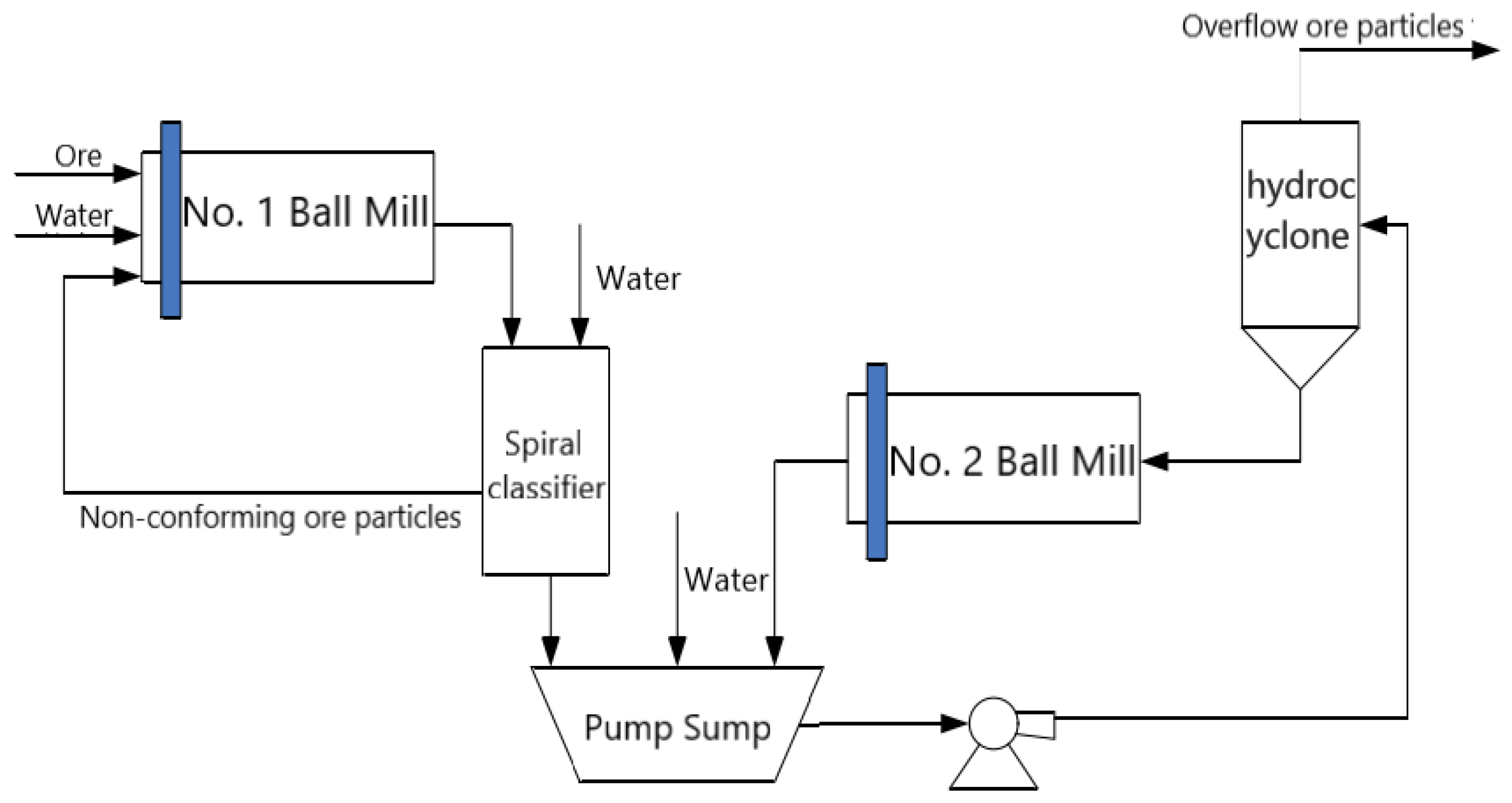
2. The Grinding Particle Size in Hematite Grinding Process
3. A Double Locally Weighted Extreme Learning Machine Based on Moving Window for the Grinding Particle Size Modeling
3.1. The Basic Principle of the Extreme Learning Machine
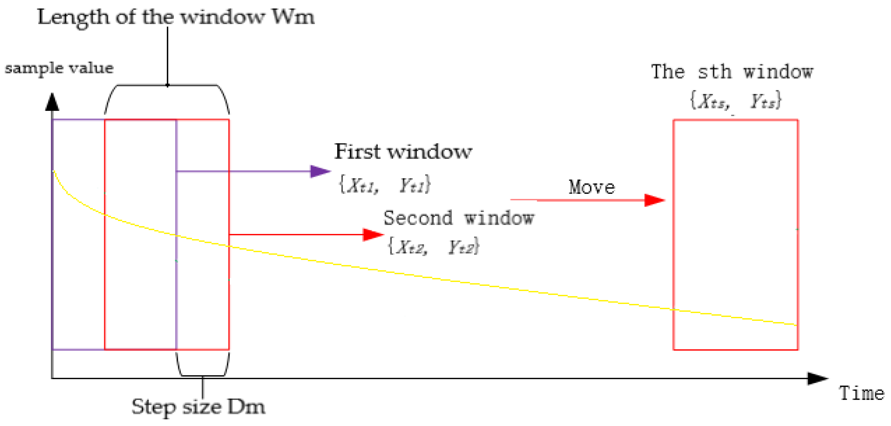
3.2. A Double Locally Weighted Extreme Learning Machine Based on Moving Window Technology
4. Parameter Optimization Based on Improved Sparrow Optimization Algorithm
4.1. Parameter Optimization for the MW-DLW-ELM Model
4.2. Original Sparrow Searching Algorithm
4.3. Improved Sparrow Searching Algorithm
- Producers:
- Followers:
| Algorithm 1: Improved Sparrow Searching Algorithm |
| Input: Generate random population of sparrows Xi(t) |
| Output: Xi(t + 1) and F(Xi(t + 1))(Fitness value) |
| 1: Initialize population parameters, such as population number, the maximum number of iterations Itermax, discoverers PD, number of early warning sparrows SD, warning threshold R2, etc. |
| 2: Calculate the fitness value of each sparrow, find the current optimal individual fitness values, the worst fitness and the corresponding location. |
| 3: The producers were selected from the sparrows with better position, and the producer updates the position by Equation (23). |
| 4: The remaining sparrows act as followers and update the position by Equation (24). |
| 5: Select some sparrows randomly among the sparrows as scout and update the position by Equation (26). |
| 6: Calculate the updated fitness of the entire sparrow population and find the global optimal sparrow. |
| 7: Determine if the end condition is met, and if so, proceed to the next step, otherwise jump to step 2. |
| 8: The program ends and the optimal result is output. |
5. Experiments and Analysis
5.1. Experiment of Benchmark Function
5.2. Experiments on the Parameters Optimization of the ELM Models
6. Conclusions
Author Contributions
Funding
Data Availability Statement
Conflicts of Interest
References
- Sbarbaro, D.; Del Villar, R. Advanced Control and Supervision of Mineral Processing Plants; Springer: London, UK, 2010. [Google Scholar]
- Wang, M.H.; Yang, R.Y.; Yu, A.B. DEM investigation of energy distribution and particle breakage in tumbling ball mills. Powder Technol. 2012, 223, 83–91. [Google Scholar] [CrossRef]
- Chai, T.Y.; Ding, J.L. Hybrid intelligent control for optimal operation of shaft furnace roasting process. Control. Eng. Pract. 2011, 19, 264–275. [Google Scholar] [CrossRef]
- Lu, S.; Zhou, P.; Chai, T.Y.; Dai, W. Modeling and simulation of whole ball mill grinding plant for integrated control. IEEE Trans. Autom. Sci. Eng. 2014, 11, 1004–1019. [Google Scholar]
- Zhou, P.; Chai, T.Y.; Wang, H. Intelligent optimal-setting control for grinding circuits of mineral processing process. IEEE Trans. Autom. Sci. Eng. 2009, 6, 730–743. [Google Scholar] [CrossRef]
- Wei, D.H.; Craig, I.K. Grinding mill circuits-a survey of control and economic concerns. Int. J. Miner. Process. 2009, 90, 56–66. [Google Scholar] [CrossRef]
- Zhou, P.; Lu, S.; Yuan, M.; Chai, T.Y. Survey on higher-level advanced control for grinding circuits operation. Powder Technol. 2016, 288, 324–338. [Google Scholar] [CrossRef]
- Brics, M.; Ints, V.; Kitenbergs, G.; Cebers, A. The most energetically favorable configurations of hematite cube chains. Phys. Rev. E 2021, 105, 024605. [Google Scholar] [CrossRef]
- Zhou, P.; Chai, T.Y.; Sun, J. Intelligence-Based Supervisory Control for Optimal Operation of a DCS-Controlled Grinding System. IEEE Trans. Control Syst. Technol. 2013, 21, 143–148. [Google Scholar] [CrossRef]
- Mitchell, T.M. Machine Learning; McGrawHill: New York, NY, USA, 1997. [Google Scholar]
- Guan, S.H.; Shen, Y.X. Power load forecasting based on PSO RBF-NN. Transducer Microsyst. Technol. 2021, 40, 128–131. [Google Scholar]
- Cortes, C.; Vapnik, V. Support-vector networks, Mach. Learn. 1995, 20, 273–297. [Google Scholar]
- Sannasi Chakravarthy, S.; Bharanidharan, N.; Rajaguru, H. Multi-deep CNN based experimentations for early diagnosis of breast cancer. IETE J. Res. 2022, 1–16. [Google Scholar] [CrossRef]
- Huang, G.B.; Zhu, Q.Y.; Siew, C. Extreme learning machine: Theory and applications. Neurocomputing. 2006, 70, 489–501. [Google Scholar] [CrossRef]
- Du, Y.G.; Del Villar, R.; Thibault, J. Neural net-based softsensor for dynamic particle size estimation in grinding circuits. Int. J. Miner. Process. 1997, 52, 121–135. [Google Scholar] [CrossRef]
- Del Villar, R.G.; Thibault, J.; Del Villar, R. Development of a softsensor for particle size monitoring. Miner. Eng. 1996, 9, 55–72. [Google Scholar] [CrossRef]
- Sun, Z.; Wang, H.; Zhang, Z. Soft sensing of overflow particle size distributions in hydrocyclones using a combined method. Tsinghua Sci. Technol. 2008, 13, 47–53. [Google Scholar] [CrossRef]
- Ding, J.L.; Chai, T.Y.; Cheng, W.J.; Zheng, X.P. Data-based multiple-model prediction of the production rate for hematite ore beneficiation process. Control Eng. Practice. 2015, 45, 219–229. [Google Scholar] [CrossRef]
- Deris, A.M.; Zain, A.M.; Sallehuddin, R. Overview of support vector machine in modeling machining performances. In Proceedings of the 2011 International Conference on Advances in Engineering, Shanghai, China, 17–18 September 2011. [Google Scholar]
- Tang, J.; Chai, T.Y.; Zhao, L.J.; Yu, W.; Yue, H. Soft sensor for parameters of mill load based on multi-spectral segments PLS sub-models and on-line adaptive weighted fusion algorithm. Neurocomputing 2012, 78, 38–47. [Google Scholar] [CrossRef]
- Meng, A.B.; Zhu, Z.B.; Deng, W.S.; Ou, Z.H.; Lin, S.; Wang, C.; Xu, X.; Wang, X.L.; Yin, H.; Luo, J.Q. A novel wind power prediction approach using multivariate variational mode decomposition and multi-objective crisscross optimization based deep extreme learning machine. Energy 2022, 260, 124957–124977. [Google Scholar] [CrossRef]
- Deepika, K.K.; Varma, P.S.; Reddy, C.R.; Sekhar, O.C.; Alsharef, M.; Alharbi, Y.; Alamri, B. Comparison of Principal-Component-Analysis-Based Extreme Learning Machine Models for Boiler Output Forecasting. Appl. Sci. 2022, 12, 7671–7686. [Google Scholar] [CrossRef]
- Yuan, X.F.; Ge, Z.Q.; Huang, B.; Song, Z.H. A probabilistic just-in-time learning framework for soft sensor development with missing data. IEEE Trans. Control Syst. Technol. 2016, 25, 1124–1132. [Google Scholar] [CrossRef]
- Yang, Z.; Ge, Z.Q. Rethinking the value of just-in-time learning in the era of industrial big data. IEEE Trans. Ind. Inform. 2021, 18, 976–985. [Google Scholar] [CrossRef]
- Hu, Y.; Ma, H.H.; Shi, H.B. Enhanced batch process monitoring using just-in-time-learning based kernel partial least squares. Chemometrics Intell. Lab. Syst. 2013, 123, 15–27. [Google Scholar] [CrossRef]
- Bai, Y.; Zhang, G.Q.; Wang, G.L.; Chen, F.F.; Bi, G.D.; Xu, D.G. Position and speed detection method based on adaptive extended moving-window linear regression for traction machine drives. IEEE Trans. Transport. Electrific. 2022, 8, 2884–2897. [Google Scholar] [CrossRef]
- Yuan, X.F.; Ge, Z.Q.; Song, Z.H. Spatio-temporal adaptive soft sensor for nonlinear time-varying and variable drifting processes based on moving window LWPLS and time difference model. Asia-Pac. J. Chem. Eng. 2016, 11, 209–219. [Google Scholar] [CrossRef]
- Chen, J.Y.; Gui, W.H.; Dai, J.Y.; Yuan, X.F.; Chen, N. An ensemble just-in-time learning soft-sensor model for residual lithium concentration prediction of ternary cathode materials. J. Chemometr. 2020, 34, 3225–3240. [Google Scholar] [CrossRef]
- Dai, J.Y.; Chen, N.; Luo, B.; Gui, W.H.; Yang, C.H. Multi-scale local LSSVM based spatiotemporal modeling and optimal control for the goethite process. Neurocomputing 2020, 385, 88–99. [Google Scholar] [CrossRef]
- Dai, J.Y.; Chen, N.; Yuan, X.F.; Gui, W.H.; Luo, L.H. Temperature prediction for roller kiln based on hybrid first-principle model and data-driven MW-DLWKPCR model. ISA Trans. 2020, 98, 403–417. [Google Scholar] [CrossRef]
- Yuan, X.F.; Zhou, J.; Wang, Y.L.; Yang, C.H. Multi-similarity measurement driven ensemble just-in-time learning for soft sensing of industrial processes. J. Chemometr. 2018, 32, 3040–3053. [Google Scholar] [CrossRef]
- Pan, B.; Jin, H.P.; Wang, L.; Qian, B.; Chen, X.G.; Huang, S.; Li, J.G. Just-in-time learning based soft sensor with variable selection and weighting optimized by evolutionary optimization for quality prediction of nonlinear processes. Chem. Eng. Res. Des. 2019, 144, 285–299. [Google Scholar] [CrossRef]
- Ding, Y.Y.; Wang, Y.Q.; Zhou, D.H. Mortality prediction for ICU patients combining just-in-time learning and extreme learning machine. Neurocomputing 2018, 281, 12–19. [Google Scholar] [CrossRef]
- Peng, X.; Tang, Y.; Du, W.L.; Qian, F. Online performance monitoring and modeling paradigm based on just-in-time learning and extreme learning machine for a non-Gaussian chemical process. Ind. Eng. Chem. Res. 2017, 56, 6671–6684. [Google Scholar] [CrossRef]
- Xue, J.K.; Shen, B. A novel swarm intelligence optimization approach: Sparrow search algorithm. Syst. Sci. Control Eng. 2020, 8, 22–34. [Google Scholar] [CrossRef]
- Oliva, D.; Aziz, M.A.E.; Hassanien, A.E. Parameter estimation of photovoltaic cells using an improved chaotic whale optimization algorithm. Appl. Energy 2017, 200, 141–154. [Google Scholar] [CrossRef]
- Hezagy, A.E.; Makhlouf, M.A.; El-tawel, S.G. Improved salp swarm algorithm for feature selection. J. King Saud Univ.-Comput. Inf. Sci. 2020, 32, 335–344. [Google Scholar]
- Wang, X.W.; Wang, W.; Wang, Y. An adaptive bat algorithm. In Proceedings of the 9th International Conference on Intelligent Computing Theories and Technology, Nanning, China, 28–31 July 2013. [Google Scholar]
- Li, J.; Luo, Y.K.; Wang, C.; Zeng, Z.G. Simplified particle swarm algorithm based on nonlinear decrease extreme disturbance and Cauchy mutation. Int. J. Parallel Emerg. Distrib. Syst. 2020, 35, 236–245. [Google Scholar] [CrossRef]
- Wang, W.H.; Xu, L.; Chau, K.W.; Xu, D.M. Yin-Yang firefly algorithm based on dimensionally Cauchy mutation. Expert Syst. Appl. 2020, 150, 113216–113232. [Google Scholar] [CrossRef]
- Xu, Y.T.; Chen, H.L.; Luo, J.; Zhang, Q.; Jiao, S.; Zhang, X.Q. Enhanced Moth- flame optimizer with mutation strategy for global optimization. Inf. Sci. 2019, 492, 181–203. [Google Scholar] [CrossRef]
- Pappula, L.; Ghosh, D. Synthesis of linear aperiodic array using Cauchy mutated cat swarm optimization. AEU-Int. J. Electron. Commun. 2017, 72, 52–64. [Google Scholar] [CrossRef]
- Farah, A.; Belazi, A.; Alqunun, K.; Almalaq, A.; Alshammari, B.M.; Ben Hamida, M.B.; Abbassi, R. A New Design Method for optimal parameters setting of PSSs and SVC damping controllers to alleviate power system stability problem. Energies 2021, 14, 7312–7337. [Google Scholar] [CrossRef]
- Dong, J.; Dou, Z.H.; Si, S.Q.; Wang, Z.C.; Liu, L.X. Optimization of capacity configuration of wind–solar–diesel–storage using improved sparrow search algorithm. J. Electr. Eng. Technol. 2022, 17, 1–14. [Google Scholar] [CrossRef]
- Ding, C.; Ding, Q.C.; Wang, Z.Y.; Zhou, Y.Y. Fault diagnosis of oil-immersed transformers based on the improved sparrow search algorithm optimised support vector machine. IET Electr. Power Appl. 2022, 16, 985–995. [Google Scholar] [CrossRef]
- Kennedy, J.; Eberhart, R. Particle Swarm Optimization. In Proceedings of the IEEE International Conference on Neural Networks, Perth, Australia, 27 November–1 December 1995. [Google Scholar]
- Mirjalili, S.; Mirjalili, S.M.; Lewis, A. Grey wolf optimizer. Adv. Eng. Softw. 2014, 69, 46–61. [Google Scholar] [CrossRef]


| Test Function Expression | Symbol | Range of Values | Value of Optimal Solution |
|---|---|---|---|
| F1 | [−100, 100] | 0 | |
| F2 | [−10, 10] | 0 | |
| F3 | [−100, 100] | 0 | |
| F4 | [−100, 100] | 0 | |
| F5 | [−1.28, 1.28] | 0 | |
| F6 | [−5.12, 5.12] | 0 | |
| F7 | [−30, 30] | 0 | |
| F8 | [−600, 600] | 0 | |
| F9 | [−65.536, 65.536] | 1 | |
| F10 | [0, 10] | 1/ci | |
| F11 | [0, 1] | −3.8628 |
| Functions | PSO | GWO | SSA | ISSA | Optimal Value | |
|---|---|---|---|---|---|---|
| F1 | Best | 0.058933 | 3.396 × 10−62 | 1.714 × 10−158 | 0 | 0 |
| Worst | 0.38873 | 7.5113 × 10−58 | 2.3176 × 10−75 | 0 | ||
| Mean | 0.19735 | 6.8668 × 10−59 | 7.7423 × 10−77 | 0 | ||
| STD | 0.092988 | 1.5269 × 10−58 | 4.231 × 10−76 | 0 | ||
| F2 | Best | 1.3475 | 4.0876 × 10−36 | 2.9828 × 10−84 | 7.0841 × 10−250 | 0 |
| Wort | 7.7625 | 3.8835 × 10⁻³⁴ | 8.8405 × 10−41 | 2.6869 × 10−223 | ||
| Mean | 3.4671 | 8.7556 × 10⁻³⁵ | 3.2694 × 10−42 | 8.9563 × 10−225 | ||
| STD | 1.5434 | 8.292 × 10⁻³⁵ | 1.6118 × 10−41 | 0 | ||
| F3 | Best | 6.6321 | 3.061 × 10⁻¹⁹ | 0 | 0 | 0 |
| Worst | 32.7164 | 2.8866 × 10⁻¹³ | 7.7326 × 10⁻³⁵ | 0 | ||
| Mean | 17.1663 | 1.1034 × 10⁻¹⁴ | 2.7878 × 10−36 | 0 | ||
| STD | 7.6494 | 5.2766 × 10⁻¹⁴ | 1.4122 × 10⁻³⁵ | 0 | ||
| F4 | Best | 1.0528 | 5.2743 × 10⁻¹⁶ | 9.227 × 10−166 | 6.6986 × 10−243 | 0 |
| Worst | 4.7375 | 2.3154 × 10⁻¹⁴ | 1.2678 × 10⁻³¹ | 1.6359 × 10−222 | ||
| Mean | 2.8452 | 8.8794 × 10⁻¹⁵ | 4.245 × 10⁻³³ | 5.7244 × 10−224 | ||
| STD | 1.1379 | 5.607 × 10⁻¹⁵ | 2.3144 × 10⁻³² | 0 | ||
| F5 | Best | 0.043813 | 0.00019499 | 0.0001679 | 1.9965 × 10⁻⁵ | 0 |
| Worst | 5.3953 | 0.0020989 | 0.0013119 | 0.00040725 | ||
| Mean | 0.28151 | 0.0007823 | 0.0033844 | 0.0016521 | ||
| STD | 0.96657 | 0.00048393 | 0.0010085 | 0.00034993 |
| Functions | PSO | GWO | SSA | ISSA | Optimal Value | |
|---|---|---|---|---|---|---|
| F6 | Best | 24.2468 | 0 | 0 | 0 | 0 |
| Worst | 84.1836 | 4.8221 | 0 | 0 | ||
| Mean | 53.8561 | 14.4021 | 0 | 0 | ||
| STD | 14.4021 | 1.1637 | 0 | 0 | ||
| F7 | Best | 2.5838 | 1.1546 × 10⁻¹⁴ | 8.8818 × 10⁻¹⁶ | 8.8818 × 10⁻¹⁶ | 0 |
| Worst | 6.5662 | 2.2204 × 10⁻¹⁴ | 8.8818 × 10⁻¹⁶ | 8.8818 × 10⁻¹⁶ | ||
| Mean | 4.1938 | 1.5336 × 10⁻¹⁴ | 8.8818 × 10⁻¹⁶ | 8.8818 × 10⁻¹⁶ | ||
| STD | 0.93679 | 1.8504 × 10⁻¹⁵ | 0 | 0 | ||
| F8 | Best | 2.4427 | 0 | 0 | 0 | 0 |
| Worst | 14.703 | 0.021561 | 0 | 0 | ||
| Mean | 5.8382 | 0.0021043 | 0 | 0 | ||
| STD | 2.7263 | 0.0055966 | 0 | 0 | ||
| F9 | Best | 0.998 | 0.998 | 0.998 | 0.998 | 1 |
| Worst | 5.9288 | 10.7632 | 12.6705 | 0.998 | ||
| Mean | 1.5932 | 3.6837 | 4.6346 | 0.998 | ||
| STD | 1.0887 | 3.3394 | 5.2536 | 1.3039 × 10⁻¹⁶ | ||
| F10 | Best | −10.1532 | −10.1531 | −10.1532 | −10.1532 | −10.1532 |
| Worst | −2.6305 | −4.145 | −5.0552 | −10.1532 | ||
| Mean | −6.1408 | −9.4457 | −8.7937 | −10.1532 | ||
| STD | 3.2554 | 1.8396 | 2.2929 | 5.8915 × 10⁻¹⁵ | ||
| F11 | Best | −3.8628 | −3.8628 | −3.8628 | −3.8628 | −3.8628 |
| Worst | −3.8549 | −3.8549 | −3.0898 | −3.8628 | ||
| Mean | −3.8617 | −3.8612 | −3.837 | −3.8628 | ||
| STD | 0.002725 | 0.0028854 | 0.14113 | 2.6402 × 10⁻¹⁵ |
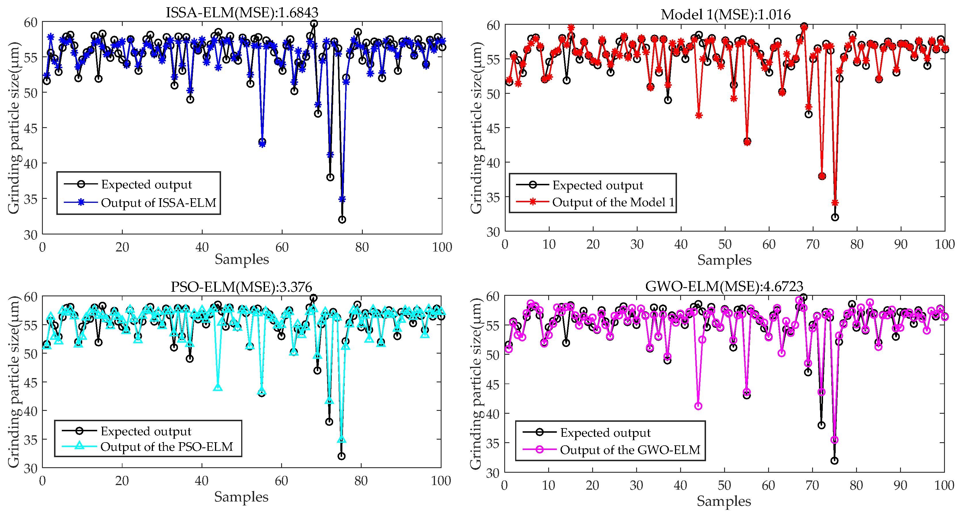
| Model | MAX | MSE | MAE |
|---|---|---|---|
| ISSA-ELM | 4.1087 | 1.6843 | 0.9377 |
| Model 1 | 2.1324 | 1.0160 | 0.4926 |
| PSO-ELM | 5.8202 | 3.3760 | 0.9165 |
| GWO-ELM | 6.4012 | 4.6723 | 0.9704 |
Disclaimer/Publisher’s Note: The statements, opinions and data contained in all publications are solely those of the individual author(s) and contributor(s) and not of MDPI and/or the editor(s). MDPI and/or the editor(s) disclaim responsibility for any injury to people or property resulting from any ideas, methods, instructions or products referred to in the content. |
© 2023 by the authors. Licensee MDPI, Basel, Switzerland. This article is an open access article distributed under the terms and conditions of the Creative Commons Attribution (CC BY) license (https://creativecommons.org/licenses/by/4.0/).
Share and Cite
Liu, H.; Dai, J.; Chen, X. A Moving Window Double Locally Weighted Extreme Learning Machine on an Improved Sparrow Searching Algorithm and Its Case Study on a Hematite Grinding Process. Processes 2023, 11, 169. https://doi.org/10.3390/pr11010169
Liu H, Dai J, Chen X. A Moving Window Double Locally Weighted Extreme Learning Machine on an Improved Sparrow Searching Algorithm and Its Case Study on a Hematite Grinding Process. Processes. 2023; 11(1):169. https://doi.org/10.3390/pr11010169
Chicago/Turabian StyleLiu, Huating, Jiayang Dai, and Xingyu Chen. 2023. "A Moving Window Double Locally Weighted Extreme Learning Machine on an Improved Sparrow Searching Algorithm and Its Case Study on a Hematite Grinding Process" Processes 11, no. 1: 169. https://doi.org/10.3390/pr11010169
APA StyleLiu, H., Dai, J., & Chen, X. (2023). A Moving Window Double Locally Weighted Extreme Learning Machine on an Improved Sparrow Searching Algorithm and Its Case Study on a Hematite Grinding Process. Processes, 11(1), 169. https://doi.org/10.3390/pr11010169