Comparison of Experimental Results from Operating a Novel Fluidized Bed Classifier with CFD Simulations Applying Different Drag Models and Model Validation ^†

Abstract

A cold-flow lab-scale cross-flow fluidized bed classifier was simulated using the CFD software Barracuda VR^®. The purpose of the study was to identify the most suitable drag model and make the model adjustments that provide the best representation of the flow situation in the classifier when comparing the results with the experimental data. Two particle types were used in the simulations and in the experiments: zirconia (median diameter 69 µm, skeletal density 3830 kg/m³) and steel (290 µm, 7790 kg/m³). Ten different cases, with different solids loading values, were investigated: three with pure zirconia particles, three with pure steel particles, and four with a mixture of zirconia (28%) and steel (72%). Several different drag models were tried out in the simulations. However, none of the available models were able to predict the classification efficiency observed in experiments with their default settings. Although most of the drag models correctly predicted the inversely proportional behavior of the classification efficiency vs. solids loading, the classification efficiency was overpredicted. It was observed that a combined WenYu/Ergun drag model gave a wide range of accuracy, by being able to capture the behavior of both dense and dilute particle systems. Even though the predictions of the classification efficiency for steel particles were acceptable, a larger deviation was observed with Geldart A zirconia particles. CFD simulations with the WenYu and Ergun combined drag model were used for further validation against the experimental observations. In this case, previously published experimental data for fluidization of pure Zirconia particles were used. The fluidization of zirconia was modelled in Barracuda VR^® with adjustment of the combined WenYu/Ergun drag model parameter (k₁), to obtain a suitable validation. Furthermore, the effect of adding the blended acceleration model (BAM) for the fluidization simulations is discussed. It was observed that the fixed bed pressure drop was very accurate compared to the experimental observation, but the pressure drop after the fluidization was slightly overpredicted.

1. Introduction

Solid classification is a major area in powder handling, and it is also an important part of many industrial powder processing applications. Previously published work by the authors [1,2] presented a novel particle classification system, based on a cross-flow fluidized bed concept, designed for applications in post-combustion carbon capture plants and operating with indirectly heated calcium looping technology [3]. The purpose of the classifier is to separate a mixture of calcium sorbent particles and inert heat transfer particles. The temperature in the full-scale process is around 910 °C, but for initial testing of the classification concept, experiments were performed in a system down-scaled to cold-flow lab-scale conditions. The focus here is on CFD simulations of the cold-flow lab-scale process, comparing different drag models and to find the most suitable drag model to use in Barracuda VR^® (CPFD Software, Houston, TX, USA). This drag model was then used for further validation of the complete CFD model.

CFD simulations can be used to study the performance of an equipment unit and to try out different alternatives before building the actual unit. When studying classifiers, CFD simulations can provide information about the hydrodynamics of the internal gas–solids behavior, and thereby improve the understanding of flow phenomena observed in experiments.

Technically, it is simpler to build a CFD model for cold-flow conditions in the case of validation, since cold flow experimental results are easier to produce. If it is possible to build a successful CFD model for cold-flow conditions, then the same model could be used to predict the flow conditions at hot-flow/large-scale conditions, provided that the system is properly scaled.

Reyes-Urrutia et al. [4] also studied the OpenFOAM^® and MFiX^® CFD platforms and compared a bubbling fluidized bed. This work studies the performance of two CFD codes, to address a bubbling fluidized bed system at different temperature and heat transfer conditions. They found that MFiX^® gives slightly more accurate results compared to OpenFOAM but with a low versatility for meshing curved geometries, which may lead to a higher computational cost for the same level of accuracy. A similar study was done by Venier et al. [5]. They assessed the performance of ANSYS Fluent^® and OpenFOAM^® on bubbling fluidized bed characteristics with Geldart A, B, and D particles. They observed good predictions from both Ansys Fluent^® and OpenFOAM^® for Geldart B and D particles. However, they slightly favored the use of OpenFOAM^® for Geldart A particles. Soria et al. [6] performed a CFD study on cadmium vaporization during fluidized bed incineration of municipal solid waste. Their study was based on Ansys Fluent^® predicted values from a particulate non-isothermal model. Predictions were then compared with the experiments and a higher accuracy was observed. However, all these simulation studies used a high-resolution mesh, which could be computationally expensive. Multiphase-particle-in-cell (MP-PIC) [7,8] concept was developed as a solution to this longer computation time. The MP-PIC approach, also known as computational particle fluid dynamics (CPFD) [8], adopts the concept of parcels in Eulerian–Lagrangian modeling. Here, a group of particles can be represented by a single parcel, and are just virtual points in the computational domain, not real particles.

The novel cross-flow fluidized bed solid classifier studied in the current work was simulated using the MP-PIC approach. The commercially developed platform known as Barracuda Virtual Reactor^® (Barracuda VR^®) can be applied to large systems. Eulerian description is used to model the gas phase. The velocity, temperature, and density fields are solved using the appropriate conservation and constitutive laws. The discrete Lagrangian approach is used to model the particle phase. As explained by Snider et al. [8,9], there is a strong coupling between the fluid and the particle phases. The particle momentum equation uses the MP-PIC concept, including a relaxation-to-the-mean term to represent damping of the particle velocity fluctuations, due to particle collisions [8,9]. Utilizing the computational particle concept, simulation of large industrial fluidized-bed reactors is possible.

There are several CPFD studies on gas–solid multiphase flow applications, including several types of fluidized beds, with or without chemical reactions. Gas–solid CFD simulations using the MP-PIC method related to bubbling fluidized beds [10,11,12,13,14,15,16,17,18,19], fluidized bed gasifiers [9,20,21,22,23], circulating fluidized beds [24,25,26,27,28,29,30,31,32], turbulent fluidized beds [33], fast fluidization and pneumatic conveying [20,34], powder discharging hoppers [35], and cyclones [36,37,38] are available in the literature.

Nevertheless, there are not many publications available on the simulation of particle classification based on the MP-PIC approach and suitable drag model investigations. Particle segregation, due to the density or size differences, was studied by Vivacqua et al. [11] and Chladek et al. [2].

As part of the current design work, the authors studied [1,2] particle segregation based on size and density differences, which is the basis for the novel fluidized bed classifier discussed in this study.

Chladek et al. [2] studied segregation in a mixture of zirconia and steel particles; the same particle mixture that is used in the present study. Those particles were applied based on down-scaling from hot-flow pilot-scale conditions. Their lab-scale cold-flow experiments and Barracuda simulations [2] indicated that it is possible to achieve a clear separation of such a particle mixture in a fluidized bed. The Ergun and WenYu drag models used in the study gave good predictions of the minimum fluidization velocity for the steel particles, and also for the bed pressure drop. However, the predictions were not very good for the zirconia particles.

In this study, the cold-flow lab-scale classifier discussed by the authors in [1] is simulated using Barracuda VR^® 17.1, to identify which drag model could provide the best representation of the actual flow behavior in the classifier, when using the mixture of steel and zirconia particles mentioned above. The seven different drag models available in Barracuda were tested, and the results were compared with experimental observations.

Later, one of the drag models was fine-tuned to obtain a suitable validation status based on the fluidization experiments performed on a cylindrical fluidized bed rig.

2. Cold-Flow Experimental Setup

There were two types of fluidization experiments performed for the current study, but most of the discussion is focused on the experiments carried out on the novel fluidized bed classifier. Nevertheless, the experiments performed on a cylindrical fluidized bed, and explained below, were applied for the final model validation.

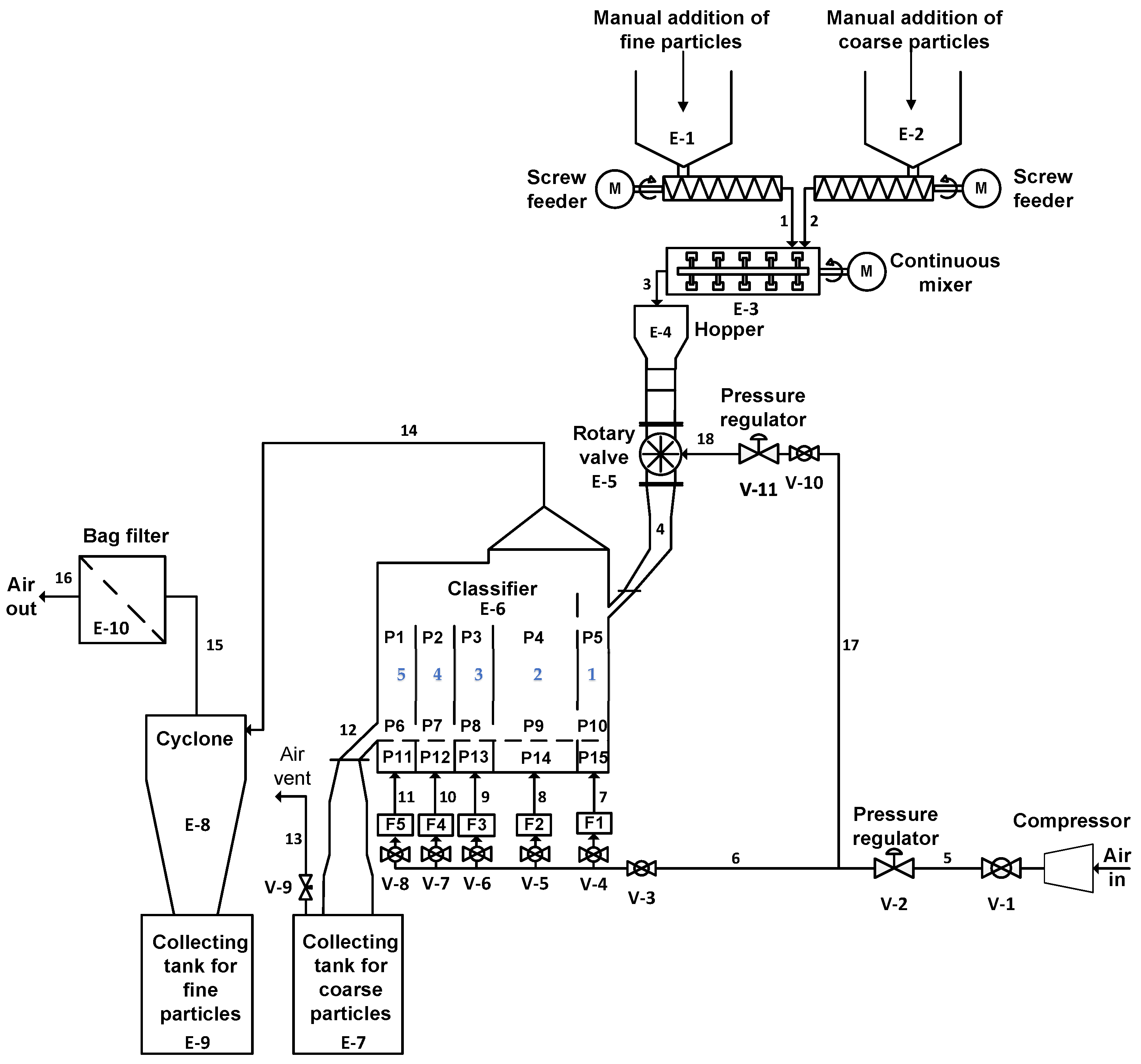
2.1. Fluidized Bed Classifier

Figure 1 shows the cold-flow lab-scale classification rig used in this study. The classifier has one inlet for the particle mixture; five air-fluidized chambers; one bottom outlet, meant for the coarse particles; and one top outlet, meant for gas and entrained fine particles. There are 15 pressure sensors, and the classifier walls are made of Plexiglas. Furthermore, it is equipped with a backlight, to facilitate visual observations. Detailed information about the laboratory rig, the experimental procedure, the particle sampling procedure, and the system calibration is available in a previous publication [1]. The characteristics of the particle used for the current study are shown in

Table 1. Particle characteristics.

Property	Zirconia	Steel
Skeletal density	3830 kg/m³	7790 kg/m³
Bulk density	2270 kg/m³	4500 kg/m³
Bulk to skeletal density ratio	0.6	0.6
Particle diameter	45–100 µm	230–350 µm
Median particle size	69 µm	290 µm
Commercial name	Microblast	Amasteel shot
Composition	ZrO2: 60–70%, SiO2: 28–33%, Al2O3: <10%	Fe: >96%, C: <1.2%, Mn: <1.3%, Si: <1.2%, Cr: <0.25%
Terminal settling velocity in air at 1 atm and 293 K	0.27 m/s	3.95 m/s

.

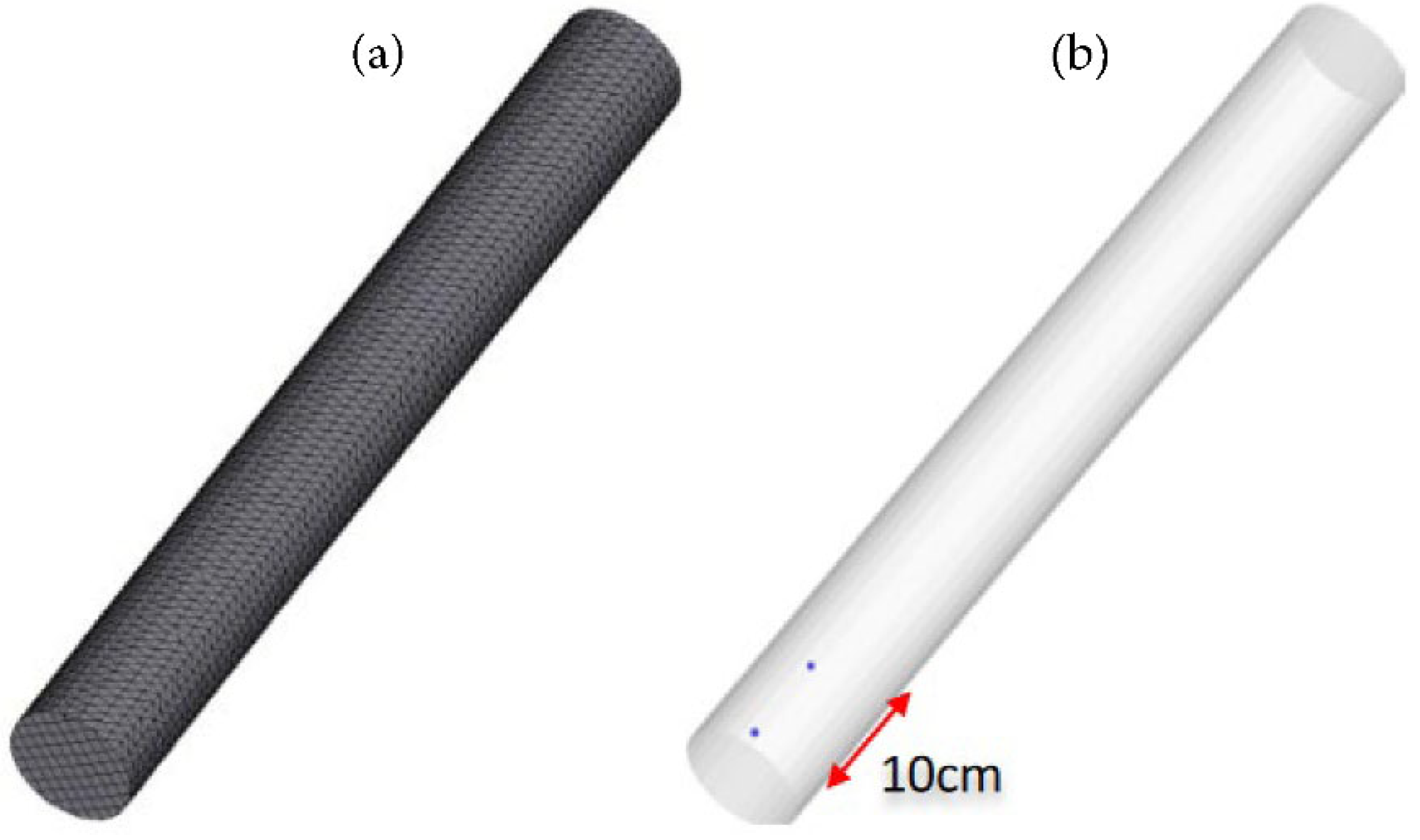
2.2. Cylindrical Fluidized Bed Rig

The cold-flow cylindrical fluidized bed system used is shown in Figure 2. The experiments run with the cylindrical fluidized bed were performed using the zirconia particles discussed in the current study. The initial bed height of the zirconia solid particles was 17 cm. The properties of the zirconia particles are summarized in Table 1. The operational procedure followed in the study and further details of the setup are explained in Chladek et al. [2].

3. CFD Model Description

A 3D model of the classifier was made in Barracuda 17.1. The fluid phase, particle momentum, and fluidizing characteristics were calculated using the Navier–Stokes equations, the Lagrangian description, and the MP-PIC numerical methods [7,8,39], according to the coupling of the gas and particle flow with an interphase drag. The governing equations for the MP-PIC formulation are shown below.

3.1. The Gas Phase

The continuity and momentum equations [40] for the gas phase without reactions and the interface mass transfer in Barracuda [8,40] are

$$\frac{\partial {\theta }_g{\rho }_g}{\partial t}+\nabla \left({\theta }_g{\rho }_g{u}_g\right)=0$$

(1)

and

$$\frac{\partial \left({\theta }_g{\rho }_g{u}_g\right)}{\partial t}+\nabla \left({\theta }_g{\rho }_g{u}_g{u}_g\right)=-\nabla p+\nabla \left({\theta }_g{\tau }_g\right)+{\theta }_g{\rho }_{g}g-F$$

(2)

Here ${\theta }_g, {\rho }_g, u_g,p, {\tau }_g$ are the volume fraction (initial), density, velocity, pressure, and the stress tensor of the gas in the system, respectively. $F$ is the momentum exchange rate per volume between the gas and the particles, $t$ is the time interval, and the $g$ is the gravitational acceleration.

The rate of momentum transfer between the fluid and solid phases per unit volume [8,9] is described by

$$F=\iiint f{V}_p{\rho }_p\left[D\left(u_g-u_p\right)-\frac{1}{{\rho }_p}\nabla p\right]d{V}_{p}d{\rho }_{p}d{u}_p$$

(3)

3.2. The Particulate Phase

The dynamics of the particle phase are described by the particle distribution function, defined by O’Rourke and Snider [41] as $f\left(m_p,u_p,{\rho }_p,x,t\right)$. Here $m_p$ is the particle mass, $u_p$ is the particle velocity, ${\rho }_p$ is the particle density, and $x$ is the particle position. The time evolution of $f$ is obtained by solving a Liouville equation for the particle distribution function [8]:

$$\frac{\partial f}{\partial t}+\nabla \left(f{u}_p\right)+\nabla u_p\left(fA\right)=0$$

(4)

3.2.1. Acceleration Model

The latest particle acceleration model in the MP-PIC method $\left(A\right)$ [8] is given in Equation (5). This is the most common particle acceleration model used in Barracuda, but the acceleration model is different when the blended acceleration model (BAM) [41] is enabled in the calculation. The BAM is explained below.

$$\frac{\partial f}{\partial t}+\nabla \left(f{u}_p\right)+\nabla u_p\left(fA\right)=0$$

(5)

The four first terms, from left to right, on the right-hand-side of Equation (5) are the aerodynamic drag acceleration, the buoyant acceleration, the acceleration due to contact forces, and the gravitational acceleration. The fifth term is a collision model recently implemented in MP-PIC [42,43].

$D$ is the aerodynamic drag function, as defined later in Equation (20), whereas $u_g$ and $p$ are the fluid velocity and pressure, respectively. The particle phase mean density, ${\overline{\rho }}_p$, and the mean velocity, ${\overline{u}}_p$, are defined as in Equations (6) and (7), respectively [41]. ${\theta }_p$ is the particle volume fraction, and $g$ is the acceleration due to gravity. τ is an isotropic solid contact stress and defined in Andrews and O’Rourke [7] and Snider [8], as shown in Equation (8).

$${\overline{\rho }}_p=\frac{1}{{\theta }_p}\iiint fmdmd{\rho }_{p}d{u}_p$$

(6)

$${\overline{u}}_p=\frac{1}{{\theta }_p}\iiint fm{u}_{p}dmd{\rho }_{p}d{u}_p$$

(7)

In the Barracuda model, particle interactions are modelled using a computationally efficient particle stress function. The particle normal stress $\tau$ [8] is a function of the particle volume fraction ${\theta }_p$.

The particle normal stress $\tau$ is [7,8],

$$\tau \left({\theta }_p\right)=\frac{10P_s{\theta }_p{}^{\beta }}{\max \left[{\theta }_{cp}-{\theta }_p,\epsilon \left(1-{\theta }_p\right)\right]}$$

(8)

Here, $P_s$ is a constant with units of pressure, ${\theta }_{cp}$ is the particle volume fraction at close pack, β is a constant with a recommended value between 2 and 5, and ε is a very small number. The original expression by Harris and Crighton [44] was modified by Snider to remove the singularity at close pack, by adding the ε expression in the denominator. Values for the stress model constant, including the close pack volume fraction must be specified in the Barracuda model.

In the present study, the close pack volume fraction is used as 0.6, and the default values 1 Pa, 3, and ${10}^{-8}$ are used for $P_s, \beta ,$ and $\epsilon$, respectively.

${\tau }_D$ is the damping time due to inelastic particle collisions, defined by O’Rourke and Snider [41] in the following equation, which is valid at near equilibrium conditions:

$${\tau }_D=\frac{\sqrt{3\pi }}{16}\frac{ r^{32}}{{\theta }_p\sigma }\left(\frac{1}{g_0\left({\theta }_p\right)\eta \left(1-\eta \right)}\right)$$

(9)

$g_0\left({\theta }_p\right)$ is the radial distribution function [41],

$$g_0\left({\theta }_p\right)=\frac{{\theta }_{cp}}{{\theta }_{cp}-{\theta }_p}$$

(10)

• ${\theta }_{cp}$ is the close pack volume fraction.
• $\sigma$ is the mass-weighted standard deviation of the particle velocity distribution, and defined as [41]

  $$\sigma =\sqrt{\frac{1}{{\overline{\rho }}_p{\theta }_p}\iiint fm{\left(u_p-{\overline{u}}_p\right)}^{2}dmd{\rho }_{p}d{u}_p}$$

  (11)
• $\eta$ is a parameter depending on the particle material coefficient of restitution $e_p$, and $\eta$ is defined as [41]

  $$\eta =\frac{1+e_p}{2}$$

  (12)

The Sauter mean radius $r^{32}$ [41] is given as

$$r^{32}=\frac{\iiint f{r}^{3}dmd{\rho }_{p}d{u}_p}{\iiint f{r}^{2}dmd{\rho }_{p}d{u}_p}$$

(13)

where the particle radius $r={⌈m/\left(4/3\pi {\rho }_p\right)⌉}^{1/3}$.

3.2.2. Blended Acceleration Model

The blended acceleration model (BAM) aims to improve the predicted fluidization behavior for polydisperse particles of different sizes or densities. BAM can calculate the forces between particles in closely packed polydisperse granular beds, as well as the relative motion. Fluidization simulations tend to show a higher degree of particle segregation than that observed in experiments, and this can be avoided by using BAM. With the BAM model, individual particle accelerations are a blend between the particle acceleration of the original MP-PIC method, appropriate for rapid granular flows, and an average particle acceleration applied to closely packed granular flows. As a result, particles at, or near close-pack, tend to move together with velocities close to the averaged velocity, due to enduring particle–particle contacts. In dilute regions, particles tend to move independently of each other, due to having less contact with the surrounding particles [41].

The modified particle acceleration, $A_{mod}$, is expressed as

$$A_{mod}=D\left(u_g-u_p\right)-\frac{1}{{\rho }_p}\frac{\partial p}{\partial x}+g+X-\frac{{\overline{u}}_p-u_p}{2{\tau }_D}$$

(14)

• Here $X$ is the modified acceleration due to contact stresses. The modified acceleration is the most important term for the BAM. $X$ is defined as [41],

  $$X=-\frac{1}{{\overline{\rho }}_p{\theta }_p}\nabla \tau +g_1\left({\theta }_p\right)\left[\overline{D}\left(u_g-{\tilde{u}}_p\right)-D\left(u_g-u_p\right)-\left(\frac{1}{{\overline{\rho }}_p}-\frac{1}{{\rho }_p}\right)\nabla p\right]$$

  (15)

Here ${\tilde{u}}_p$ is the drag average particle velocity [41], given as

$${\tilde{u}}_p=\frac{\iiint fmD{u}_{p}dmd{\rho }_{p}d{v}_p}{{\overline{\rho }}_p{\theta }_p\overline{D}}$$

(16)

Here $v_p$ is the relative velocity of the particle with respect to the fluid velocity and $\overline{D}$ [41] is defined as

$$\overline{D}=\frac{\iiint fmDdmd{\rho }_{p}d{v}_p}{{\overline{\rho }}_p{\theta }_p}$$

(17)

$g_1\left({\theta }_p\right)$ is a blended function, and there are two forms of $g_1\left({\theta }_p\right)$, as explained in detail by O’Rourke and Snider [41].

3.3. Drag Models Used in the Study

The seven available drag models in Barracuda were used in the CFD simulations. The aim was to find the most suitable drag model and further validate it against the experimental data, to then use in the classifier simulations. The Reynolds number for the solid particles varied from 10 to 50, depending on the mean particle diameter of the zirconia and steel. The solid volume fraction in the dense zone of the classifier at the operational conditions varied between 0.2 and 0.35.

The drag models calculate a force, $F_p$, acting on a particle. This is a function of the particle mass, fluid velocity, particle velocity, and the drag function:

$$F_p=m_{p}D\left(u_g-u_p\right)$$

(18)

In many models the drag function [45] is dependent on the fluid conditions, the drag coefficient, and the Reynolds number. The particle Reynolds number is calculated as

$$Re=\frac{2{\rho }_g{r}_p\left|u_g-u_p\right|}{{\mu }_g}$$

(19)

In many models, the drag function $D$ is related to the drag coefficient by

$$D=\frac{3}{8}{C}_d\frac{{\rho }_g\left|u_g-u_p\right|}{{\rho }_p{r}_p}$$

(20)

3.3.1. The WenYu Model

The WenYu model [45,46] is based on single particle drag models and depends on the fluid volume fraction ${\theta }_g$ to account for the particle packing. This drag model is appropriate for more dilute systems. The drag coefficient is a function of the Reynolds number, according to the following set of conditions:

$$C_d=\left\{\begin{array}{ll}\frac{24}{Re}{\theta }_g^{n_0}& \hfill Re<0.5 \\ \frac{24}{Re}{\theta }_g^{n_0}\left(c_0+c_{1}R{e}^{n_1}\right)& \hfill 0.5\le Re\le 1000\\ c_2{\theta }_g^{n_0}& \hfill Re>1000 \end{array}\right.$$

(21)

The constants are

$n_0=-2.65$	$\hspace{1em}{c}_0=1.0$
$n_1=0.687$	$\hspace{1em}{c}_1=0.15$
	$\hspace{1em}{c}_2=0.44$

In the WenYu model, the drag function is calculated using Equation (20).

3.3.2. The Ergun Model

The Ergun drag model is valid only for dense bed calculations, as it was developed based on dense bed data. In the Ergun drag model [47,48], the drag function is given by

$$D=0.5\left(\frac{k_1{\theta }_p}{{\theta }_{g}Re}+c_0\right)\frac{{\rho }_g\left|u_g-u_p\right|}{{\rho }_p{r}_p}$$

(22)

In this equation, the constants are

$c_0=2$ is the non-linear coefficient

$k_1=180$ is the linear coefficient

The recommended values by Pitault et al. [49] for $c_0$ and $c_1$ are 1.75 and 150, respectively, but in Barracuda^® those values are 2 and 180. In the Ergun model, many different constants have been used to fit the model to different data sets.

3.3.3. The WenYu/Ergun Model

The WenYu correlation is suitable for more dilute systems [45], and the Ergun equation [47] is suitable at higher packing fractions [40]. WenYu/Ergun is a drag function developed by combining the WenYu and Ergun functions [40]:

$$D=\left\{\begin{array}{cc}D{ }_1& {\theta }_p<0.75{\theta }_{CP}\hfill \\ \left(D_2 - D_1\right)\left(\frac{{\theta }_p - 0.75{\theta }_{CP}}{0.85{\theta }_{CP} - 0.75{\theta }_{CP}}\right)& 0.75{\theta }_{CP}\ge {\theta }_p\ge 0.85{\theta }_{CP}\hfill \\ D_2& {\theta }_p>0.85{\theta }_{CP} \hfill \end{array}\right.$$

(23)

$D{ }_1$ is the WenYu drag function defined in Equation (21), and $D{ }_2$ is the Ergun drag function defined in Equation (22).

3.3.4. The Turton and Levenspiel Model

The Turton and Levenspiel drag model uses the single particle drag function [50], and the model is dependent on the fluid volume fraction:

$$C_d=\frac{24}{Re}{\theta }_g^{n_0}\left(c_0+c_{1}R{e}^{n_1}\right)+\left(\frac{c_2}{1+c_{3}R{e}^{n_2}}\right){\theta }_g^{n_0}$$

(24)

The default values for the constants are

$c_0=1.0$

$c_1=0.173$

$c_2=0.413$

$c_3=16300$

$n_0=-2.65$

$n_1=0.657$

$n_2=-1.09$

The drag function is calculated using Equation (20).

3.3.5. The Richardson, Davidson, and Harrison Model

In the Richardson, Davidson, and Harrison model [51,52], the drag function is calculated using Equation (20), and the drag coefficient is calculated as

$$C_d=\left\{\begin{array}{ll}\frac{24}{Re}& \hfill Re<0.2\\ \frac{24}{Re}+24c_{0}R{e}^{n_0-1}& \hfill 0.2\le Re\le 500\\ c_1& \hfill Re>500 \end{array}\right.$$

(25)

The constants are

$c_0=0.15$

$c_1=0.44$

$n_0=0.687$

3.3.6. The Haider-Levenspiel Model

The Haider-Levenspiel drag model [53] is given as

$$D=\frac{9}{2}\frac{{\mu }_g}{{\rho }_p{r}^2{}_p}{f}_h$$

(26)

$$f_h=1+c_{0}R{e}^{n_0}+\frac{c_1 R{e}^2}{Re+c_2}$$

(27)

The constants are

$c_0=0.14017$

$c_1=0.19197$

$c_2=2682.5$

$n_0=0.6529$

3.3.7. The EMMS Model

The EMMS drag model [54] is given as

$$D=4.5\left(\frac{u_g}{{\rho }_p{r}_p^2}\right)f_e$$

(28)

Here $f_e$ is a function of the Reynolds number, gas volume fraction, and the adjustable coefficients $c_0$ through $c_{14}$ and $n_{\mathrm{o}}$. The default coefficient values used in the EMMS model based on Yang et al. [54] are given as

$$f_e=\left\{\begin{array}{ll}\frac{1}{18{\theta }_g}\left(c_o\frac{{\theta }_p}{{\theta }_g}+c_{1}Re\right)& \hfill {\theta }_g<0.74 \\ \left(c_2+c_{3}R{e}^{n_o}\right)\omega & \hfill {\theta }_g\ge 0.74 and Re<1000\\ c_4\frac{Re}{24}\omega & \hfill {\theta }_g\ge 0.74 and Re\ge 1000 \end{array}\right.$$

(29)

$$\omega =\left\{\begin{array}{ll}{c}_5+\frac{c_6}{4{\left({\theta }_g+ c_7\right)}^2 + c_8}& 0.74\le {\theta }_g\le 0.82 \hfill \\ c_9+\frac{c_{10}}{4{\left({\theta }_g + c_{11}\right)}^2 + c_{12}}& 0.82<{\theta }_g\le 0.97\hfill \\ c_{13}+c_{14}{\theta }_g& 0.97<{\theta }_g\le 1 \hfill \end{array}\right.$$

(30)

The default constants in the model are given in

Table 2. Default model constants for EMMS model used in Barracuda^® 17.0.

Model Constants
$c_0=150$	$c_5=-0.576$	$c_{10}=0.0038$
$c_1=1.75$	$c_6=0.0214$	$c_{11}=0.7789$
$c_2=1.0$	$c_7=0.7463$	$c_{12}=0.0040$
$c_3=0.15$	$c_8=0.0044$	$c_{13}=-31.8295$
$c_4=0.44$	$c_9=-0.0101$	$c_{14}=32.8295$
		$n_0=0.687$

.

3.3.8. Drag Model Summary

Each drag model was validated for different data sets and their validity is only confirmed for the corresponding conditions.

Table 3. Information about the drag models available in Barracuda^® 17.1.

Model Name	Particle Type Used for Validation	Condition of the Solid Concentration in the Gas Phase	Other Conditions
WenYu	Geldart B	Dilute	$D$ is calculated by Equation (20); the $C_d$ calculation depends on $Re$.
Ergun	Geldart B	Dense
WenYu/Ergun	Geldart B	Dilute and dense	$D$ calculations are based on the ${\theta }_p$ value
Turton and Levenspiel	Geldart B	Dilute	$D$ is calculated by Equation (20); the model is dependent on ${\theta }_g$.
Richardson, Davidson and Harrison	Geldart A and B	Dense	$D$ is calculated by Equation (20).
Haider–Levenspiel	Geldart A and B including non-spherical particles	Dilute
EMMS	Geldart A	Dilute	$D$ is calculated by Equation (20); the model depends on both ${\theta }_g$ and $Re$; suitable for fast fluidization conditions.

shows a summary of the conditions where the different drag models can be used.

3.4. Computational Model, Mesh, and the Geometry

The geometries for the CFD simulations were made in Sold Works^® and later imported to Barracuda VR^® as a STL file. Computational mesh was developed in Barracuda using the inbuilt meshing tool, and recommendations [51] from the CPFD software^® were used. All input parameters for each CFD simulation, including the boundary conditions, were defined with respect to the corresponding experiment. An HP Zbook 15 GS workstation laptop with Processor: Intel^® Core (TM) i7-8850H CPU @ 2.60GHz, 2592 Mhz, 6 Core(s), 12 Logical Processor(s) with 32GB RAM, was used for the simulations. Each case was simulated for 120 to 240 s depending on the superficial gas velocity and particle mass flow rate. It took approximately 24 h to complete each of the simulations. The time taken for the steady state was previously studied for similar cases, and it was observed as approximately 10–30 s.

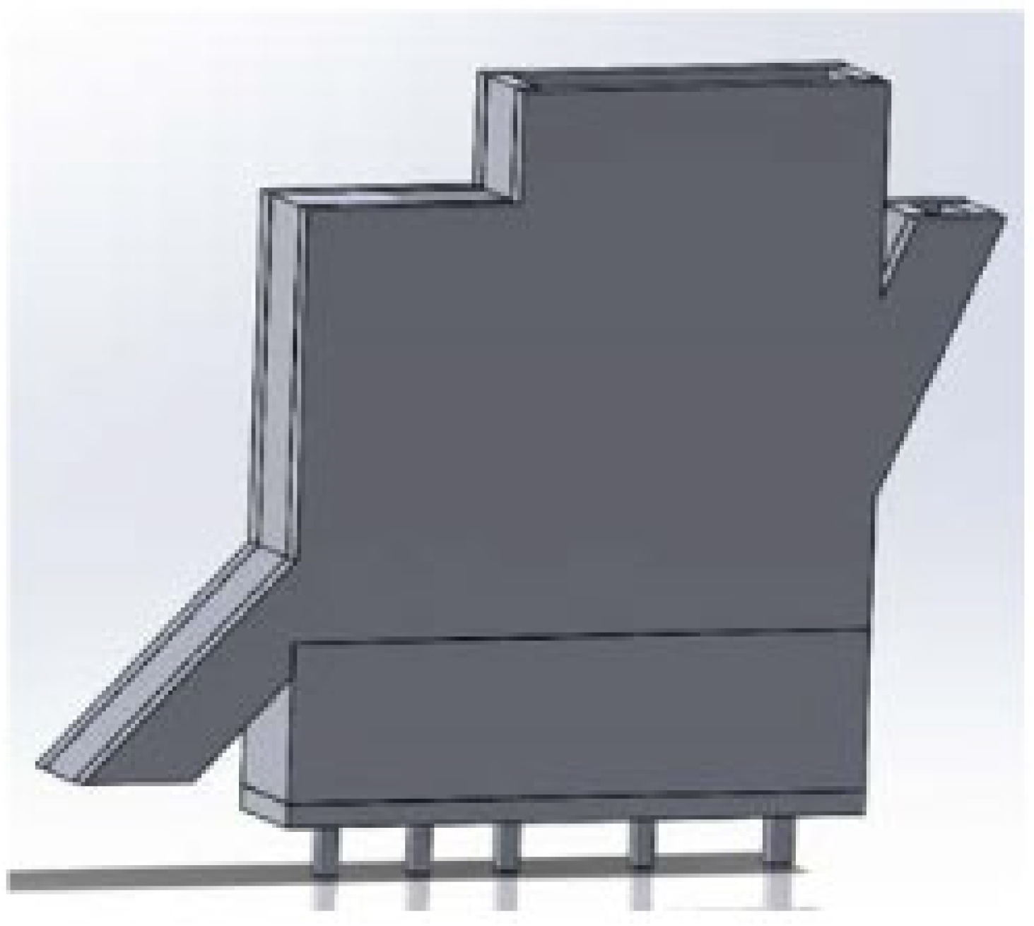
3.4.1. Fluidized Bed Classifier

A cut cell meshing technique was used in Barracuda to model the complex geometries with a Cartesian grid [34]. In this work, it was important to include small details inside the geometry, such as the compartment walls and baffles, see Figure 3 (3D view of the complete classification chamber is shown in Figure 4). Owing to this, a mesh was created with a relatively high number of control volumes, while keeping the normalization factor (aspect ratio of bigger and smaller cells) stable along the X, Y, and Z coordinates. A detailed view of the grid for the solid classifier is shown in Figure 5a. The grid has 77,616 cells.

Boundary conditions of the solid particle inlet, bottom outlet, and air inlets for the five compartments of the classifier were defined with a flow boundary condition. The top outlet was defined as a pressure boundary with the particle outflow, see Figure 5b.

The experiments were performed at ambient temperature (20 °C) and pressure (1 atm); thus, the simulations were done under the same conditions. The close pack volume fraction was set to 0.6, and the maximum momentum redirection from collision was 40%. Other important parameters regarding the particle-to-wall interactions were the normal-to-wall momentum retention, the tangent-to-wall momentum retention, and the diffuse bounce; and these were set to 0.3, 0.99, and 2, respectively.

The drag models were changed in each simulation, as shown in

Table 4. Experimental and CFD simulated cases.

Case No.	Zirconia (wt%)	Steel (wt%)	Solids Feed (kg/s)	Solids Loading (kg/kg)	Drag Modelled Used
1	0	100	0.57	19	WenYu, Ergun, WenYu-Ergun, EMMS
3			1.39	46
23			2.17	73
9	100	0	0.14	5	WenYu, Ergun, WenYu-Ergun, EMMS
4			0.38	13
13			0.59	20
27	28	72	0.22	7	WenYu, Ergun, WenYu-Ergun, Turton-Levenspiel, Richardson-Davidson-Harrison, Haider-Levenspiel, EMMS
28			0.55	18
30			1.06	35
8			1.57	52

, and the default values for the coefficient were used. The sphericity of the particle was assumed to be 0.8, based on examination of the micrographs provided by Chladek et al. [2]. A time step of 0.001 s was selected, and each simulation was run for 100 s. A pseudo steady state was typically reached after around 30 s. This was found by monitoring the accumulated mass vs. time throughout the simulation.

3.4.2. Cylindrical Fluidized Bed Rig

The geometry used for the CFD simulations of the cylindrical lab rig is shown in Figure 6. A three-dimensional cartesian coordinate system was used to describe the vertical cylindrical bed with a diameter of 84 mm and a height of 1.2 m (0.3 m shorter than the actual height, in order to reduce the computation time). The computational grid is shown in Figure 6a. The mesh size was 6.4 × 6.4 × 6.4 mm³, and the number of control volumes was around 25,000. In the present study, the close pack volume fraction used was 0.6. Atmospheric air at room temperature was used as the fluidization medium.

The simulation was run for 30 s for each air flow rate. The same simulation procedure was followed as in the study by Chladek et al. [2]. The total pressure was monitored at positions 2.5 and 12.5 cm above the distributor plate, i.e., at the same positions as in the experiments (see Figure 6b). Transient data were recorded each 0.1 s.

The combined WenYu/Ergun drag model was used for simulations with the cylindrical bed. The coefficient k₁ was set to different values, and the simulation results were compared with experimental values. The following values for k₁ were tried: 180 (default value), 70, 50, 47, and 35.

The pressure-drop over the particle bed (see Figure 2) during the last 5 s of each simulation was averaged. It was assumed that a pseudo-steady state was reached after 15 to 25 s. This assumption was made based on previous simulations under similar conditions.

4. Case Definitions for Experiments with the Fluidized Bed Classifier

One of the requirements from the experimental study was to identify the combination of operational settings that would give a good classification efficiency and a high capacity (throughput). Experimental results from 40 different cases were reported previously [1], and in the present study, the results from 10 of these cases were used for comparison with the CFD predicted results, see Table 4. For practical reasons, the case numbers from the previous publication [1] were also used in the present work.

Six of the cases were associated with pure particles fed at three different solids loading values (solids loading is the mass fraction between the solids and gas feeds). The remaining four cases covered four different solids loading values when the feed was a mixture of zirconia and steel. In all cases, the air flow rate was 0.03 kg/s. The superficial air velocities in each compartment are shown in

Table 5. Superficial air velocity in each compartment.

Compartment	1	2	3	4	5
Air Velocity [m/s]	1.1	1	1.4	1.9	2

.

5. Results and Discussion

As previously mentioned, a detailed discussion about the experimental studies was reported elsewhere [1]; hence, the focus of the present work was to analyze the capabilities of Barracuda to model the behavior of the novel classifier.

Figure 7 shows the classification results from the experiments and corresponding CFD simulations with pure steel particles. The CFD predictions from different drag models shown in the Figure 7 are in relatively good agreement with the experimental results for lower solids loading values (<46 kg/kg). When the solids loading was as high as 73 kg/kg, only the simulation with the Ergun drag model agreed with the experimental results. These CFD predictions agree with the conclusions made by Chladek et al. [2]; i.e., the Ergun drag model predicted almost the same minimum fluidization velocity as observed in the experiments.

However, in the above mentioned study [2], the default drag models available in Barracuda failed to predict the minimum fluidization velocity of zirconia particles. The WenYu drag model gave the best prediction, but still had a deviation of around 50%.

Figure 8 shows the loss of zirconia particles via the bottom of the classifier as a function of the solids loading. Since zirconia is the lighter component in the proposed particle mixture, it should end up as the top product. However, the results from the cold-flow experiments revealed that a large fraction of the zirconia particles ended up in the bottom product as well. Moreover, the zirconia loss was highly underpredicted by the CFD simulations. The reasons for this could be associated with the particle-to-particle interactions and/or particle-to-wall interactions. The underprediction may also have been due to the drag models. Several different drag models available in Barracuda were used in the simulations, and results the from four of those simulations (with four different drag models) are shown in Figure 8. Larger deviations were observed with the other simulations with the remaining drag models.

Considering the particle size distribution (PSD) and the particle density, the zirconia particles used in this study are on the boundary between Geldart A and B particles. Fluidization experiments performed with the same particles showed that they behaved more like Geldart A than Geldart B particles, considering the typical behavior of such particles [55]. In Geldart A particles, the interparticle forces are higher than in a Geldart B particles. The drag models vary in their functional form, and the influence of the interparticle forces on the effective gas-solid drag is not captured [56]. Most of the available drag models are validated for coarse Geldart B particles, and customization is needed for Geldart A particles at similar flow conditions.

The classifier was also simulated with a mixture of steel and zirconia particles, as shown in Table 4. Figure 9, Figure 10, Figure 11 and Figure 12 show the CFD predictions with the different drag models. The losses were calculated as a percentage of the mass for each particle type in the feed.

The model to the far right in the figure is a combination of the Wen/Yu and Ergun models tested in the present study. In this model combination, the WenYu model is used for zirconia and the Ergun model is used for steel particles.

The CFD predictions with the EMMS drag model totally failed to predict the classification. This could be because the classifier is a dense bed with Geldart A and B particles, while the model is intended for simulating dilute Geldart A particles with a fast fluidization regime.

The Turton and Levenespiel model was developed for the determination of terminal settling velocity and drag coefficient for settling spheres. This is a single particle model [50] and dependent on the fluid volume fraction. Hence, it is not surprising that this model was not able to capture the classifier flow phenomena. The Haider and Levenspiel model was also developed from the same basic principles, but it is validated for non-spherical particles as well. Accordingly, neither of these models could make a good prediction for the current case.

The Richardson, Davidson, and Harrison model was developed to study bubble behavior in gas–solid fluidized beds. Nevertheless, the model was not capable of predicting the particle loss in the present work. As reported in the literature [57], even with bubbling beds, this model fails to predict the mushroom shape of the bubbles usually created in fluidized beds.

It was observed that the prediction of the particle loss was not that poor when using the Ergun model and the WenYu/Ergun model. The combined model, which uses Ergun for the steel particles and WenYu for the zirconia particles, also gave quite good predictions, but this model also had deviations from the experimental values that were not acceptable for zirconia particles.

All the drag models overpredicted the classification efficiency and calculated very low steel and zirconia losses compared to the actual values. Most of the drag models managed to predict a decrease in classification efficiency with an increased solids loading, but all of them overpredicted the classification efficiency. The results indicated that Barracuda^® cannot make accurate predictions for these types of particles under the conditions prevailing in a classifier.

In addition to the drag models, the values for packed bed volume fraction, normal-to-wall momentum retention, tangent-to-wall momentum retention, and diffuse bounce influence the model prediction of the classification process. Further investigation of these coefficients could possibly improve the results from the Barracuda^® simulations.

As explained in a previous study [1], a rotary valve was used in the experiments, to control the flow rate of the solid feed to the classifier. A slugging effect at the particle feed was observed, due to the function of the rotary value. This happened when each of the chambers in the rotary valves was releasing particles into the feeding channel while it was rotating.

Owing to this issue, the solids feeding rate was not constant and became a slug flow. Even at lower solids loading conditions, this slugging effect creates a periodic high solids loading condition inside the classification chamber, which leads to a lower classification efficiency. This effect becomes worse at very low solids feed rates, as the rotary valve then rotates at an extremely low rpm. This feed rate behavior was not implemented in the Barracuda^® simulations, and this could have been a possible reason for the deviation between the predictions and the experimental observations.

Figure 13 shows a visual comparison of the flow behavior from the experiments and the CFD simulations for different solids loading values. The Barracuda simulations were done by using the WenYu drag model for zirconia particles and the Ergun drag model for steel particles. The figure clearly shows that the flow behavior in the simulated classifier was very similar to the flow behavior in the actual classifier. It also shows the conversion from a dilute bed into a dense bed with the increase in solids loading.

Both experiments and simulations visualized the streams of zirconia particles leaving from each compartment of the classifier flowing towards the top outlet. In this respect, there was apparently no significant difference between the case numbers, even though the solids loading was increased from 7 to 52 kg/kg.

Most probably, the classifier was overloaded in the cases with the higher solids loading, so that the carrying capacity of the fluidization air was no longer sufficient. As a consequence, a large amount of zirconia ended up in the bottom product. The top left corner of the classifier was filled with a dense particle cloud in Case 8, and the particles accumulating in this area were more likely to be routed towards the bottom outlet than the top outlet, due to the geometric shape of the classifier.

The left upper wall section shown in the black circle in Figure 13 (Case 27) negatively affected the classification process. It was observed in the experiments that a considerable fraction of the zirconia particles bounced back into the dense particle bed after hitting the left upper wall. Most of these particles ended up in the bottom product, as the bottom particle outlet was very close to this part of the geometry.

Another observation was that, even if the particles were in free fall into the classifier through the elevated feeding channel, the horizontal velocity was high and there were no barriers to stop or slow down the corresponding solids flow moving from the inlet to the bottom outlet.

This momentum of the particles reduced the residence time of the particles and had a negative effect on the classification efficiency. There could be a large number of lighter particles trapped inside the dense phase, and these will not have enough time to escape into the freeboard. According to Kunii [55], during fast fluidization, the particles move up or are sent back to the dense phase, depending on the particle size and density. This occurs in the freeboard. Hence, the process in the freeboard area determines whether the particles leave via the top outlet or the bottom outlet. This means, the residence time should be long enough to move each particle into the freeboard for an efficient classification.

Another important factor for efficient classification is to use a taller freeboard than the transport disengaging height (TDH) [55], which means that increasing the height of the classifier could improve the classification. Moreover, barriers in between the solids inlet and the bottom outlet can be used to increase the residence time. The arrangement of these barriers also contributes to sending more particles into the freeboard area. The efficiency may also be increased by placing the bottom outlet slightly above the bottom of the classifier, to avoid the lighter particles moving into the bottom outlet.

Extra internal baffles may help to burst the air bubbles and send the particles to the freeboard area as quickly as possible. This would maintain a lower dense phase height, which facilitates a taller freeboard area. Therefore, increasing the baffle height will not improve the classification efficiency and probably the best thing is to maintain the same height.

Barracuda^® predictions regarding the classification efficiency are not precise, but the predictions of the classifier hydrodynamics were good enough and convenient. Due to this, Barracuda^® was used as a supporting tool for designing and improving the novel classifier.

WenYu/Ergun Drag Model Validation for Fluidization

Based on the current study, it is obvious that the default drag models available in Barracuda^® cannot predict the zirconia particle behavior, even though it almost gives good enough predictions for the behavior of the steel particles. A combination of Ergun and WenYu drag models made slightly better predictions for particles loss. Moreover, it managed to make good predictions of the particle behavior inside the classifier. Based on these predictions it was decided to further validate the combined WenYu and Ergun drag model using basic fluidization experiments performed with the cylindrical fluidized bed system explained in Section 2.2.

The combined WenYu/Ergun drag model gave a wide range of accuracy, by being able to capture the behavior of both dense and dilute particle systems. The predictions of the pressure drop as a function of superficial air velocity at different $k_1$ (see Equation (22)) values are presented in Figure 14.

According to Figure 14, the predictions deviated strongly from the measured values when the default $k_1$ (from Equation (22)) value (180) was used. The reason for this could be that this model was validated with Geldart B particles, and the original model value (150) is not far from the default value (180) used in Barracuda.

Lowering the coefficient value to 70 or 50 gives more accurate predictions, but the predicted stabilized pressure after minimum the fluidization velocity is too high. This value is directly connected to the static pressure head of the particle bed or the weight of the particle bed. It is important that the model can predict this value correctly. A further lowering of coefficient value to 35 gave a too low static pressure head. However, for an intermediate $k_1$ value of 47, both the pressure and minimum fluidization were predicted well. The experimental value and the CFD predictions of the minimum fluidization velocity were 0.015 and 0.016 m/s, respectively. This shows that correct prediction of the fluidization behavior of Geldart A particles is possible with drag model adjustment. The potential drawback is that the adjusted model may be valid only for the current conditions. Further studies are needed to investigate a wider range of air flows, as a further increase of the airflow will increase the pressure drop, since particle entrainment will start. Furthermore, the bed will convert from dense to dilute phase, and the drag model must be validated for that range as well.

Figure 15 illustrates the change of solids volume fraction in the bed with the increased air flow rates. At the minimum fluidization velocity $(u_{mf})$ the weight of the particle bed is balanced by the drag force on the particles, due to the air flow. There is sudden expansion of the particle bed, just after the superficial gas velocity is higher than the minimum fluidization velocity. This phenomenon was clearly illustrated in the simulation with the changes in color and ~4% bed expansion, with around a ~4% void fraction increase.

Following Equation (31), reference [58] explains the connection of the fixed bed pressure drop with the liner coefficient $(k_1)$ of the Ergun drag model. Here $x_{sv}$ is the surface volume diameter (diameter of a sphere having the same volume as the particle) and the other symbols represent the same parameters as discussed in the previous equations.

$$\frac{\left(-∆p\right)}{H}=\left[k_1\frac{\mu }{x_{sv}^2}\frac{{\left(1-{\theta }_g\right)}^2}{{\theta }_g}\right]\left|u_g-u_p\right|+\left[k_0\frac{{\rho }_g}{x_{sv}}\frac{\left(1-{\theta }_g\right)}{{\theta }_g}\right]{\left|u_g-u_p\right|}^2$$

(31)

Equation (31) is only valid for the fixed bed, but the liner effect of the coefficient $k_1$ on the pressure drop is clearly indicated, as represented in the Figure 14 with different $k_1$ values. Rhodes [58], explained that the pressure drop is independent from the relative gas velocity $\left(u_g-u_p\right)$ after the minimum fluidization stage. Assuming this, in the fluidized bed, the entire apparent weight of the particles is supported by the gas flow, and then the pressure drop is given by Equation (32) [58]. In that case, the pressure drop is independent of the coefficient $k_1.$

$$\frac{\left(-∆p\right)}{H}=\left(1-{\theta }_g\right)\left({\rho }_p-{\rho }_g\right)g$$

(32)

As explained in the introduction, the role of the drag model is one of the key factors when modelling the fluidization behavior of a dense gas–solids bed. However, other parameters may also be important; for example, particle-to-wall and particle-to-particle interactions. The model constants related to those phenomena were kept at their default values in this work.

O’Rourke and Snider [48] developed a new acceleration model called the blended acceleration model (BAM) (see Section 3.2.2), and it is claimed to provide improved predictions of the fluidization behavior of non-uniform (polydisperse) particle collections, i.e., particles of differing sizes or densities. BAM was recently implemented in Barracuda^®.

A separate simulation was done by using BAM with the WenYu/Ergun drag model (with $k_1=47$). Figure 16 shows the results compared with those from applying the WenYu/Ergun drag model (with $k_1=47$) without BAM (i.e., one of the lines shown in Figure 16), as well as the experimental results. The bed pressure-drop predictions at superficial air velocities below the minimum fluidization velocity matched the experimental observations when the BAM was enabled. However, the predictions of the stabilized pressure were higher than the experimental values. The simulated minimum fluidization velocity is the same for both cases.

With BAM invoked, the individual particle accelerations are a blend between the particle acceleration of the original MP-PIC method, appropriate for rapid granular flows, and an average particle acceleration that applies to a closely packed granular flows. As a result, particles at or near close-pack tend to move together with velocities close to the averaged velocity, due to enduring particle–particle contacts. In dilute regions, particles tend to move independently of each other, due to having less contact with the surrounding particles [41]. The solids volume fraction of a just fluidized bed is still close to the that of the close-pack bed and tend to move together when BAM is enabled. One of the reasons for this could be that in a real system, air finds open passages to escape, and this leads to a lower stabilized fixed bed pressure drop after the minimum fluidization conditions have been reached. Further investigations of BAM at minimum fluidization conditions of Geldart B and D particles will be useful, to come to a better conclusion.

6. Conclusions

Results from Barracuda^® revealed that adjustments to all the drag models available are needed, to validate against the experimental results. None of these drag models were able to predict the classifier efficiency (with default settings) observed in experiments with steel and zirconia particles. The classification efficiency was always overpredicted in the simulations. However, the simulations with pure particles indicated that the Ergun drag model and the WenYu drag model were both capable of slightly better predictions than the other drag models. It produced good enough predictions for the steel particle loss in classifier simulations, but the predictions for zirconia particle loss were not acceptable.

(1)

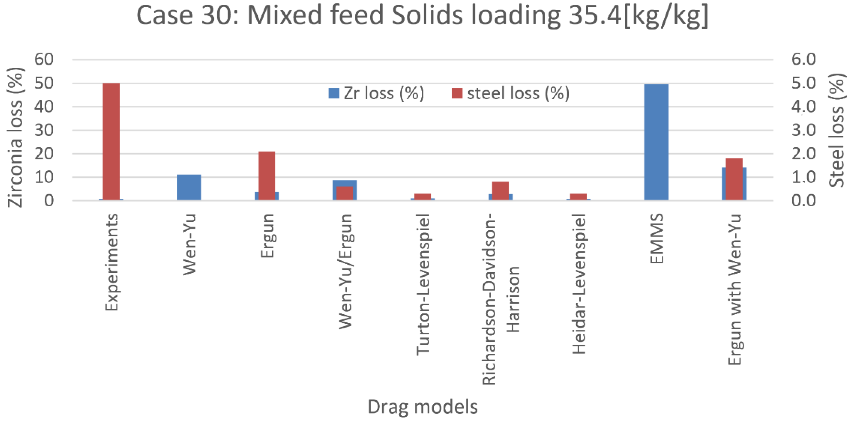
CFD simulations with a particle mixture containing 72 wt% steel and 28 wt% zirconia were best predicted when using the Ergun drag model for steel particles and the WenYu drag model for zirconia particles. Even if the exact particle losses were not predicted rwell, Barracuda^® was able to predict the general gas–solids flow behavior and proved to be a useful tool in the design of the novel classifier. Based on the experimental observations and the CFD simulations, several possible improvements to the classifier design can suggested, as mentioned in Section 5.

(2)

The CFD model was further validated with a Wenyu and Ergun model combination for fluidization experiments done with a cylindrical bed. The results were compared with the CFD simulations run on simulation cases. The Linier coefficient $(k_1)$ of the Ergun drag model, which is used as part of the WenYu and Ergun blended drag model, was altered for the validations. The CFD predictions were matched with experimental data when $k_1=47$. The experimental value and the CFD predictions of the minimum fluidization velocity were then 0.015 and 0.016 m/s, respectively. This shows that correct prediction of the fluidization behavior of Geldart A particles is possible using drag model adjustment. The potential drawback is that the adjusted model may be valid only for the studied air flow rates. Further studies are needed to investigate a wider range of air flows, as a further increase of the airflow will increase the pressure drop, as particle entrainment will start. Graphical observations from bed behavior at minimum fluidization conditions illustrate the real conditions.

(3)

Barracuda^® simulations were performed with the BAM (at $k_1=47)$ model, and the predications for the fixed bed pressure drop were very accurate compared to the experimental observations, but the pressure drop after the fluidization was slightly over predicted. One of the reasons for this could be that in a real system, air finds open passages to escape, and this leads to a lower stabilized fixed bed pressure drop after the minimum fluidization conditions have been reached. With the BAM model, this minimizes the ability of Barracuda to create such open channels in the simulated system, since the particles in a close-pack bed tend to move together when the BAM is enabled.

References

1. Jayarathna, C.K.; Chladek, J.; Balfe, M.; Moldestad, B.M.E.; Tokheim, L.-A. Impact of solids loading and mixture composition on the classification efficiency of a novel cross-flow fluidized bed classifier. Powder Technol. 2018, 336, 30–44. [Google Scholar] [CrossRef]
2. Chladek, J.; Jayarathna, C.K.; Moldestad, B.M.E.; Tokheim, L.-A. Fluidized bed classification of particles of different size and density. Chem. Eng. Sci. 2018, 177, 151–162. [Google Scholar] [CrossRef]
3. Strelow, M.; Schlitzberger, C.; Röder, F.; Magda, S.; Leithner, R. CO2 Separation by Carbonate Looping Including Additional Power Generation with a CO2-H2O Steam Turbine. Chem. Eng. Technol. 2012, 35, 431–439. [Google Scholar] [CrossRef]
4. Reyes-Urrutia, A.; Venier, C.; Mariani, N.J.; Nigro, N.; Rodriguez, R.; Mazza, G. A CFD Comparative Study of Bubbling Fluidized Bed Behavior with Thermal Effects Using the Open-Source Platforms MFiX and OpenFOAM. Fluids 2021, 7, 1. [Google Scholar] [CrossRef]
5. Venier, C.M.; Reyes Urrutia, A.; Capossio, J.P.; Baeyens, J.; Mazza, G. Comparing ANSYS Fluent® and OpenFOAM® simulations of Geldart A, B and D bubbling fluidized bed hydrodynamics. Int. J. Numer. Methods Heat Fluid Flow 2019, 30, 93–118. [Google Scholar] [CrossRef]
6. Soria, J.; Gauthier, D.; Falcoz, Q.; Flamant, G.; Mazza, G. Local CFD kinetic model of cadmium vaporization during fluid bed incineration of municipal solid waste. J. Hazard. Mater. 2013, 248–249, 276–284. [Google Scholar] [CrossRef]
7. Andrews, M.J.; O’Rourke, P.J. The multiphase particle-in-cell (MP-PIC) method for dense particulate flows. Int. J. Multiph. Flow 1996, 22, 379–402. [Google Scholar] [CrossRef]
8. Snider, D.M. An Incompressible Three-Dimensional Multiphase Particle-in-Cell Model for Dense Particle Flows. J. Comput. Phys. 2001, 170, 523–549. [Google Scholar] [CrossRef]
9. Snider, D.M.; Clark, S.M.; O’Rourke, P.J. Eulerian–Lagrangian method for three-dimensional thermal reacting flow with application to coal gasifiers. Chem. Eng. Sci. 2011, 66, 1285–1295. [Google Scholar] [CrossRef]
10. Wang, H.; Qiu, G.; Ye, J.; Yang, W. Experimental study and modelling on gas–solid flow in a lab-scale fluidised bed with Wurster tube. Powder Technol. 2016, 300, 14–27. [Google Scholar] [CrossRef]
11. Vivacqua, V.; Vashisth, S.; Hébrard, G.; Grace, J.R.; Epstein, N. Characterization of fluidized bed layer inversion in a 191-mm-diameter column using both experimental and CPFD approaches. Chem. Eng. Sci. 2012, 80, 419–428. [Google Scholar] [CrossRef]
12. Vashisth, S.; Ahmadi Motlagh, A.H.; Tebianian, S.; Salcudean, M.; Grace, J.R. Comparison of numerical approaches to model FCC particles in gas–solid bubbling fluidized bed. Chem. Eng. Sci. 2015, 134, 269–286. [Google Scholar] [CrossRef]
13. Stroh, A.; Alobaid, F.; Hasenzahl, M.T.; Hilz, J.; Ströhle, J.; Epple, B. Comparison of three different CFD methods for dense fluidized beds and validation by a cold flow experiment. Particuology 2016, 29, 34–47. [Google Scholar] [CrossRef]
14. Fotovat, F.; Abbasi, A.; Spiteri, R.J.; de Lasa, H.; Chaouki, J. A CPFD model for a bubbly biomass–sand fluidized bed. Powder Technol. 2015, 275, 39–50. [Google Scholar] [CrossRef]
15. Liang, Y.; Zhang, Y.; Li, T.; Lu, C. A critical validation study on CPFD model in simulating gas–solid bubbling fluidized beds. Powder Technol. 2014, 263, 121–134. [Google Scholar] [CrossRef]
16. Lim, J.-H.; Bae, K.; Shin, J.-H.; Kim, J.-H.; Lee, D.-H.; Han, J.-H.; Lee, D.H. Effect of particle–particle interaction on the bed pressure drop and bubble flow by computational particle-fluid dynamics simulation of bubbling fluidized beds with shroud nozzle. Powder Technol. 2016, 288, 315–323. [Google Scholar] [CrossRef]
17. Weber, J.M.; Layfield, K.J.; Van Essendelft, D.T.; Mei, J.S. Fluid bed characterization using Electrical Capacitance Volume Tomography (ECVT), compared to CPFD Software’s Barracuda. Powder Technol. 2013, 250, 138–146. [Google Scholar] [CrossRef]
18. Snider, D.; Banerjee, S. Heterogeneous gas chemistry in the CPFD Eulerian–Lagrangian numerical scheme (ozone decomposition). Powder Technol. 2010, 199, 100–106. [Google Scholar] [CrossRef]
19. Alobaid, F. An offset-method for Euler–Lagrange approach. Chem. Eng. Sci. 2015, 138, 173–193. [Google Scholar] [CrossRef]
20. Abbasi, A.; Ege, P.E.; de Lasa, H.I. CPFD simulation of a fast fluidized bed steam coal gasifier feeding section. Chem. Eng. J. 2011, 174, 341–350. [Google Scholar] [CrossRef]
21. Kraft, S.; Kirnbauer, F.; Hofbauer, H. CPFD simulations of an industrial-sized dual fluidized bed steam gasification system of biomass with 8 MW fuel input. Appl. Energy 2017, 190, 408–420. [Google Scholar] [CrossRef]
22. Thapa, R.K.; Frohner, A.; Tondl, G.; Pfeifer, C.; Halvorsen, B.M. Circulating fluidized bed combustion reactor: Computational Particle Fluid Dynamic model validation and gas feed position optimization. Comput. Chem. Eng. 2016, 92, 180–188. [Google Scholar] [CrossRef]
23. Loha, C.; Chattopadhyay, H.; Chatterjee, P.K. Three dimensional kinetic modeling of fluidized bed biomass gasification. Chem. Eng. Sci. 2014, 109, 53–64. [Google Scholar] [CrossRef]
24. Rodrigues, S.S.; Forret, A.; Montjovet, F.; Lance, M.; Gauthier, T. CFD modeling of riser with Group B particles. Powder Technol. 2015, 283, 519–529. [Google Scholar] [CrossRef]
25. Wang, Q.; Yang, H.; Wang, P.; Lu, J.; Liu, Q.; Zhang, H.; Wei, L.; Zhang, M. Application of CPFD method in the simulation of a circulating fluidized bed with a loop seal, part I—Determination of modeling parameters. Powder Technol. 2014, 253, 814–821. [Google Scholar] [CrossRef]
26. Wang, Q.; Niemi, T.; Peltola, J.; Kallio, S.; Yang, H.; Lu, J.; Wei, L. Particle size distribution in CPFD modeling of gas–solid flows in a CFB riser. Particuology 2015, 21, 107–117. [Google Scholar] [CrossRef]
27. Chen, C.; Werther, J.; Heinrich, S.; Qi, H.-Y.; Hartge, E.-U. CPFD simulation of circulating fluidized bed risers. Powder Technol. 2013, 235, 238–247. [Google Scholar] [CrossRef]
28. Shi, X.; Sun, R.; Lan, X.; Liu, F.; Zhang, Y.; Gao, J. CPFD simulation of solids residence time and back-mixing in CFB risers. Powder Technol. 2015, 271, 16–25. [Google Scholar] [CrossRef]
29. Qiu, G.; Ye, J.; Wang, H. Investigation of gas–solids flow characteristics in a circulating fluidized bed with annular combustion chamber by pressure measurements and CPFD simulation. Chem. Eng. Sci. 2015, 134, 433–447. [Google Scholar] [CrossRef]
30. Solnordal, C.B.; Kenche, V.; Hadley, T.D.; Feng, Y.; Witt, P.J.; Lim, K.S. Simulation of an internally circulating fluidized bed using a multiphase particle-in-cell method. Powder Technol. 2015, 274, 123–134. [Google Scholar] [CrossRef]
31. Shi, X.; Wu, Y.; Lan, X.; Liu, F.; Gao, J. Effects of the riser exit geometries on the hydrodynamics and solids back-mixing in CFB risers: 3D simulation using CPFD approach. Powder Technol. 2015, 284, 130–142. [Google Scholar] [CrossRef]
32. Clark, S.; Snider, D.M.; Spenik, J. CO2 Adsorption loop experiment with Eulerian–Lagrangian simulation. Powder Technol. 2013, 242, 100–107. [Google Scholar] [CrossRef]
33. Ullah, A.; Hong, K.; Chilton, S.; Nimmo, W. Bubble-based EMMS mixture model applied to turbulent fluidization. Powder Technol. 2015, 281, 129–137. [Google Scholar] [CrossRef]
34. Ryan, E.M.; DeCroix, D.; Breault, R.; Xu, W.; Huckaby, E.D.; Saha, K.; Dartevelle, S.; Sun, X. Multi-phase CFD modeling of solid sorbent carbon capture system. Powder Technol. 2013, 242, 117–134. [Google Scholar] [CrossRef]
35. Lu, H.; Guo, X.; Jin, Y.; Gong, X.; Zhao, W.; Barletta, D.; Poletto, M. Powder discharge from a hopper-standpipe system modelled with CPFD. Adv. Powder Technol. 2017, 28, 481–490. [Google Scholar] [CrossRef]
36. Chu, K.; Chen, J.; Yu, A. Applicability of a coarse-grained CFD–DEM model on dense medium cyclone. Miner. Eng. 2016, 90, 43–54. [Google Scholar] [CrossRef]
37. Cho, H.; Cha, B.; Ryu, J.; Kim, S.; Moon, I. CPFD Simulation for Particle Deposit Formation in Reactor Cyclone of RFCC. In Computer Aided Chemical Engineering; Iftekhar, A.K., Rajagopalan, S., Eds.; Elsevier: Amsterdam, The Netherlands, 2012; Volume 31, pp. 915–919. ISSN 1570-7946. [Google Scholar]
38. Jiang, Y.; Qiu, G.; Wang, H. Modelling and experimental investigation of the full-loop gas–solid flow in a circulating fluidized bed with six cyclone separators. Chem. Eng. Sci. 2014, 109, 85–97. [Google Scholar] [CrossRef]
39. O’Rourke, P.J.; Zhao, P.; Snider, D. A model for collisional exchange in gas/liquid/solid fluidized beds. Chem. Eng. Sci. 2009, 64, 1784–1797. [Google Scholar] [CrossRef]
40. Gidaspow, D. Multiphase Flow and Fluidization: Continuum and Kinetic Theory Description; Academic Press, Inc.: London, UK, 1993; ISBN 0-12-282470-9. [Google Scholar]
41. O’Rourke, P.J.; Snider, D.M. A new blended acceleration model for the particle contact forces induced by an interstitial fluid in dense particle/fluid flows. Powder Technol. 2014, 256, 39–51. [Google Scholar] [CrossRef]
42. O’Rourke, P.J.; Snider, D.M. An improved collision damping time for MP-PIC calculations of dense particle flows with applications to polydisperse sedimenting beds and colliding particle jets. Chem. Eng. Sci. 2010, 65, 6014–6028. [Google Scholar] [CrossRef]
43. O’Rourke, P.J.; Snider, D.M. Inclusion of collisional return-to-isotropy in the MP-PIC method. Chem. Eng. Sci. 2012, 80, 39–54. [Google Scholar] [CrossRef]
44. Harris, S.E.; Crighton, D.G. Solitons, solitary waves, and voidage disturbances in gas-fluidized beds. J. Fluid Mech. 1994, 266, 243–276. [Google Scholar] [CrossRef]
45. Wen, C.Y.; Yu, Y.H. Mechanics of fluidization. Chem. Eng. Prog. Symp. 1966, 162, 100–111. [Google Scholar]
46. Patel, M.K.; Pericleous, K.; Cross, M. Numerical Modelling of Circulating Fluidized Beds. Int. J. Comput. Fluid Dyn. 1993, 1, 161–176. [Google Scholar] [CrossRef]
47. Ergun, S. Fluid flow through packed columns. Chem. Eng. Prog. 1952, 48, 89. [Google Scholar]
48. Beetstra, R.; van der Hoef, M.A.; Kuipers, J.A.M. Drag force of intermediate Reynolds number flow past mono- and bidisperse arrays of spheres. AIChE J. 2007, 53, 489–501. [Google Scholar] [CrossRef]
49. Pitault, I.; Nevicato, D.; Forissier, M.; Bernard, J.-R. Kinetic model based on a molecular description for catalytic cracking of vacuum gas oil. Chem. Eng. Sci. 1994, 49, 4249–4262. [Google Scholar] [CrossRef]
50. Turton, R.; Levenspiel, O. A short note on the drag correlation for spheres. Powder Technol. 1986, 47, 83–86. [Google Scholar] [CrossRef]
51. CPFD Software. Barracuda Virtual Reactor User Manual; CPFD Software, L.L.C.: Albuquerque, NM, USA, 2017. [Google Scholar]
52. Davidson, J.F.; Harrison, D. Fluidization; Academic Press: New York, NY, USA, 1971. [Google Scholar]
53. Haider, A.; Levenspiel, O. Drag coefficient and terminal velocity of spherical and nonspherical particles. Powder Technol. 1989, 58, 63–70. [Google Scholar] [CrossRef]
54. Yang, N.; Wang, W.; Ge, W.; Wang, L.; Li, J. Simulation of Heterogeneous Structure in a Circulating Fluidized-Bed Riser by Combining the Two-Fluid Model with the EMMS Approach. Ind. Eng. Chem. Res. 2004, 43, 5548–5561. [Google Scholar] [CrossRef]
55. Kunii, D.L.O. Fluidization Engineering; Butterworths: Boston, MA, USA, 1991; ISBN 0-40-990233-0. [Google Scholar]
56. Pannala, S. Computational Gas-Solids Flows and Reacting Systems: Theory, Methods and Practice; Engineering Science Reference: Hershey, PA, USA, 2010; ISBN 978-1-61520-652-0. [Google Scholar]
57. Holdich, R.G. Fundamentals of Particle Technology; Midland Information Technology and Publishing: Shepshed, UK, 2002; ISBN 978-0-95438-810-2. [Google Scholar]
58. Rhodes, M.J. Introduction to Particle Technology, 2nd ed.; John Wiley: Chichester, UK; New York, NY, USA, 2008; ISBN 0-47-198482-5. [Google Scholar]
Figure 1. Cold-flow lab-scale classifier system.
Processes 10 01855 g001
Figure 2. Fluidized bed experimental rig: 1—compressor, 2—ball valve, 3—pressure regulator, 4—mass flow controller, 5—air distribution plate, 6—fluidized bed column, 7—DAQ and LabVIEW, 8—video camera.
Processes 10 01855 g002
Figure 3. Classifier with internal baffles (front plate made invisible).
Processes 10 01855 g003
Figure 4. Classifier with front plate (transparent).
Processes 10 01855 g004
Figure 5. (a) Grid for the CFD simulations. (b) Boundary conditions of the geometry (yellow: pressure boundary conditions, red: flow boundary conditions).
Processes 10 01855 g005
Figure 6. (a) Cylindrical mesh used in the simulations. (b) Transient data points for monitoring the total pressure.
Processes 10 01855 g006
Figure 7. Steel particles exit from top when only steel particles are fed to the classifier.
Processes 10 01855 g007
Figure 8. Zirconia particles exit from the bottom when only zirconia particles are fed to the classifier.
Processes 10 01855 g008
Figure 9. Zirconia and steel loss for Case 27.
Processes 10 01855 g009
Figure 10. Zirconia and steel loss for Case 28.
Processes 10 01855 g010
Figure 11. Zirconia and steel loss for Case 30.
Processes 10 01855 g011
Figure 12. Zirconia and steel loss for Case 8.
Processes 10 01855 g012
Figure 13. Snapshots for four different cases, both from experiments and from Barracuda simulations applying the WenYu model for zirconia and the Ergun model for steel.
Processes 10 01855 g013aProcesses 10 01855 g013b
Figure 14. Change of the pressure drop in the bed with an increased superficial air flow rate.
Processes 10 01855 g014
Figure 15. Snapshots from the simulations at different superficial air velocities.
Processes 10 01855 g015
Figure 16. Change of the pressure drop in the bed with increased superficial air flow rate, with and without BAM.
Processes 10 01855 g016