Uncertainty Propagation Based MINLP Approach for Artificial Neural Network Structure Reduction

Abstract

The performance of artificial neural networks (ANNs) is highly influenced by the selection of input variables and the architecture defined by hyper parameters such as the number of neurons in the hidden layer and connections between network variables. Although there are some black-box and trial and error based studies in the literature to deal with these issues, it is fair to state that a rigorous and systematic method providing global and unique solution is still missing. Accordingly, in this study, a mixed integer nonlinear programming (MINLP) formulation is proposed to detect the best features and connections among the neural network elements while propagating parameter and output uncertainties for regression problems. The objective of the formulation is to minimize the covariance of the estimated parameters while by (i) detecting the ideal number of neurons, (ii) synthesizing the connection configuration between those neurons, inputs and outputs, and (iii) selecting optimum input variables in a multi variable data set to design and ensure identifiable ANN architectures. As a result, suggested approach provides a robust and optimal ANN architecture with tighter prediction bounds obtained from propagation of parameter uncertainty, and higher prediction accuracy compared to the traditional fully connected approach and other benchmarks. Furthermore, such a performance is obtained after elimination of approximately 85% and 90% of the connections, for two case studies respectively, compared to traditional ANN in addition to significant reduction in the input subset.

1. Introduction

Energy producers are globally struggling with the inadequacy of energy resources and energy efficiency problems, which have become even more active in recent years due to COVID-19 pandemics. Another issue to be addressed in today’s world is energy efficiency which is a significant economic growth and prosperity metric. In particular, optimal energy production, distribution, and consumption have vital importance on the economic independence due to the increased energy efficiency. Accordingly, artificial intelligence (AI) and machine learning (ML) have emerged to be nice candidates to improve the efficiency of energy systems without requiring mass investments as opposed to converting all of the energy processing units. Typically, a software can be linked to an energy system and can alter its performance, and thus energy efficiency, using the state-of-the-art approaches on AI and ML.

Artificial neural networks (ANNs) are sophisticated models being able to represent complex relationships between inputs and outputs of a certain system/process. ANNs are data driven and, in particular cases, considered as an alternative to first principles-models because it is challenging to derive and validate such models due to unknown driving forces in the process and lack of spatial measurements [1]. The foundations of ANNs are laid by Mcculloch and Pitts in [2], in which the neural activity working mechanisms are discussed. Significant theoretical advancements have been achieved and these achievements have resulted in a wide range of applications showing promising performance [3,4,5].

Various research activities have also led to different terminologies and applications such as artificial intelligence, machine learning, and deep learning [6,7,8,9]. Murugan and Natarajan designed a dynamic soft sensor to estimate the biomass concentration in a complex pilot plant from easily measurable plant variables (i.e., pH) [10]. Kaur and Kumari used ANNs to detect patterns and risks for diabetes [11]. The applications in mineral processing are discussed in [12]. Moreover, ANN-related methods have found applications in energy economics and finance [13]. In [14], an ANN model is developed to forecast carbon emissions from several macroeconomic indicators such as economic growth. Air pollution forecast studies have used ANNs widely as well [15]. ANNs are also employed in advanced process automation technologies such as stochastic model predictive control [16]. MacMurray and Himmelblau showed the importance of nonlinear and complex processing capability of ANNs in a packed distillation column [17]. Biswas et al. modeled the energy consumption of residential sector through ANNs and showed a good match between prediction and measurements [18]. In addition, there are several successful applications in the literature in terms of using meta-heuristic and multi-verse optimization methods for the improvement of machine learning models in general, resulting in more stable models. Such meta-heuristic based hyper-parameter tuning methods might also improve the capacity of neural networks if applied [19,20]. Ardiansyah et al. used ANNs for the prediction of quality variables and design strategy for an extraction process [21].

Traditional fully connected ANN architectures (FC-ANNs), which are defined by hyper parameters, are composed of single hidden layer in addition to input and output layers. Usually, a trial and error procedure on hyper-parameters is applied until a satisfactory training performance is obtained. Moreover, the number of connections, and the number of tuning parameters increase with the number of inputs, outputs, and neurons. As a result, FC-ANNs suffer from parameter identifiability issues due to multiple solutions, lack of accountable measurements and over parametrization [22]. Overfitting and parameter identifiability problems result in large prediction bounds and therefore poor prediction performance, reducing the performance significantly especially in complex systems. Note that there are some alternative methods to eliminate some of the aforementioned issues using statistical measures [23]. The resulting uncertainty is also addressed in [24] using Bayesian computation.

Group method of data handling (GMDH) [25] develops relatively smaller polynomial models for the approximation of more complex models through elimination of unrelated variables. At the same time, GMDH can be classified as a more sophisticated pruning method. An external selection criterion, which is a nontrivial task to formulate with many different alternatives [26], is used to define the existence or the elimination of a particular network variable. Then, a sorting procedure [27] is applied for the selection of the best architecture among many generated networks. Due to sorting, GMDH can be classified under sequential approaches focusing on the elimination of neurons and inputs. In addition, GMDH does not include covariance of parameters into the objective function.

Dua suggested solving a general mixed-integer optimization problem to eliminate the connections of ANNs during training [28]. Both number of neurons and existence of the interconnections are included in the objective function to be minimized together with the training error. However, this formulation does not consider the parameter uncertainty and the selection of optimum input variables. Resulting problem formulations in the case studies are either mixed-integer linear programs with fixed parameter weights—which are significantly easier problems to solve—or small-scale MINLPs with fixed structures, fixed number of nodes and/or interconnections of the ANNs. Commercially available programming language GAMS (General Algebraic Modeling System) is used to solve the corresponding optimization problems. This significant contribution shows that increased performance can be achieved with fewer number of neurons and connections in ANNs. Similarly, in recent studies, the authors showed that optimal structure detection for ANNs can also be realized using more flexible mixed integer nonlinear programming and piece-wise linear formulations [29,30,31,32].On the other hand, it is vital to state here that none of these formulations include the parameter uncertainty covariance, which is again a critical measure for reliable training and reduced overfitting for not only ANNs but also for almost all types of machine learning applications for regression. Thus, for truly effective structure detection for ANNs, uncertainty effect must also be incorporated into the existing MINLP formulations proposed by the authors.

Another significant aspect of ANN training is the selection of optimal input variables from a complex data set [33]. Usually, the leading signals are not known and the data set contains correlated or redundant variables. In such cases, the optimal selection of input variables becomes an important issue [34], which in turn calls for a robust method to reduce the number of ANN parameters and the input subset selection to provide a more robust identification.

Sun et al. utilized genetic algorithm for automatic design of convolutional neural network architectures for image classification [35]. Benardos and Vosniakos proposed a genetic algorithm to modify the ANN architecture [36]. In a similar fashion, Dua developed a general mixed-integer program to eliminate some connections of ANNs during training [28]. Both the number of neurons and the existence of the interconnections are included in the multi objective function in addition to training error. Yet, these formulations do not consider the parameter uncertainty as a measure of overfitting and the reduction in the input space. On the other hand, it has been shown that a similar performance can be obtained with fewer neurons and connections.

In this study, a novel MINLP (mixed-integer nonlinear programming) formulation is developed for the automatic synthesis and training of an optimal feedforward ANN architecture (OA-ANN). Traditional ANN equations are modified and the training procedure considers the parameter uncertainty to eliminate overfitting. Main contributions of the proposed work are: (i) detecting ideal number of neurons and selection of inputs by introducing binary variables in the MINLP formulation for regression problems through a heuristic yet tailored solution algorithm and (ii) synthesizing the optimal information flow between neurons, inputs and outputs are characterized by introducing binary variable matrices as A_binary and B_binary while minimizing the overfitting criterion by minimizing the parameter covariance as another objective in the optimization for regression problems to account for the tightening the prediction bounds of continuous output variables. To the best of authors’ knowledge such an approach does not exist in the literature. Moreover, to show the potential of improvement for energy systems, a case study about a strong data set on energy consumption predictions is considered in this work.

The paper is structured as follows: In Section 2, the derivation of the ANN (OA-ANN) expressions and the solution algorithm for the corresponding MINLP program are explained. Results of the proposed formulation and comparisons to FC-ANN and literature benchmarks are provided in Section 3. Finally, Section 4 concludes this study.

2. Materials and Methods

A typical feedforward ANN expression is given by:

$$y=f_1\left(A\cdot f_2\left(B\cdot u+C\right)+D\right)$$

(1)

where f₁ and f₂ are output and hidden layer activation functions respectively; A and B are weight matrices; C and D are bias vectors; u is input vector and y is output vector. Note that identity activation function is used in this formulation at the input layer and it is not shown in Equation (1) explicitly. The continuous ANN parameters A, B, C, and D are estimated from preferably high number of samples. The dimensions of those parameters depend on the number of inputs, outputs, and number of neurons (a hyper parameter), which is determined manually before training. In general, as the dimensions get larger, higher number of connections and parameters are introduced, which in turn provides higher capability of fitting to the training data.

The architecture given by Equation (1) represents a FC-ANN which transforms the information in input, u, to the succeeding layers, and eventually to the output vector, y. Addition of a higher number of hidden layers is a straightforward mathematical task as more parameters, connections, and neurons are introduced. This task is in the concept of deep learning, providing useful results in the literature [9,37].

FC-ANNs are traditionally trained through nonlinear optimization using the following objective function:

$$Mi{n}_{A,B,C,D}{\displaystyle {\displaystyle \sum }_{i=1}^N}\Vert f_1\left(A\cdot f_2\left(B\cdot u_i+C\right)+D\right)-y_i\Vert$$

(2)

where u_i and y_i are the ith input and output sample respectively; and N is the number of samples used for the training.

Equation (2) takes the training error into account only and does not consider the parameter identifiability or architecture efficiency issues. However, the practical and structural limitations on the estimation of those parameters are vital in order to increase overall model quality and prediction robustness, and to reduce overfitting. Otherwise, some parameters might have little impact on the output while exhibiting strong correlations among other parameters, making it almost impossible to identify them uniquely [38] despite significant computational load. The outcome of such problem would be the large variance in the ANN predictions due to the parameter uncertainty propagation to outputs and the poor prediction accuracy in the test data once there is a significant difference between training and the test data. In addition, the parameter correlation, which is caused by inefficient model architecture and high number of parameters, results in significant computational load during training or model update as optimization algorithm calculates similar objective function with distinct decision variable values although new data are collected for model correction in real time. An alternative straightforward method to avoid the aforementioned problems would be to include more training data, but is practically not useful mostly once the data are not measured in a distinct data regime. Another alternative is the modification of the model itself either by lumping some parameters, removing some of them by a statistical measure or fixing some of them to a particular value to reduce the parameter correlation, thereby eliminate overfitting. However, this method cannot be considered as automatic and requires significant manual effort.

One of the significant contributions of this work is the integration of the parameter uncertainty propagation together with the proposed MINLP method, which will be discussed later. Parameter covariance matrix is a measure of identifiability in complex models. Based on the Cramer and Rao theorem [39], the inverse of the Fisher Information Matrix (FIM) is a lower bound for parameter covariance matrix:

$$cov\left(\widehat{p}-p^{actual}\right)\ge FI{M}^{-1}$$

(3)

where $\widehat{p}$ is the vector of estimated parameters; $p^{actual}$ the actual value of the parameters; FIM is calculated from:

$$FIM=\frac{1}{{\sigma }^2}J{J}^T$$

(4)

where σ² is the variance of the output error; J is the parameter sensitivity matrix which is evaluated at a particular point. Small eigenvalues of FIM deliver large lower bounds for the parameters, which theoretically means that all parameters cannot be identified uniquely.

The parameter uncertainty can be propagated to the outputs through the traditional error propagation formulation [40]:

$$co{v}_y=J\cdot co{v}_p\cdot J^T$$

(5)

where cov_y is the covariance matrix of outputs; cov_p is the covariance matrix of parameters. Diagonal values of cov_y and cov_p provide an intuitive understanding of the uncertainty since each element is the variance of the corresponding variable. From ANN perspective, once the values in cov_p decrease, corresponding ANN predictions deliver a tighter uncertainty range, resulting in a more robust and reliable prediction generally [41]. As a result, the selected features and connections of the neural network will provide more robust prediction capability.

The modified ANN (OA-ANN) equation to be taken into account as opposed to the standard formulation is given as:

$$y=f_1{\displaystyle (}\left(A\circ A_{binary}\right)\cdot diag\left(P\right)\cdot f_2{\displaystyle (}\left(B\circ B_{binary}\right)\cdot diag\left(U\right)\cdot u+C{\displaystyle )}+D{\displaystyle )}$$

(6)

where $\circ$ is the Hadamard product (element-wise multiplication) operator; A_binary and B_binary are matrices with binary elements, representing the connection existence of hidden layer neurons with the output layer and hidden layer with the input layer respectively; P is a binary vector which represents the existence of neurons; U is a binary vector which represents the input selection; f₁ and f₂ are hyperbolic tangent activation function in this paper. Furthermore, please note that f₁ and f₂ are usually decided before training manually. Even though we propose to use hyperbolic activation functions in this study, suggested framework is also extendable to take into account the type of the activation functions as decision variables.

Mixed-integer programming typically considers the continuous and discrete decisions together to implement an optimization objective subject to constraints. For neural networks, the existence (or non-existence) of the features must be represented as a discrete, binary (0–1) decision variable whereas the corresponding weight values for training are continuous. The training formulation of OA-ANN is an MINLP problem and is given by:

$$\begin{array}{c}Mi{n}_{A,A_{binary},B,B_{binary},C,D,P,U}{{\displaystyle \sum }}^{ }diag\left(co{v}_p\right)+\gamma F\\ s.t.\\ F={\displaystyle {\displaystyle \sum }_{i=1}^N}\Vert f_1{\displaystyle (}\left(A\circ A_{binary}\right)\cdot diag\left(P\right)\cdot f_2{\displaystyle (}\left(B\circ B_{binary}\right)\cdot diag\left(U\right)\cdot u_i+C{\displaystyle )}+D{\displaystyle )}-y_i\Vert \\ A_{binary},B_{binary},P,U\in \left\{0,1\right\}\\ P_{max}⩾{\displaystyle {\displaystyle \sum }_j}{P}_j⩾P_{min}\\ A_{binary,ij}\le P_j\\ B_{binary,ij}\le U_j\\ A_{LB}\times A_{binary,j}\le A_{i,j}\le A_{UB}\times A_{binary,j}\\ B_{LB}\times B_{binary,j}\le B_{i,j}\le B_{UB}\times B_{binary,j}\\ C_{LB}\times P_j\le C_j\le C_{UB}\times P_j\\ D_{LB}\le D\le D_{UB}\\ -4=A_{LB},B_{LB},C_{LB},D_{LB}\\ 4=A_{UB},B_{UB},C_{UB},D_{UB}\end{array}$$

(7)

where γ is a tuning parameter to leverage the multi-objective nature of the problem; P_min is the minimum number of hidden neurons; P_max is the maximum number of hidden neurons. Lower and upper bounds (LB and UB) of continuous variables are shown using subscripts. These lower and upper bounds are set as −4 and 4, respectively.

B_binary,ij is the existence of connection from the jth input as the input information is transferred to i^th hidden layer neuron. Once B_binary,ij is zero, the connection between jth input and ith neuron is eliminated since no information is transferred due to B_binary,ij. Thus, once a particular column of B_binary is zero; no information from the corresponding input can be transferred to the hidden layer. Corresponding U_j is set as zero by the algorithm. Similarly, once the value of P is zero, the information is not transferred through the corresponding neuron, which therefore means that the neuron is eliminated. In parallel, A_binary is the matrix of connection existence between hidden layer and outputs. All these rules are enforced via introducing logic constraints to the formulation in (7).

Equation (7) considers the parameter covariance in the objective function in addition to the training error, where both are highly influenced by the number of parameters and the connections in ANN. From Equation (7), optimal synthesis and training of the corresponding ANN can be employed automatically and simultaneously to obtain OA-ANN. This way, selection of the features and proper conditions are achieved subject to parameter uncertainty manifolds.

There are three types of methods to solve the corresponding mixed-integer type optimization problems, namely evolutionary and derivative-based methods. Two of them can also be combined in a hybrid sense to come up with meta-heuristic method, whose application area has been widening lately [42,43,44]. Typically, rigorous and derivative-based methods may require substantial computational power to solve the MINLP problems to global optimality and is out of the scope of this paper. Yet, it must be here noted that suggested formulations bring about the possibility to obtain global ANN structures when solved with non-convex derivative-based methods. Therefore, in this study, an adaptive, evolutionary, and heuristic solution algorithm together with a local optimization method is suggested for solving the non-convex MINLP proposed in this paper. Please note that similar adaptive methods described in the previous studies can also be utilized to solve the resulting MINLP problems. This method can also be implemented using open-source codes, which is another vital advantage over using many of the commercial solvers.

As mentioned earlier, an adaptive algorithm is selected and the main aim is to divide the original problem into two parts. Accordingly, the solution is obtained through a hierarchical decomposition of binary and continuous decision variables, as outer and inner loops similar to [45,46,47]. Accordingly, the outer loop optimization is an integer programming problem (IP) determining existence of the neurons (P), connections (A_Binary, B_Binary), and selection of input variables (U). After the outer loop is utilized, the inner loop will decide on the optimal weight values for a fixed neural network topology at the current iteration. This decomposition allows faster and effective solution of the original method albeit global optimal cannot be guaranteed.

The outer integer program is given by:

$$\begin{array}{c}Mi{n}_{A_{binary},B_{binary},P,U}{{\displaystyle \sum }}^{ }diag\left(co{v}_p\right)\\ s.t.\\ F\le {\gamma }^{\prime }\\ A_{binary},B_{binary},P,U\in \left\{0,1\right\}\\ A_{binary,ij}\le P_j\\ B_{binary,ij}\le U_j\\ P_{max}⩾{\displaystyle {\displaystyle \sum }_j}{P}_j⩾P_{min}\end{array}$$

(8)

where γ’ is the maximum desired training error. Note that, the multi objective optimization formulation in Equation (7), is further modified and training error term is considered as a constraint to avoid the difficulty in the determination of γ. In practice, larger value of γ in the solution of Equation (7) may result in over simplification of the model, which in turn causes poor training performance.

The inner loop optimization problem is given by:

$$\begin{array}{c}mi{n}_{A,B,C,D}F\\ s.t.\\ F={\displaystyle {\displaystyle \sum }_{i=1}^N}\Vert f_1{\displaystyle (}\left(A\circ A_{binary}\right)\cdot diag\left(P\right)\cdot f_2{\displaystyle (}\left(B\circ B_{binary}\right)\cdot diag\left(U\right)\cdot u_i+C{\displaystyle )}+D{\displaystyle )}-y_i\Vert \\ A_{LB}\times A_{binary,j}\le A_{i,j}\le A_{UB}\times A_{binary,j}\\ B_{LB}\times B_{binary,j}\le B_{i,j}\le B_{UB}\times B_{binary,j}\\ C_{LB}\times P_j\le C_j\le C_{UB}\times P_j\\ D_{LB}\le D\le D_{UB}\\ -4=A_{LB},B_{LB},C_{LB},D_{LB}\\ 4=A_{UB},B_{UB},C_{UB},D_{UB}\end{array}$$

(9)

The inner loop is a nonlinear programming problem (NLP), used typically for training a particular architecture iterate given by Problem (8). The IP given in (8) is solved via the MIDACO solver [48,49], whereas (9) is solved via the open-source IPOPT code [50] on an Intel i5 processor with 8GB of RAM running MATLAB 2020a.

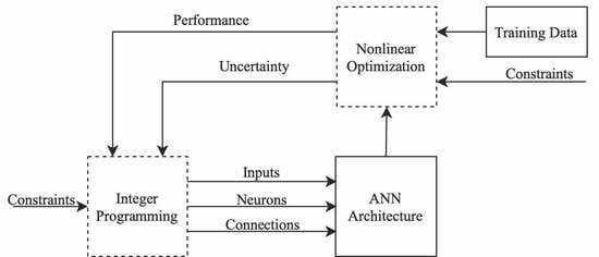
Overall heuristic solution algorithm is shown in Figure 1.

The inner and outer loops are iterated sequentially until the pre-specified convergence (stopping) criterion is reached for the original problem. In this study, this criterion is on the change of the original problem objective, with a value of 0.01. Finally, it is still noteworthy to mention that better solution algorithms can be used while this study mainly focuses on the MINLP approach to combine the feature and structure detection together with the parameter uncertainty prediction for regression problems.

3. Results

This study focuses on two publicly available benchmarks from [51,52]. The performance of the proposed approach is compared to FC-ANN (fully connected) and several other publications which focus on the same dataset. In addition, GMDH (group method of data handling) results are also provided using [53]. We decided to compare the proposed method with the GMDH so as to provide a benchmark using an active subject for pruning.

The performances are evaluated using mean absolute error (MAE), mean square error (MSE), root mean square error (RMSE), coefficient of variation (CV), and mean uncertainty (MU), which are statistical criteria defined in this study, and are calculated from:

$$\begin{array}{c}MU=\frac{{{\displaystyle \sum }}_{i=1}^N\sqrt{\left(co{v}_{y,ii}\right)}}{N}\\ MAE=\frac{{{\displaystyle \sum }}_{i=1}^N\left|y^{prediction,i}-y^{measurement,i}\right|}{N}\\ RMSE=\sqrt{\frac{{{\displaystyle \sum }}_{i=1}^N{\left(y^{prediction,i}-y^{measurement,i}\right)}^2}{N}}\\ CV=\frac{\sqrt{\raisebox{1ex}{${{\displaystyle \sum }}_{i=1}^N{\left(y^{prediction,i}-y^{measurement,i}\right)}^2$}\!\left/ \!\raisebox{-1ex}{$N$}\right.}}{\raisebox{1ex}{${{\displaystyle \sum }}_{i=1}^N{y}^{measurement,i}$}\!\left/ \!\raisebox{-1ex}{$N$}\right.}\end{array}$$

(10)

where y^prediction,i is the prediction of the ith sample output; y^{measurement,i} is the measurement of the ith sample output; N is the number of samples; cov_y,ii is the ith diagonal element of cov_y.

3.1. Case Study 1

The data set collected by the U.S. Census Service on Boston housing prices and the affecting factors are under consideration [54]. The dataset contains 506 different samples of 13 inputs and single output as shown in

Table 1. Variables of the case study 1.

			Mean	Standard Deviation	Minimum	Maximum
Inputs	1	per capita crime rate by town	3.6	8.6	0.0	89.0
	2	proportion of residential zones for lots over 25K sq.ft.	11.4	23.3	0.0	100.0
	3	proportion of non-retail business acres per town	11.1	6.9	0.5	27.7
	4	Charles River dummy variable	0.1	0.3	0.0	1.0
	5	nitric oxides concentration	0.6	0.1	0.4	0.9
	6	average number of rooms per dwelling	6.3	0.7	3.6	8.8
	7	fraction of owner-occupied units prior to 1940	68.6	28.1	2.9	100.0
	8	weighted distances to five Boston employment centers	3.8	2.1	1.1	12.1
	9	index of accessibility to radial highways	9.5	8.7	1.0	24.0
	10	full-value property-tax rate per $10,000	408.2	168.5	187.0	711.0
	11	pupil-teacher ratio by town	18.5	2.2	12.6	22.0
	12	1000 (Bk-0.63) 2 where Bk is the proportion of a particular resident group in town	356.7	91.3	0.3	396.9
	13	% lower status of the population	12.7	7.1	1.7	38.0
Output		Median value of owner-occupied homes in $1000s	22.5	9.2	5.0	50.0

. Randomly selected 50% of the data is used for training and normalized for numerical purposes.

Boston housing dataset is specifically chosen as a case study since it contains relatively low number of samples, and overfitting is highly likely when high number of parameters is introduced. In addition, it has many inputs based on residential and cultural measurements which contain some correlation inherently; and thus, input selection and elimination become an important issue.

Figure 2 includes training and test performances of a FC-ANN containing 10 neurons in the hidden layer. The FC-ANN contains 151 continuous parameters to be estimated. Accurate estimation of such a high number of parameters is theoretically challenging and likely to result in overfitting, considering 253 training samples with 13 inputs.

FC-ANN delivers a relatively better training performance due to high number of connections, neurons, and inputs. On the other hand, a significant performance drop is observed for the test data due to overfitting, in this particular relatively smaller case study. The error bars of the predictions are obtained from (5), using the uncertainties in the parameters after the training. Please note that these measures could represent prediction robustness and reliability. (6) delivers the mean value of the predictions based on the mean parameter values at a particular architecture. Due to probable overfitting in FC-ANN, the prediction uncertainty and error are significantly large, which in practice means predictions might not be reliable.

Solutions of (8) and (9) deliver the OA-ANN, whose performance is shown in Figure 3.

Table 2. Results of case study 1.

		OA-ANN	FC-ANN	[55]	[56]	GMDH
training	MAE	0.050	0.013	-	-	-
	MSE	0.004	0.0003	-	-	0.006
	RMSE	0.067	0.019	-	-	0.078
	RMSE *	3.086	0.849	-	3.369	-
	MU	0.018	0.278	-	-	-
test	MAE	0.058	0.097	-	-	-
	MSE	0.009	0.024	-	-	0.012
	RMSE	0.096	0.155	0.187	-	0.119
	RMSE *	4.331	6.990	-	7.602	-
	MU	0.018	0.195	-	-	-
${{\displaystyle \sum }}^{ }diag\left(co{v}_p\right)$		0.533	27998	-	-	-
Neuron		2	10	-	20	8
Inputs		11	13	13	6	6
Connections		22	151	-	-	65

* Calculated without data normalization.

provides detailed statistical comparisons based on the common measures. The performance increase is obtained through optimal architecture design and training. Note that all OA-ANN test errors and prediction uncertainty range are lower than FC-ANN as shown in Table 2, in this particular case. Corresponding OA-ANN architecture, which does not explicitly demonstrate the bias connections, is shown in Figure 4.

As shown in Figure 4, in this particular case, only two neurons (although maximum ten are allowed) are introduced with the elimination of proportion of non-retail business acres per town and nitric oxides concentration from the input set. Note that there is no connection between the corresponding input and any hidden neuron. In addition, OA-ANN contains a significantly fewer number of connections among variables; for instance, Charles River dummy variable provides information in the calculation of the output variable, through the 1st hidden neuron only. Furthermore, the connection line widths are scaled by the absolute values of the corresponding weight.

The OA-ANN, using fewer network elements, provides a comparable performance with the benchmarks in the literature and GMDH. In [55], an extreme learning machine confidence weighted method is proposed using 79% of the whole data in training. Ref. [56] used 60% of the whole data, and reported radial basis neural network results using different number of neurons. Ref. [57] also refers to various other models and provides a performance comparison on Boston housing dataset with test RMSE^* values between 3.206 and 7.610. In our particular case, OA-ANN has better performance compared to most of the other approaches.

3.2. Case Study 2

Our second case study is related to predicting the electricity consumption of a building. The dataset includes relatively higher number of samples, being with 4208 points, and is directly taken from PROBEN 1 benchmark problem set [52]. The dimension of the input vector is 14 in total as some of the inputs are lumped into each other in the original dataset [58]. The electricity consumption (WBE) is predicted based on year, month, date, day of the week, time of day, outside temperature, outside air humidity, solar radiation and wind speed. The statistical description of the dataset is summarized in

Table 3. Statistical description of case study 2.

	Inputs														Output
Mean	0.1	0.1	0.1	0.1	0.1	0.1	0.1	0.5	0.0	0.0	0.6	0.3	0.1	0.2	0.3
Standard Deviation	0.4	0.3	0.3	0.3	0.3	0.3	0.3	0.3	0.6	1.0	0.2	0.2	0.2	0.1	0.1
Minimum	0.0	0.0	0.0	0.0	0.0	0.0	0.0	0.0	−1.0	−1.0	0.0	0.0	0.0	0.0	0.1
Maximum	1.0	1.0	1.0	1.0	1.0	1.0	1.0	1.0	1.0	1.0	1.0	0.9	1.0	0.9	0.7

.

Performance of the proposed OA-ANN on the prediction of building electricity consumption is compared with fully connected ANN (FC-ANN) and GMDH, and two well-known benchmarks using the same dataset taken from the literature [59]. In [59], the authors used single hidden layer feedforward ANN structure employing hyperbolic tangent activation functions. They introduced identification, additive, and subtractive phases into their training algorithm as opposed to classical methods and sequentially analyzed the effects of the number of inputs and the number of neurons. 70% of the whole data are used for all phases described in the paper. Results showed that reducing the geometry of the ANNs could yield much better test results.

In [60], a hybrid genetic algorithm-adaptive network based fuzzy inference system is proposed to train feedforward artificial neural networks. 70% of the whole data are used for training. This paper also proposes an optimization-based training method and reduces the size of the ANNs using sequential analysis. However, this method is not an automatic and simultaneous design and training method and does not take the covariance of parameters into account.

The proposed method is implemented with 15 maximum number of hidden neurons (P_max), using 70% of the whole data for training. Same training and test dataset, input and neuron numbers are implemented to FC-ANN and GMDH for fair and clear comparison. All results are reported in

Table 4. Results of case study 2.

		OA-ANN	FC-ANN	[59]	[60]	GMDH
training	MSE	0.0026	0.0009	0.008	-	-
	MAE	0.042	0.038	-	-	-
	CV	12	10	12	9.6	11.3
	RMSE	0.051	0.03	0.09	-	0.07
	MU	0.0043	0.015	-	-	-
test	MSE	0.002	0.0043	0.02	-	-
	MAE	0.041	0.06	-	-	-
	CV	9.3	11	13	10	11.1
	RMSE	0.046	0.065	0.14	-	0.069
	MU	0.0044	0.016	-	-	-
${{\displaystyle \sum }}^{ }diag\left(co{v}_p\right)$		2.8	1.2 × 106	-	-	-
Neuron		5	15	4	4	6
Inputs		6	14	10	5	7
Connections		23	241	49	29	55

.

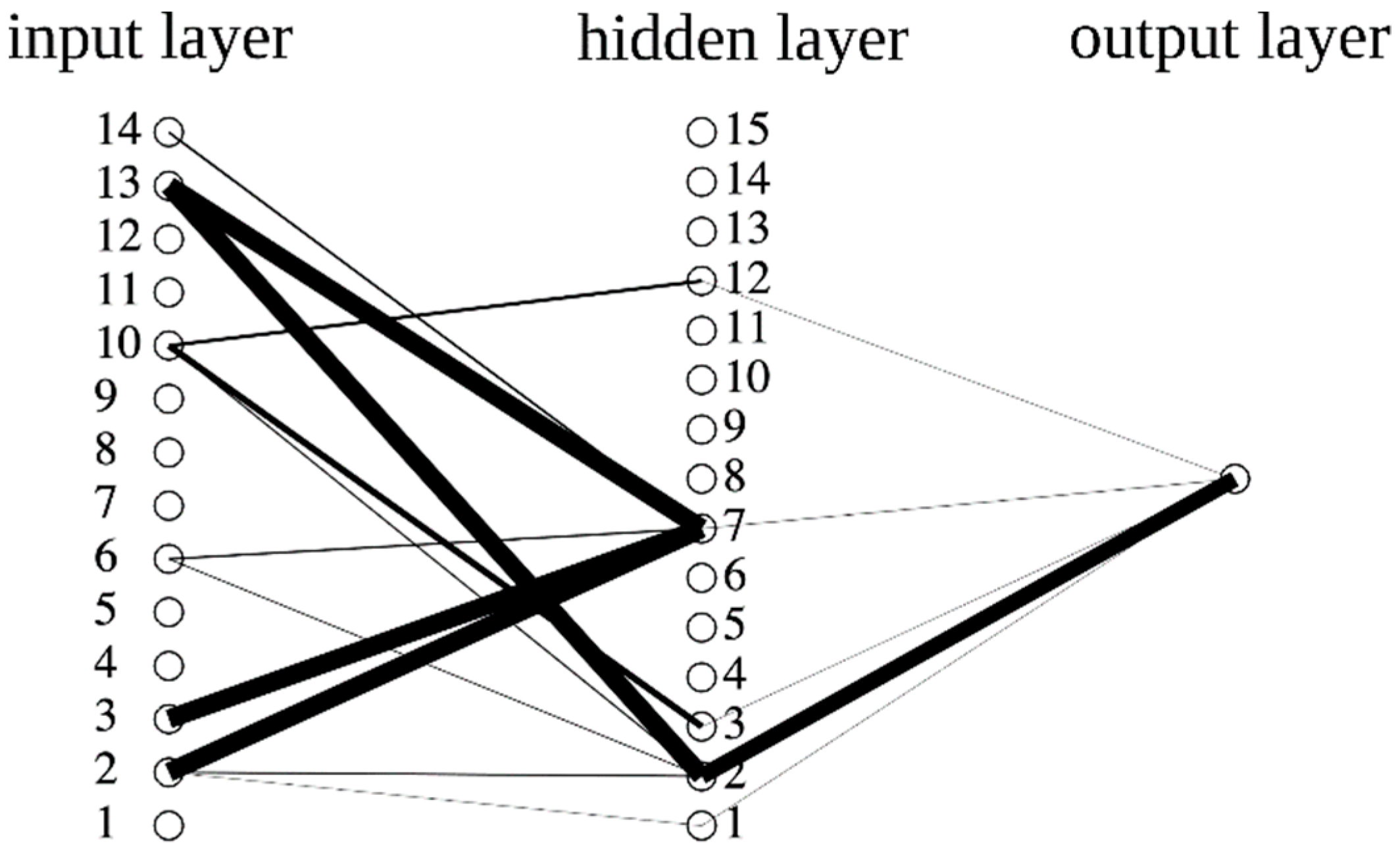
Results for OA-ANN show that the method proposes to use six inputs, being year, month, type of day, temperature, solar radiation, and wind speed.

As shown in Figure 5, in this particular case, 5 neurons (out of 15) are selected. Similar to first case study, the connection line widths are scaled by the absolute values of the corresponding weight.

Table 4 provides detailed statistical comparisons based on the common measures. Coefficient of variation (CV), which is used in other benchmarks, is also included into this case study [60]. Table 4 shows that OA-ANN includes 23 connections among all variables in total, which is significantly fewer than the FC-ANN. Accordingly, OA-ANN exhibits poor training performance than the FC-ANN in all statistical metrics except mean uncertainty. On the other hand, OA-ANN provides better test performance than the traditional FC-ANN in spite of using fewer numbers of inputs, neurons and connections. Such improved prediction quality increase is obtained with almost 90% decrease in the number of connections compared to FC-ANN.

Similarly, the benefit of size reduction and pruning for ANNs in the context of optimization can be observed from [60], whose performance is relatively better compared to other benchmark studies using the same dataset [59]. Even though OA-ANN has poorer training performance compared to [60], OA-ANN exhibits the best test performance among all benchmarks reported in this paper, both in terms of reduced standard deviation and test error. The main reason for this observation is the fact that OA-ANN considers the covariance of the parameters as an optimization metric to be minimized, in addition to the training objective function. As a result, uncertainty regions of the OA-ANN predictions are tightened, as shown in Table 3. This tightening ultimately brings about much fewer values for MU, CV and ${{\displaystyle \sum }}^{ }diag\left(co{v}_p\right)$, which in turn enhances both accuracy and precision of model predictions.

4. Conclusions

This study focuses on the simultaneous optimal architecture ANN design and training algorithm under parameter uncertainty and uncertainty propagation considerations for regression problems; in contrast to traditional approaches where the structure is fixed by predefined hyper parameters based on trial and error procedure. The existence of the connections, the selection of input variables and the determination of the number of hidden neurons together with connection weights are under consideration. The main aim of this formulation is to obtain the optimal ANN structure, and to train this structure with the most dependable input variables considering the parameter identifiability issues to deliver a prediction with lower confidence interval, or to be more precise, uncertainty.

The proposed approach integrates the design and training simultaneously through an MINLP problem which is decomposed for the utilization in successively solved smaller optimization problems, mainly IP and NLP. The MINLP problem involves the training error and the parameter covariance matrix as an uncertainty measure. It also ensures the selection of identifiable set of parameters, resulting in a more robust prediction performance. Furthermore, the MINLP problem includes extra logic constrains for a more efficient solver performance.

The proposed MINLP formulation is comprehensive, sophisticated, and modifiable to other ANN types (i.e., recurrent ANNs, convolutional neural networks). However, similar to many machine learning algorithms, ANNs suffer from nonconvex optimization problem due to nonlinear activation functions and the performance is highly sensitive to initial guess and optimization algorithm, which might deliver local optimum with different ANN weights despite processing same training data. The proposed formulation further increases the complexity of the training problem by introducing binary variables to represent the existence of a particular network element. Such a desirable theoretical superiority calls for mixed-integer optimization algorithms whose global optimum finding capability is still limited with a complex nonconvex problem and require significant computational load due to rigorous formulation. On the other hand, convex MINLP solvers, similar to heuristic optimization algorithms, deliver a local optimum with a significant and computation time increases drastically since all variables are modified simultaneously in the iterations. For such considerations, in this study, a pseudo-decomposition is applied to obtain a satisfactory ANN architecture and performance through computationally favorable heuristic method. The proposed heuristic solution method also suffers from local optimality issues since no explicit modification is implemented to handle nonconvexity related problems. The integer programming stage in the nested algorithm enables the evaluation of any blackbox formulation in the inner loop; but makes the overall solution exposed to failures once the tuning of the corresponding stage optimization problem is poor or not compatible with the inner loop. In addition, the interactions of the layers might bring additional infeasibility problems since there the problems process different constraints. Some linking constraints are introduced to tighten the search space and bring computational efficiency. However, the proposed pseudo-decomposition benefits from rigorous formulations in the inner loop where nonlinear programming is performed with sophisticated mathematical developments including algorithmic differentiation. The development of pseudo-decomposition through using more sophisticated optimization algorithms with a better tuning combined with feasibility cuts and pumps would further increase the computational efficiency, which is under consideration for our future works.

The proposed approach is implemented on two publicly available datasets which are studied extensively in the literature. It is shown that, the current approach provides a better test performance despite increased training error. Finally, the current research activities focus on extending the suggested framework for deep and recurrent neural networks and for synthesizing more efficient neural network-based controller structures.