Unsteady 3D-CFD Simulation of a Large Active Area PEM Fuel Cell under Automotive Operation Conditions—Efficient Parameterization and Simulation Using Numerically Reduced Models

Abstract

Polymer electrolyte membrane fuel cells (PEMFC) are promising devices for securing future sustainable mobility. Their field of application ranges from locally emission-free stationary power generation to propulsion systems for vehicles of all kinds. Computational fluid dynamic (CFD) simulations are successfully used to access the internal states and processes with high temporal and spatial resolution. It is challenging to obtain reliable physical values of material properties for the parameterization of the numerous governing equations. The current work addresses this problem and uses numerically reduced models to parameterize sophisticated transient 3D-CFD models of a commercial PEMFC. Experimental data from a stack test stand were available as a reference for numerical optimization of selected parameters and validation purposes. With an innovative meshing approach, the homogenized channels approach, a reduction of computational cells by 87% could be achieved, thus enabling the unsteady simulation of a 120 s load step with a computational mesh that represents the entire fuel cell geometry with reasonable computational effort. The water formation and the transport processes during the load step were analyzed. The self-humidification strategy of the fuel cell gases was visualized and the uniformity of the simulated quantities was discussed. An outlook on possible future work on efficient parameterization is given.

1. Introduction

Hydrogen will play an important role as an energy carrier in the future. Renewable electrical energy is used to produce it, carbon dioxide-free, by electrolysis from water. Fuel cells convert the hydrogen back into electricity efficiently, and here, polymer electrolyte membrane fuel cells are showing promising performance [1,2]. Not only in stationary applications but also in mobility applications such as buses or truck propulsion systems, this design has been and is being successfully deployed [3,4]. The main advantages of PEMFCs are high efficiency, low operating noise, high startup availability, and high dynamic range [5,6]. The multiphase transport processes in membrane electrode assemblies (MEAs) and the durability and, hence, degradation of PEMFCs in cyclic operation are still areas of research. Transient 3D-CFD simulations with high temporal and spatial resolution and their ability to provide deep insights into internal processes and states accelerate development and reduce the need for prototypes [7,8,9].

The development of simulation models of fuel cells started with the pioneering work of Springer [10] and Bernardi and Verbrugge [11]. During the past years, many models with different dimensionality and physical depth were presented [8,12,13,14,15,16,17,18]. With the increasing computational power, more sophisticated models such as unsteady, non-isothermal, two-phase 3D-CFD models were developed. Many authors reported the use of 3D-CFD PEMFC models with different commercial CFD codes, such as OpenFoam [19], Ansys Fluent/CFX [20,21,22,23], StarCCM+ [24,25], and AVL Fire™ [26].

One of the first 3D multiphase and multicomponent models of PEMFCs was developed by Berning and Djilali [23] and implemented into Ansys CFX (former AEA Technology). Catalyst layers were not fully modeled but were represented by thin interfaces. Their main focus was on the formation of liquid water inside the gas channels and GDLs. Fink et al. [27] presented an unsteady, multiphase, multicomponent and non-isothermal 3D-CFD model which is also used in this work to carry out the CFD simulations.

Some of the authors focused on single-channel models [28,29,30,31,32], but with the increase of computational power, discretizations of the entire geometry [19,21,33,34,35,36,37,38,39] or modeling degradation [27,40,41] have become more common.

Iranzo et al. [21] used the PEMFC model implemented in Ansys Fluent to give a guideline on how to cope with the parameterization challenge of such models. They had experimental data from one polarization curve and tried to fit the simulation results to this data by adjusting the reference exchange current density (RECD) of the cathode catalyst layer (CCL). The remaining parameters were taken from data sheets, literature review, and measurements. The simulation results and measured data showed good agreement with the polarization curve from experimental data. In [35], the simulated liquid water distribution with the CFD model was validated with neutron imaging.

Macedo-Valencia et al. [36] proposed an extension of the Ansys Fluent model by modeling the catalyst layers and membrane with computational cells as well. They simulated a short stack with five cells and an active area of $31.2$ cm${}^2$. Their model was validated against available experimental data of a polarization curve but showed quite high deviations. The parameters of the 3D-CFD model were not perfectly fitted.

With increasing computational power, articles featuring transient 3D-CFD simulations of PEMFCs have been published in recent years. Iranzo and Boillat [42] simulated the unsteady gas transport in the cathode side of a PEMFC during an AC impedance test. Khajeh-Hosseini-Dalasm et al. [43] developed a 3D transient two-phase isothermal model to investigate the time variation of liquid water formation and the gas phase transport under startup conditions. Similarly, Peng et al. [31] developed a transient heat and mass transfer 3D-CFD model to investigate a PEMFC with a dead-ended anode channel. They conducted simulations with and without purging of hydrogen at the anode outlet to show the differences in fuel cell performance. Variations in pressure and relative humidities of fuel and oxidant were investigated. Yan et al. [38] conducted an unsteady 3D-CFD investigation of a serpentine flow field PEMFC to evaluate the effects of serpentine flow field design on the transient characteristics.

Verma and Pitchumani [44] created a transient single-channel model of a PEMFC to study water transport, especially the influence of membrane properties on the behavior during dynamic load changes. They found that current density steps lead to drying of the anode due to increased electroosmotic drag. In [45], the same model was used to conduct a model-based parametric study on the effects of operating parameters during a step change in load. Low inlet gas humidity significantly affects the transient behavior of the fuel cell until a steady state is reached. In [46], they investigated the behavior of the single-channel PEMFC under transient changes in voltage, pressure, and stoichiometry in relation to the power demand of automotive cycles. They also simulated 180 s of the US06 drive cycle and optimized cell potential, inlet pressures, and mass flows to deliver the required performance.

Besides the numerical effort of fully resolved CFD analysis, the question of the parameterization of the transport and Butler–Volmer equations arises. The scatter of experimental data for material parameters of PEMFC models was highlighted by Vetter and Schumacher [47]. Even with accessible data from data sheets of the materials, there is still an uncertainty due to compression of the parts, contact resistances, or its dependence on, e.g., water content and temperature [48]. Moreover, new materials such as ultra-thin reinforced short-side-chain membranes may lack reliable experimental material parameters [49].

Iranzo et al. [21] proposed to use the reference exchange current density as a calibration parameter to fit the simulated data to experimental data. A similar approach was made by Fink et al. [40]. Recently, many authors have developed parameterization strategies for models with reduced dimensionality [50,51,52,53,54]. However, to the authors’ knowledge, there is no work that addresses the efficient parameterization of 3D-CFD models that predict a wider range of steady-state and transient operating conditions.

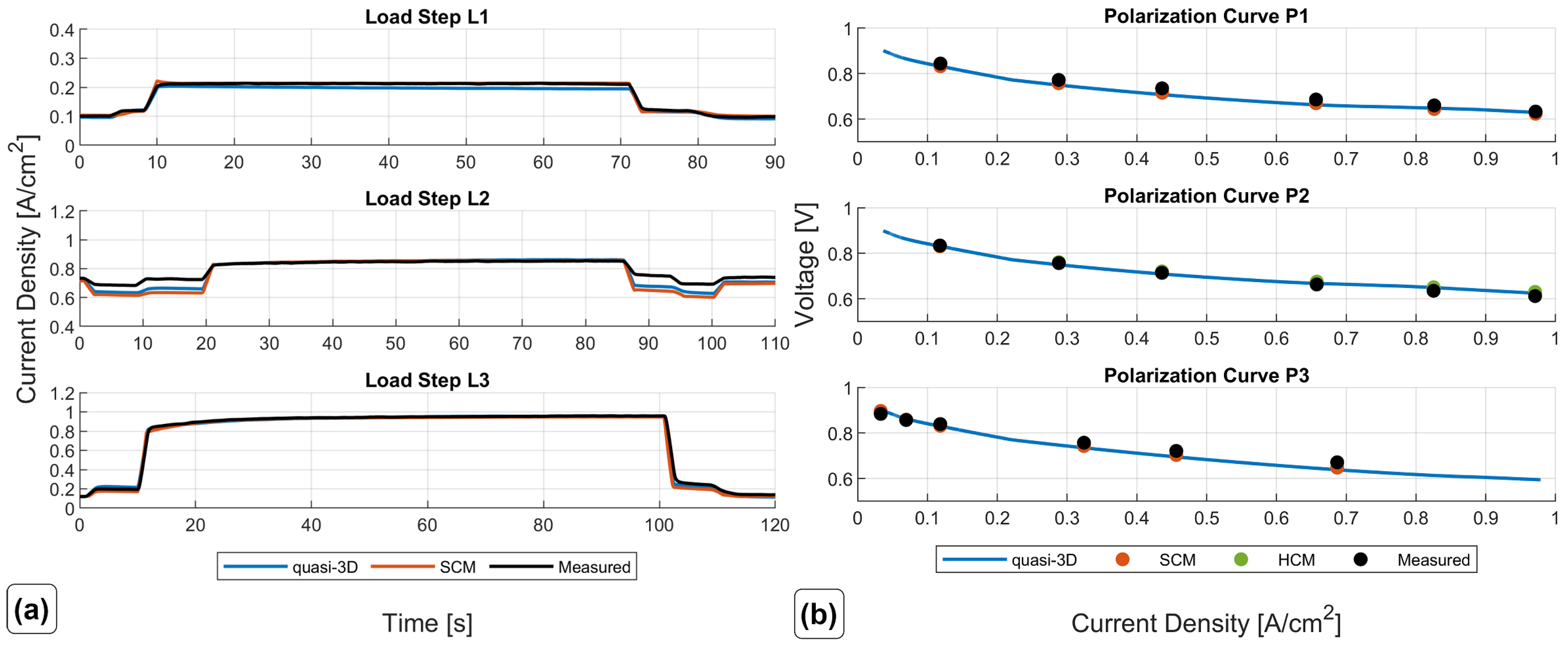
This work is intended to be a guide for efficient parameterization of an unsteady 3D-CFD model for industrial, low temperature PEMFCs with large active area. Using the same approach as in [21,40], the authors of this work had great difficulty in accurately predicting other available experimental data with the fitted RECD. Based on the previous work of the authors [55], numerical optimization methods with the use of numerically reduced models were used to parameterize a 3D-CFD model. For parameterization and validation, measurement results of three load steps and three polarization curves were available, which were measured at the institute’s stack test stand. These data had to be reduced from the stack level to the cell level in order to obtain suitable boundary conditions for the single fuel cell simulations. Therefore, the presented results represented an average large active area fuel cell of a commercial 30 kW PEMFC stack. The experimental data included species mass flows at the inlets, pressures at the outlets, cooling temperatures, and gas humidities at the inlets. The high number of necessary model evaluations of numerical optimization methods were enabled by the use of numerically reduced models, but with very similar physical modeling approaches. With the results from the parameterization process, the transition to CFD was carried out with a single-channel model of the fuel cell. This model provided acceptable accuracy and low simulation times and it enabled the further refinement of parameters for the CFD models. The results show excellent agreement with the measured data, not only with the quasi-3D model but also with the 3D-CFD models. The obtained parameter set was able to predict measured load steps as well as measured polarization curves with minimum deviation.

Despite the reduction from stack to cell level, an alternative meshing strategy is presented to enable the transient 3D-CFD simulation of large active area fuel cells with reasonable computational effort. This approach uses porosity sections instead of the original flow field and steers the flow into the desired direction with anisotropic permeabilites. The number of computational cells could be reduced by a factor of 87% compared to a computational mesh with fully resolved gas channels.

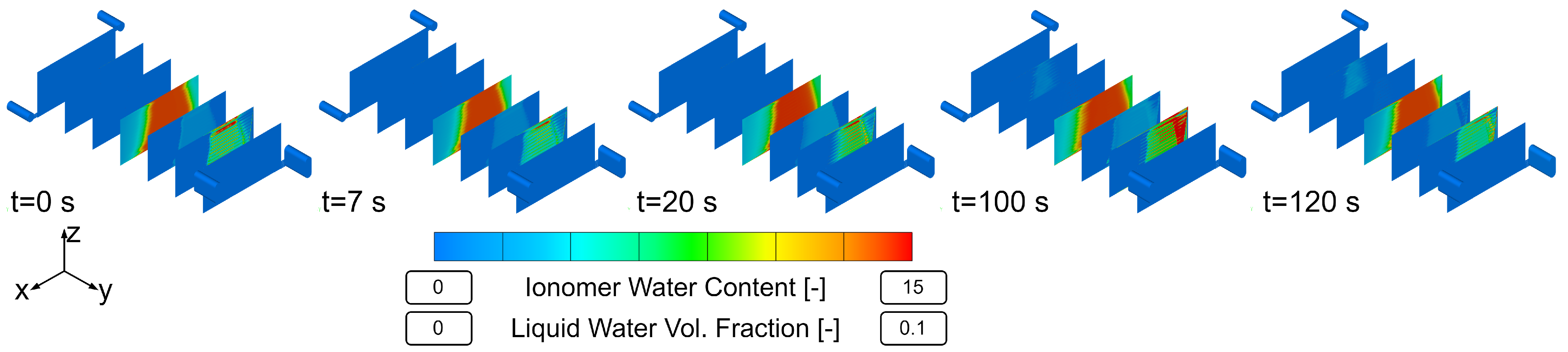
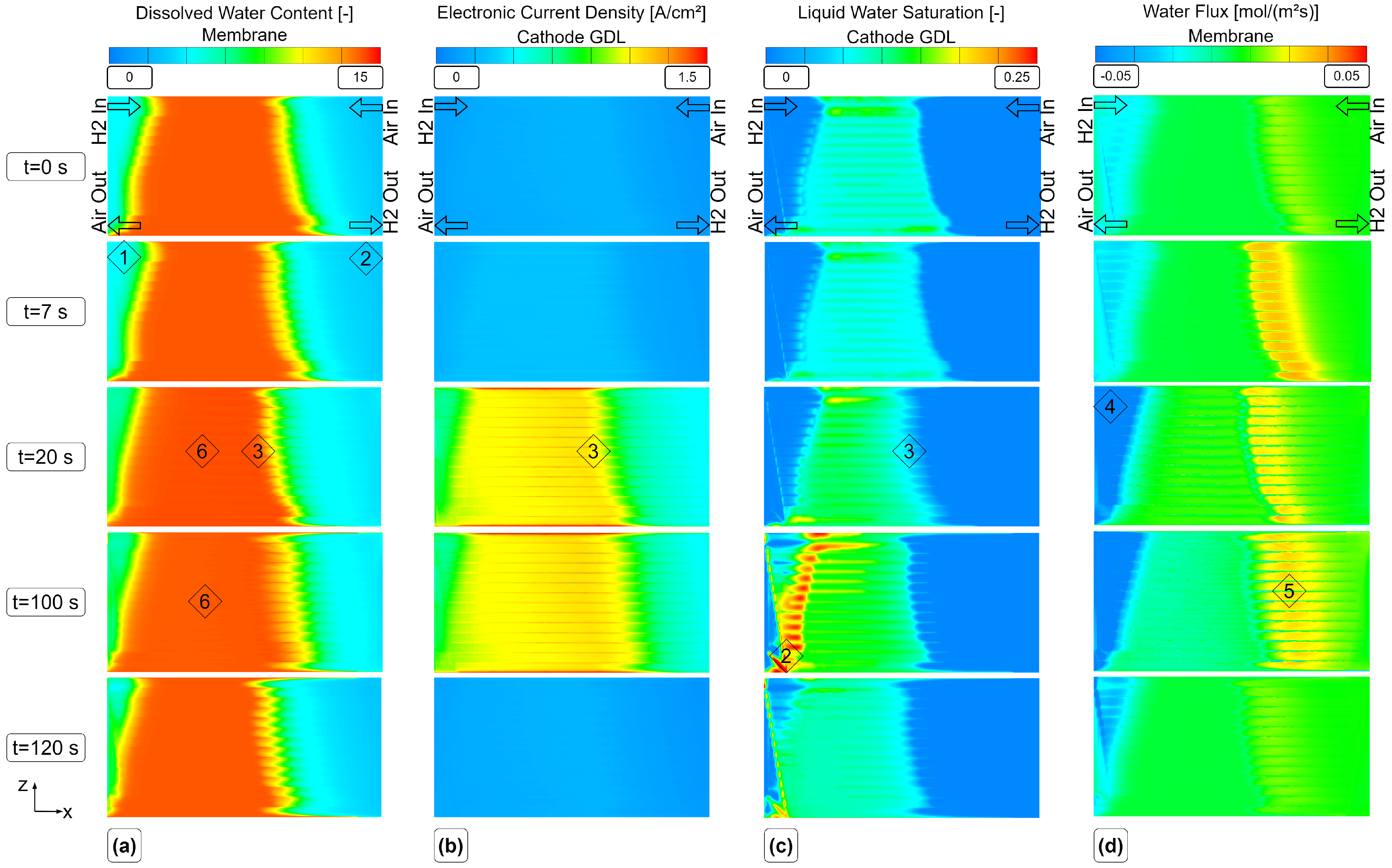
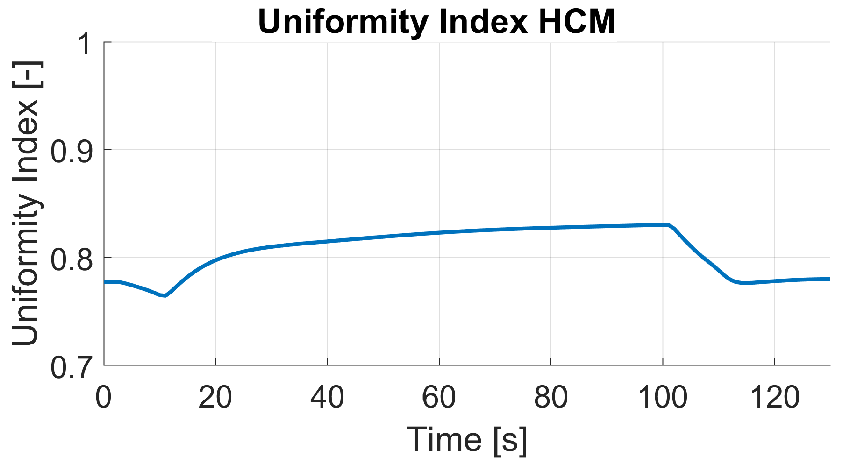
Using this innovative meshing strategy and a suitable parameterization, the transient simulation of a load change was performed and the results are presented. The objective was to show the internal processes and states during transient operation, in particular the effects of liquid water formation and transport on the dissolved water content and electric current uniformity in the cell. Finally, an outlook on further possible investigations on the parameterization of transient CFD models is given.

2. Materials and Methods

2.1. Governing Equations of the 3D-CFD-Model

The 3D-CFD model for low-temperature PEMFCs used in this work is part of the AVL Fire™ M software package. The governing equations of the fuel cell model and the associated source terms and interface conditions can be found in Fink et al. [27]. The model accounts for laminar two-phase flow based on an Euler multi-phase approach with multi-component species diffusion and heat transport in flow channels and porous layers. Electron and ion transport in solid phases, electrochemical reactions in catalyst layers and dissolved water, and species transport in ionomer material are considered. The electrochemical reactions are modeled with the well-known Butler–Volmer equation. Parasitic reactions at opposite electrode due to gas crossover in the membrane are considered. Gas diffusion layers (GDLs) and catalyst layers (CLs) are defined as porous material and are modeled using volume-averaging methods such as the Darcy equation, including capillary effects. Because the mass transport limitations at the cathode were not relevant, the more sophisticated agglomerate model was not used. The macrohomogeneous approach was activated, which further accelerated the simulation and to achieve better compatibility with the quasi-3D model used for the parameterization.

2.2. Geometry of the Investigated Fuel Cell

The investigated fuel cell was part of a 30 $\mathrm{k}$$\mathrm{W}$ PEMFC stack. The bipolar plates were made out of graphite and had imprinted gas channels. Liquid cooling was used to remove excess heat, and the cooling channels were located inside the bipolar plates. GDLs were made from carbon paper with hydrophobic treatment and microporous layer (MPL). The total thickness of the MEA was 450 $\mathsf{\mu }$m in compressed state with 210 $\mathsf{\mu }$$\mathrm{m}$ for each GDL, 10 $\mathsf{\mu }$$\mathrm{m}$ for the CCL, 5 $\mathsf{\mu }$$\mathrm{m}$ for the anode catalyst layer (ACL), and 15 $\mathsf{\mu }$$\mathrm{m}$ for the membrane. Hydrogen and air were in counter-flow setup. The y-direction was the through-plane direction. The cooling inlet was on the side of the air inlet and hydrogen outlet.

2.3. Computational Meshes

The generation of suitable finite-volume meshes for 3D-CFD simulation (preprocessing) is one of the most important tasks in the course of setting up such simulations. The computational time, accuracy, and required computational resources are strongly influenced by the size and quality of the resulting computational meshes. The unique geometry of fuel cells, thin in the main current flow direction but up to two orders of magnitude larger in the other two dimensions, presents a challenge for proper discretization. In particular, the small dimensions of the gas channels and the minimum requirements for capturing all flow phenomena can drive the number of computational cells into regions as large as 100 M. The presented computational meshes were created with the AVL FAME™ M mesher, which is part of the software package used.

Three different meshing approaches are presented in the following sections. The first approach is the most simplified one, as it represents one gas channel of the fuel cell. In this approach, the behavior of the FC is averaged on a gas channel. As a result, the effects of non-symmetry in the in-plane direction (x-z plane) of the MEA are not captured. However, the resulting small number of computational cells keeps the simulation time low.

The most detailed approach is to discretize the whole fuel cell geometry as is. Local effects and processes can be captured with high detail, e.g., the influence of the land area between the channels on the species concentration is visible. The main drawback is the large number of computational cells for fuel cells with large active area.

A reduction of computational cells could be achieved by an innovative approach, the homogenized channels mesh. The imprinted flow field of the bipolar plate was replaced with porous sections and these sections steered the flow, with the help of anisotropic permeabilities, into the direction of the original flow field. This approach is not as detailed as the discretization of the entire FC, e.g., the effects of land areas between channels cannot be captured due to the averaging approach. However, as the results later show, the local distributions are predicted very similarly. The much smaller number of computational cells allows simulation of longer load profiles with moderate computational effort.

The MEA was extruded with 5 layers of each GDL, 6 layers for each CL, and 10 layers for the membrane (five at the anode and five at the cathode side). The MPL was not modeled in order to keep the number of unknown material parameters low.

2.3.1. Single-Channel Model (SCM)

The channel model mesh represents a simplification of the geometry by reducing the original fuel cell geometry to a channel. Compared to the later-presented discretization approaches, this leads to a much smaller cell count and thus faster computation times. Furthermore, the channel model represents the same part of the fuel cell as the quasi-3D model used for parameterization. Due to the serpentine flow field, the channel model is longer than the actual width of the fuel cell. Hexahedral cells were used to discretize the channel geometry. Symmetry conditions were applied to further reduce the number of computational cells (see Figure 1). The terminal boundary faces were also used to apply cooling boundary conditions (BCs). The in/outlet sections of the gas channels were extruded to develop the flow before entering the fuel cell.

Table 1. Number of computational cells of single-channel model approach.

	Cathode	Anode
Bipolar Plate	100,000	114,000
Channels	41,200	57,680
GDL	60,000	55,000
CL	72,000	66,000
Membrane	115,000
Sum	680,880

shows the resulting number of computational cells.

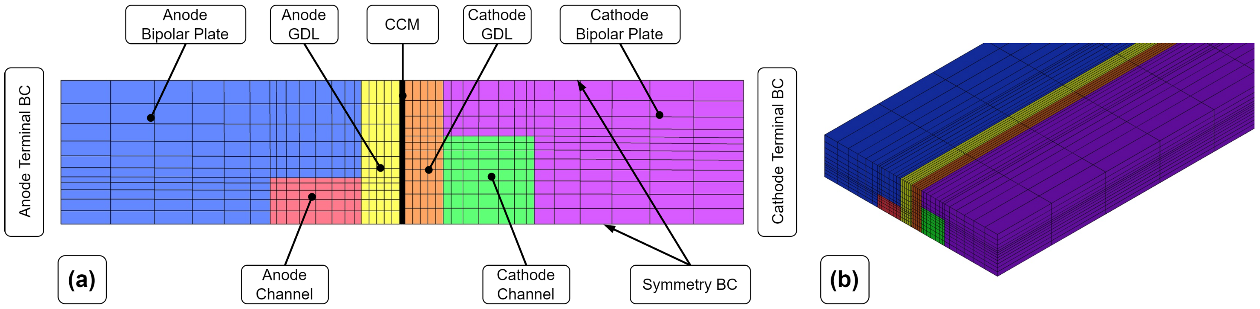
2.3.2. Fully Resolved Channels Model (FRCM)

For the fully resolved mesh, anode and cathode bipolar plate were meshed independently with polyhedral cells. Since anode and cathode flow field design were different, no symmetry could be used. Inside the gas channels, one boundary layer was created to account for the wall treatment. The minimum cell size was chosen to have at least three computational cells (excluding the boundary layer cells) at the height of the gas channels to achieve a compromise between accuracy and computational time. GDL, CL, and the membrane were extruded starting from the created polyhedral mesh. The membrane is divided in the middle into an anode and a cathode part, connected with an arbitrary connection (non-conformal mesh interface) due to non-symmetry of the cell geometry.

The resulting number of generated computational polyhedral cells is shown in

Table 2. Number of generated polyhedral cells.

	Cathode	Anode
Bipolar Plate	7,216,241	7,392,854
Channels	3,033,899	2,051,519
GDL	3,883,300	3,514,660
CL	4,659,960	4,217,592
Membrane	7,397,960
Sum	43,367,985

. In Figure 2a, the created mesh with the labeling of the parts is shown. Figure 2b shows the meshed geometry of the fuel cell with highlighted boundary faces. Since the gas channels were very small compared to the outline of the fuel cell, this resulted in a large number of computational cells. Therefore, high-performance computers with a sufficient number of cores and RAM were required to perform the 3D-CFD simulations in a reasonable amount of time.

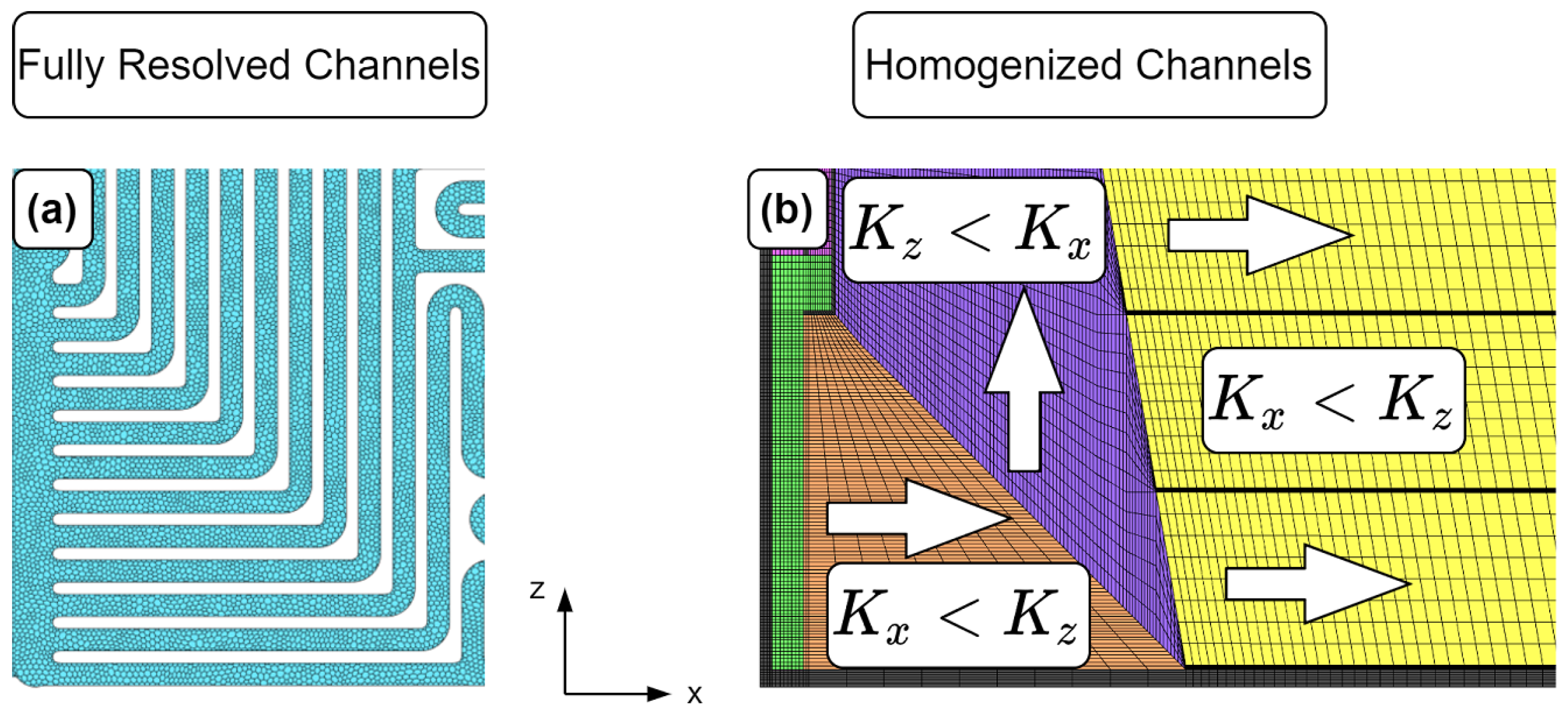
2.3.3. Homogenized Channels Model (HCM)

The computational mesh with fully resolved channels results in a high number of cells, which is not suitable for transient simulations due to high demands of computational power and time. The goal is to significantly reduce the number of computational cells, but maintain the general properties of the flow field. Therefore, the imprinted gas channels were modeled with porous media sections that steer the flow into the original flow direction of the gas channels via anisotropic permeabilities, e.g., if the main direction of the flow field is along the x-axis, the permeability in x-direction is orders of magnitude lower compared to the y- and z-direction. The goal of this approach is to maintain the pressure drop and local distributions of the other variables, as in the FRCM. The application of the porous media approach requires a hexahedral-structured computational mesh of the flow fields. Figure 3 shows the basic principle. The dark sections inside the hexahedral mesh belong to the bipolar plate (=solid region) and were necessary to ensure numerical stability and avoid artificial overshoots of the velocity. Most of the calculated quantities were not visibly affected by the 90° change in direction from one flow steering section to the other. Only the velocity field and liquid water volume fraction show unexpected behavior in the corners of the turns where the skewness and growth ratios of the computational cells are high, but that does not have any big influence on the overall solution. Isotropic permeabilities are defined in the input region (green) to ensure that the flow is not forced to flow in a particular direction.

The hexahedral-structured mesh is embedded into the mesh with polyhedral cells of the bipolar plate and connected with non-conformal mesh interfaces. Based on the isometric views of the created meshes, no difference between the HCM and the FRCM can be seen (see Figure 2b).

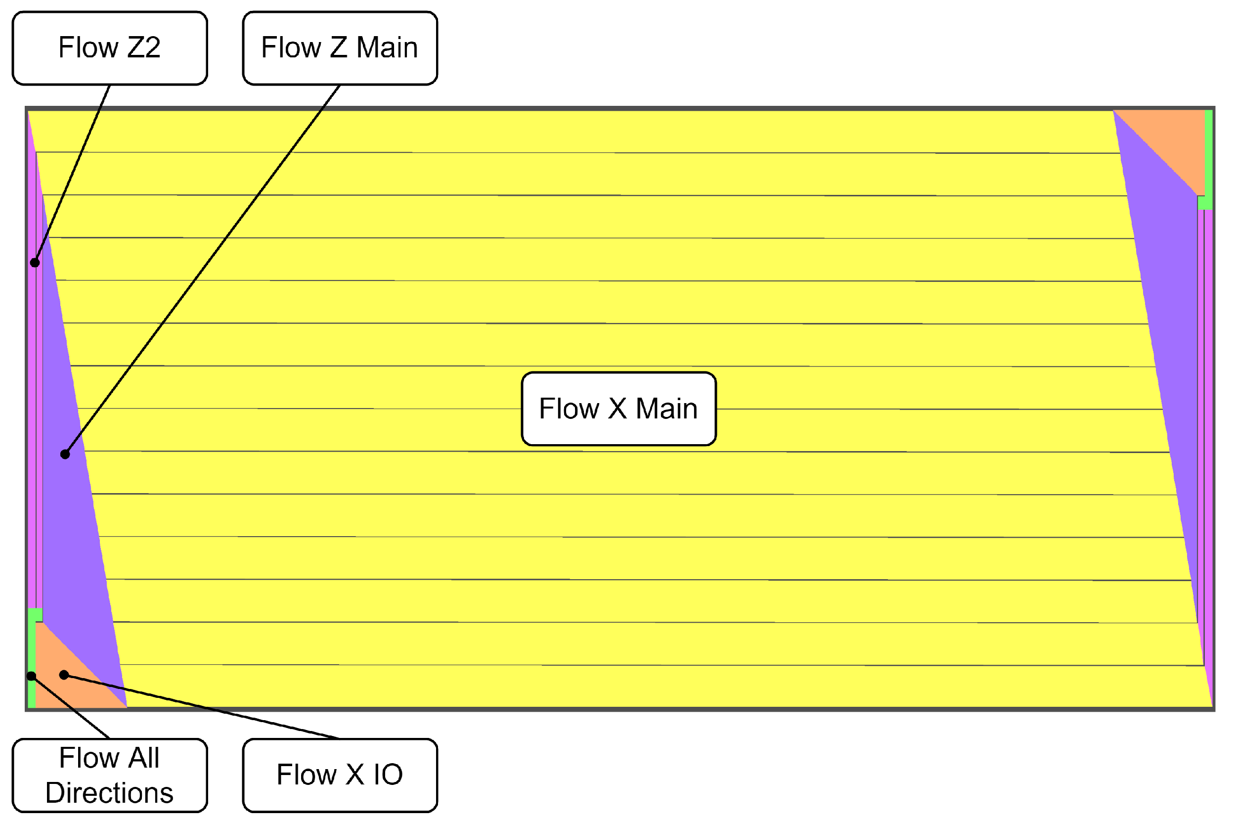
The number of generated computational cells of the homogenized channel mesh is shown in Table 3. The homogenized channel approach reduced the mesh count by a factor of eight compared to the FRCM (see Table 4). The porosity of the gas channels was defined as the ratio between the area where the gas channels have contact with the GDL and the active area. The permeability K in the main flow direction of the respective flow section was calculated based on Darcy’s law [56] in 1D:

$$\frac{\mathrm{d}P}{\mathrm{d}x}=-\frac{\mu }{K}v\Rightarrow K=v\mu \frac{\Delta l}{\Delta P}$$

(1)

where v is the average velocity in the channel, $\mu$ is the dynamic viscosity, $\Delta l$ is the length of the flow steering section, and $\Delta P$ is the pressure drop of the considered flow section. The values for the velocity v and pressure drop $\Delta P$ over the length $\Delta l$ were extracted from a simulation with the fully resolved channels model. The design of the analyzed flow field required the definition of five flow steering sections: (1) Flow All Directions, (2) Flow X IO, (3) Flow Z Main, (4) Flow Z2, and (5) Flow X Main (see Figure 4).

In the through-plane direction (y-direction), the permeability $K_y$ was set to a lower value to avoid too-high species concentration gradients over the depth of the channels.

Table 3. Number of computational cells of homogenized channel approach.

	Cathode	Anode
Bipolar Plate	1,158,408	1,301,646
Channels	474,327	286,403
GDL	377,240	377,240
CL	452,688	452,688
Membrane	754,480
Sum	5,632,120

Table 3. Number of computational cells of homogenized channel approach.

	Cathode	Anode
Bipolar Plate	1,158,408	1,301,646
Channels	474,327	286,403
GDL	377,240	377,240
CL	452,688	452,688
Membrane	754,480
Sum	5,632,120

A comparison of the resulting cell count of the created computational meshes can be found in Table 4.

Table 4. Comparison of total number of computational cells of the resulting models.

	Number of Cells	Reduction
Fully Resolved Channels Model (FRCM)	43,367,985
Homogenized Channels Model (HCM)	5,632,120	−87% to FRCM
Single-Channel Model (SCM)	680,880	−88% to HCM

Table 4. Comparison of total number of computational cells of the resulting models.

	Number of Cells	Reduction
Fully Resolved Channels Model (FRCM)	43,367,985
Homogenized Channels Model (HCM)	5,632,120	−87% to FRCM
Single-Channel Model (SCM)	680,880	−88% to HCM

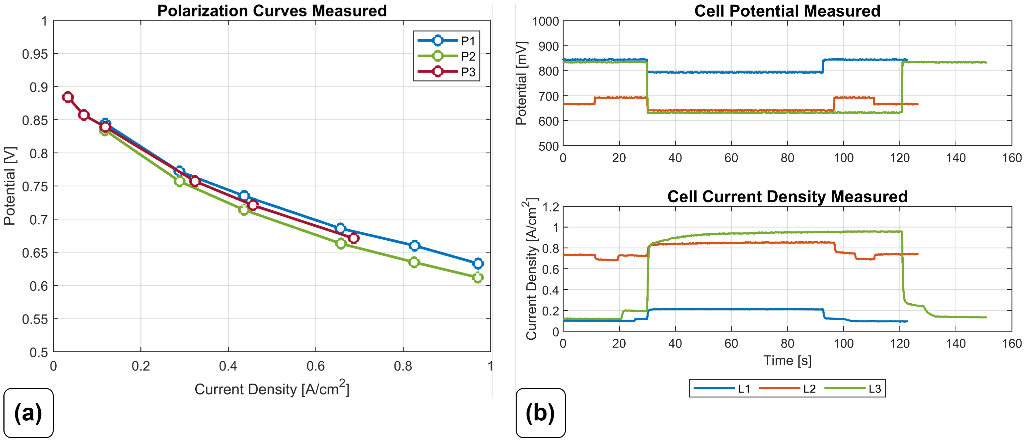
2.4. Experimental Data

The used experimental data are described in detail in Haslinger et al. [55]. Three polarization curve measurements at different anode inlet pressures and cooling temperatures, as well as three load steps with approximately 120 $\mathrm{s}$ duration, were available for simulation and validation. Figure 5 shows the measured curves.

2.5. Numerical Settings

The numerical settings can influence a CFD simulation significantly and have to be customized for every simulation. In this paper, results from steady-state and transient simulations are presented. The maximum steady-state iterations for the FRCM and HCM were set to 7500 to obtain a converged solution. The initialization of the transient simulations was performed with quasi-steady-state time steps to have a converged solution as initial condition for the transient time stepping. The time step sizes were set according to the gradients of voltage, current density, and air mass flow and varied from 50 ms (high gradients) to 200 ms (low gradients). The iterations per time step ranged from 20 for SCM to 50 for HCM. With that approach, sufficient low residuals were achieved.

2.6. Boundary Conditions

In

Table 5. Boundary conditions for presented numerical models.

Face	Mass Flow	Temp.	Pressure	Mole Fraction	Thermal	Electric
Anode Inlet	${\dot{m}}_{ano,in}$	${\vartheta }_{ano,in}$		H2/H2O 1/$\phi =0.99$
Anode Outlet			$p_{ano,out}$
Anode Terminal					0 W/m${}^2$	fixed with 0 V
Anode Cooling		${\vartheta }_{ano,cool}$			$HTC=1831$ W/(m${}^2$K)
Cathode Inlet	${\dot{m}}_{cat,in}$	38 °C		O2/N2/H2O 0.21/0.79/$\phi =0.3$
Cathode Outlet			$p_{cat,out}$
Cathode Terminal					0 W/m${}^2$	$U_{cell}$/$i_{cell}$
Cathode Cooling *		${\vartheta }_{cat,cool}$			$HTC=1831$ W/(m${}^2$K)

* For SCM, cooling and terminal boundary faces coincide.

, the boundary conditions are listed. The electric potential at the anode terminal surfaces was 0 $\mathrm{V}$ and $U_{cell}$ at the cathode side for voltage-driven simulations (load steps). For the simulation of the polarization curves, the current density was prescribed at the cathode terminal faces. Excess heat was removed by heat convection, and a heat transfer coefficient and average cooling temperature were specified at the cooling faces. The remaining boundary faces were of the wall type, with no heat flux and a current density of zero. In the SCM, the electrical connection and cooling surfaces coincide. In addition, the SCM model had symmetric boundary conditions to reduce the number of computational cells.

2.7. Model Parameterization

A transient, single-phase, non-isothermal, quasi-3D model of a PEMFC based on the previous work of the authors [55] was used to conduct the numerical optimization of parameters. The identification of the parameters with the greatest influence on performance was based on the results of Karpenko-Jereb et al. [28]. They used the same CFD code as in this work to perform a theoretical study of the influence of parameters on the performance of a PEMFC. Their result is consistent with other sensitivity analyses of fuel cell models found in the literature [18,57].

It turned out that some of the parameters obtained from the numerical optimization process need further adjustments when used with the CFD models to predict the measured current density and potential accurately. The reasons for the discrepancies were, first, a different membrane water model, and, second, that the quasi-3D model did not account for the ohmic losses in the CLs [58]. Low simulation times of the SCM allowed fast parameter variations with that model due to the reduced cell count compared to the FRCM and HCM. The following methodology was developed to achieve the best agreement with the measured data:

• Quasi-3D Model:
  Perform numerical optimization of parameters with a high number of function evaluations and measurement data as reference.
• Transfer to CFD:
  The reference ionic conductivity from the numerical optimization with the quasi-3D model had to be multiplied by 3. This was necessary in order to account for the ionic losses in membrane, ACL, and CCL because the used quasi-3D model did not account for ionic losses in the CLs. The factor of 3 was derived from the thicknesses of the parts and the assumption that the proton concentration in- and decreases with a constant gradient in the CLs. When ultra-thin membranes are used, the ion losses of the CLs may exceed the ion losses in the membrane. Therefore, modeling of the ion losses in the CLs is required to account for the actual ohmic losses. The SCM, as the simplest and fastest of the CFD models, was used to obtain a first glance at how the derived parameters behave with the CFD model. It turned out that some minor adjustments to the reference exchange current density and ionic conductivity were necessary to obtain a better agreement of the results of the CFD models with the measured data.
• HCM/FRCM:
  Use the updated parameter set to simulate more sophisticated models such as the FRCM or HCM.

For the optimization, only load step L3 was used as a reference; the other measured curves were used for validation purposes of the results.

3. Results and Discussion

3.1. Parameterization Results with Quasi-3D Model and SCM

The following parameters were used as design variables for the numerical optimization of parameters: (1) reference exchange current density $i_{0,ref}$, (2) electron transfer coefficient $\alpha$, (3) activation energy of RECD $E_{act,i_0,ref}$, (4) reference ionic conductivity ${\sigma }_{ion,ref}$, (5) dissolved diffusion water coefficient $D_{w,ref}$, (6) electronic conductivity of GDL ${\sigma }_{elec,GDL}$, (7) porosity of GDL ${\epsilon }_{GDL}$, and (8) tortuosity of GDL ${\tau }_{GDL}$. The other constant (material) parameters can be found in Appendix A.

The obtained parameter values of the numerical optimization with the respective bounds of the design variables are shown in

Table 6. Numerical optimization results with quasi-3D model (DVS8 L3) and final parameter set of SCM and HCM (DVS8 CFD) are shown. The differences between the two sets are in $i_{0,ref}$ and ${\sigma }_{ion,ref}$.

Parameter	${\mathit{i}}_{0,\mathbf{ref}}$	${\mathit{E}}_{\mathbf{act},{\mathit{i}}_0,\mathbf{ref}}$	$\mathit{\alpha }$	${\mathit{\sigma }}_{\mathbf{ion},\mathbf{ref}}$	${\mathit{D}}_{\mathit{w},\mathbf{ref}}$	${\mathit{\sigma }}_{\mathbf{elec},\mathbf{GDL}}$	${\mathit{\epsilon }}_{\mathbf{GDL}}$	${\mathit{\tau }}_{\mathbf{GDL}}$	$\mathit{\epsilon }/\mathit{\tau }$
Unit	A/m3	J/mol	-	S/m	m2/s	S/m	-	-	-
Bound min	1.00 × 105	50,000	0.25	0.2	5 × 10−12	125	0.4	1	-
Bound max	1.00 × 106	100,000	0.5	2	5 × 10−10	350	0.8	4	-
DVS8 L3	6.63 × 105	58,237	0.33	0.72	6.7 × 10−11	350	0.79	1.3	0.61
DVS8 CFD	1.02 × 106	58,237	0.33	2.28	6.7 × 10−11	350	0.79	1.3	0.61

. The bounds are based on known physical values from the literature [47].

The obtained low reference ionic conductivity at a reference water content of 14 (fully hydrated) and a reference temperature of 25 °C is noteworthy. Based on the membrane data sheet, an ionic conductivity of 14 S/m would be expected for a fully hydrated membrane. However, only with this small value was the shape of the current density of load step L3 simulated correctly.

3.2. Simulation Results of Load Steps and Polarization Curves with Quasi-3D Model and SCM

The simulations with the parameters obtained from the parameterization procedure not only showed good agreement with the reference load step L3 but also with other available measurement data. In addition, steady simulations of the polarization curves were conducted. The simulation of the quasi-3D model of one load step took approximately 60 s (real time factor 0.5) on an Intel Xeon E5-1620v3 CPU. The SCM was simulated on the Vienna Scientific Cluster 4 (VSC 4) and the simulation of L3 needed 6.5 h on 48 cores. Whereas the quasi-3D model has only a transient option, the CFD models can be set up as steady or unsteady simulation. This means that for polarization curve simulations with the quasi-3D model, the load had to be applied rather slowly to achieve quasi-stationary states.

The simulation results in Figure 6 show very good agreement with measured data. Although the parameters were fitted with L3 only as a reference and the models differ significantly mathematically (quasi-3D model with real-time capability versus 3D-CFD model), the results of both models predicted the voltage/current behavior of the fuel cell under study with similar accuracy. Results from the polarization curve P2 simulated with the HCM were added as well, and showed minor deviation to the experimental data. Although only L3 was used as a reference for numerical optimization of the parameters, the simulation results of the polarization curves also showed very good agreement with the measured data. More detailed results of the quasi-3D and SCM are shown and discussed in Section 3.4.

3.3. Comparison of Fully Resolved Channels Model and Homogenized Channels Model

Figure 7 shows the simulated pressure drop between the channel inlet and outlet for different loads. The values were normalized to the inlet pressures of anode and cathode, respectively. The pressure drops in the cathode channels were nearly the same with both meshes, whereas the pressure drops in the anode channels differed slightly at higher current densities (=higher species mass flows).

Not only is the pressure distribution in the channels important, so too is the distributions of, e.g., the membrane water content, electrical current density, or liquid water accumulation. Figure 8 shows a selection of quantities of interest. The anode inlet is at the left upper side and the anode outlet is at the right lower side, whereas the cathode inlet is at the right upper side and the cathode outlet at the left lower side. The local distribution of the quantities agreed well between the two models, so that the HCM had similar abilities to predict the internal states as the more sophisticated FRCM.

In Figure 8, the characteristics of the homogenized channels mesh can be seen. The solid sections between the channel sections are visible and produce higher values of, e.g., dissolved water content in the MEA, although they are very thin. The liquid water saturation in the middle of the cathode GDL showed numerical issues. Here, artificially high values at the 90° turns can be observed, but this seems to have no visible influence on the other solution quantities of interest. Although the local saturation with liquid water in the cathode GDL differs in absolute values, the position where liquid water forms agrees well between the models.

3.4. Transient 3D-CFD Simulation of Load Step L3

The simulated models were parameterized with the parameters obtained from the calibration procedure (see Table 6). The missing parameters can be found in Appendix A. With these parameters, the simulations predicted the measured current density and voltage with high accuracy. In the following, the simulation results of load step L3 are shown. The transient 3D-CFD simulation of 130 s with the HCM required 9 days and 18 h with 48 cores at the Vienna Scientific Cluster 4.

Figure 9 shows the simulation results and the model differences between quasi-3D and CFD models. Since the load step was voltage-driven at the test bench, the typical undershoot of voltage [38] was not seen with these results, but the current density needed approximately 60 s to reach a steady state. Not only the shape of the current density, but also the absolute values were predicted well with all models.

The membrane water content and the activation overpotential in the CCL were predicted differently. The overpotential in the CCL was higher with the quasi-3D model and had a different shape. The reason for this is that the quasi-3D model did not consider liquid water (one-phase model); hence, the local partial pressure of water vapor was higher and affected the exchange current density and the ionomer water content directly. Furthermore, the CFD model considered additional water transfer resistances from the fluid phase to the dissolved phase in the ionomer; therefore, the ionomer water content was predicted higher with the quasi-3D model. The shape of the current density is directly influenced by the activation and ohmic overpotential via the Butler–Volmer equation. Thus, the exchange current density and ionomer water content had a significant effect on the result. The exchange current density itself depends strongly on the course of the oxygen and water vapor concentration and the temperature of the CCL. In turn, the oxygen concentration depends on the diffusion processes in CL and GDL. Summed up, the simulated course of the current is obtained.

No results of the liquid water volume fractions, as well as dissolved water flow, in the membrane were available from the quasi-3D model. With the CFD models, the water buildup and transport can be investigated. The volume fractions of the liquid water in anode GDL and cathode CL are shown. During the simulated load step, low liquid water accumulation in the porous parts can be observed. The SCM predicts more liquid water in the anode GDL during the load change. This is an indication that the actual liquid water distribution of large active area fuel cells is not predicted well with simplified models such as the SCM. The effects of the additional extension of the active area in the z-direction must not be underestimated. Additionally, the removal of liquid water after the load change back to low load was faster with the SCM than compared to the HCM.

Electroosmotic drag and diffusion of water were used by the CFD models to simulate the dissolved water flux in the membrane. It shows that after the load change to high values (10 s $<t<100$ s), the diffusion of water from the cathode to the anode dominates (negative values indicate water flow from cathode to anode, and positive values—vice versa). This is in contrast to the observations made by [44], where an anode dryout was mentioned when high currents were drawn from the fuel cell; however, they used a different relationship between the diffusion coefficient and the water content, and their used membrane was more than three times thicker.

Figure 9 shows the good agreement of the two CFD models, although the SCM is significantly simpler than the HCM. The SCM represents only one channel of the total fuel cell geometry, thus the distributions in the x-z plane could not be well calculated. However, the internal states were predicted very similarly, but the membrane water content and liquid water saturation seem to depend on the actual distribution over the whole active area (in x-z plane). The symmetry of the internal distributions of the fuel cell studied was not present in either the z or x directions. Therefore, the SCM can only predict an average state inside the MEA. Although the SCM was quite coarse-meshed to keep the simulation time low, the agreement between the SCM and HCM results was very high. In the following, the results of the more sophisticated HCM are shown.

The 3D plots in Figure 10 and Figure 11 represent states at the beginning $t=0$ s and end $t=120$ s of the simulated time. In addition, one time before the main load step, $t=7$ s, where the air mass flow was increased, two times shortly after the main load step, $t=20$ s, and at the end of the main load step, $t=100$ s, are shown.

In Figure 10, an exploded view of the fuel cell shows the liquid water accumulation of the fuel cell parts at different times. The liquid water volume fraction is shown in all parts except the membrane, where the ionomer water content is shown. It can be observed that almost no liquid water was present in the anode side of the fuel cell. After 100 s, a small amount of liquid water is visible in the anode GDL, which increased after the load changed back to low currents ($t>100$ s).

Figure 11 shows a selection of 3D results of the quantities to be discussed. The highest values of all the distributions were shifted to the left (negative x-direction). Due to the dry supply air, the dissolved water content in the membrane near the cathode inlet was particularly low, with a trapezoidal shape of the maximum values (see Figure 11a). The reason for the trapezoidal shape is that the inlets and outlets of fuel and oxidant were not directly opposite, but crossed. A slight increase of the maximum values of the dissolved water content towards the species inlets between $t=$ 20 s and $t=$100 s can be observed (Marker 6). The incoming air (Marker 2) and hydrogen (Marker 1) have a lower temperature compared to the fuel cell; hence, they were heated up and wanted to humidify itself with the produced water by the electrochemical reaction. Therefore, the water was not available for increasing the dissolved water content in the ionomer. The humidification strategy of counter-flow setups is that the humidified gas of the cathode humidifies the incoming gas of the anode and vice versa. The membrane has to shift the water from one electrode to the other, which is illustrated in Figure 11d with the dissolved water flux in the membrane. Marker 4 shows that near the hydrogen inlet, dissolved water flows from cathode to anode (negative values), and Marker 5 shows the opposite: dissolved water flows from anode to cathode (positive values). Between these markers, where dissolved water content in the membrane and liquid water saturation in the cathode GDL were also high, the dissolved membrane water flux was almost 0. When the cell voltage was lowered and the current density increased, $20\mathrm{s}<t<100\mathrm{s}$, the distribution of current was not uniform (see Figure 11b). The highest values of current density (=highest electrochemical reaction rate) occurred where the membrane had the highest dissolved water content values (=low ionic resistance) and no liquid water hinders the oxygen from flowing to the reaction sites (=low diffusion losses) (see Marker 3). This had a direct effect on the ionic conductivity of the membrane and resulted in higher values and thus lower protonic resistance. Similar observations were made in [27,38].

As mentioned above, the solid sections in the flow field influenced maximum values of the variables. The saturation with liquid water had the highest values in this area, as can be seen in Figure 11c. The reason for this is that the gas velocity in the channels was low at these locations and therefore the removal of liquid water was not as efficient as in the fully developed flow. Furthermore, liquid water was formed, where the membrane water content had its highest values and could not uptake more water. Near the cathode inlet, no liquid water was present, because the water was needed to humidify the incoming air.

It is important to avoid starvation of the fuel or oxidizer due to flooding of the pores in the GDL and CL, and dehydration of the ionomer to prevent degradation [59]. A high water content of the ionomer means that the ionomer no longer has water adsorption potential, but the water generated by the electrochemical reaction must be removed. When the ionomer is fully saturated, liquid water forms in the pores of GDL and CL or gas channels and can clog them, leading to fuel or oxidizer starvation. Since liquid water saturation did not exceed a local value of 0.25 in the cathode GDL (25% of the void volume is filled with liquid), clogging of the pores did not pose a concern.

Figure 11 shows that the current density is highest where the membrane has the highest value of dissolved water. Thus, a uniform distribution of water content can improve fuel cell performance by allowing more current to be drawn. This could be achieved by external humidification of hydrogen and air to increase the relative humidity of the gases at the inlets. The uniformity index (UI) indicates how evenly a quantity is distributed over an area. In this work, the uniformity index of the dissolved water content in the membrane was calculated based on the results of the HCM (see Figure 12). It can be observed that the UI slightly increased until the end of the load step (10 s $<t<100$ s) and had a maximum value of 0.83.

4. Conclusions

The parameterization and the vast amount of resulting computational cells of 3D-CFD models of large active area FCs are challenging. In this work, both issues were addressed. The optimal parameter set was obtained using a quasi-3D model and numerical optimization methods with experimental data as a reference. A set of eight parameters (design variables), characterizing different parts of the polarization curve, were selected. Experimental data for calibration and validation from a stack test bench were available. Three measured polarizaton curves with different anode inlet pressures and cooling temperatures, as well as three load steps in different current regions, were recorded at the test bench. The load step with the biggest change in load was used as a reference for numerical optimization of parameters.

For the 3D-CFD simulations, three different meshing approaches with different levels of detail were presented: the SCM, FRCM, and HCM. As a first step, the SCM was parameterized with the obtained parameter set by the numerical optimization procedure. With minor adjustments to the reference exchange current density and the reference ionic conductivity, very good agreement between simulated and measured load steps and polarization curves was obtained. The use of only one load step that covers the full range of possible fuel cell current is enough to obtain a set of parameters that are able to simulate not only dynamic load changes but also steady-state polarization curves with high accuracy.

The SCM has only minor capabilities of representing the actual distribution of quantities over the active area. Thus, more detailed 3D-CFD models were created. The FRCM resulted in about 43 M computational cells, which might be used for steady-state simulations but not applicable for unsteady simulations of up to several minutes of physical time. To enable transient 3D-CFD simulations of the entire geometry of the fuel cell and simulate more than a few seconds in a reasonable computation time, an alternative meshing approach, the homogenized channel model, had to be used. With that approach, it was possible to reduce the cell count by about 87%, enabling the unsteady simulation of a load step with the high temporal and spatial distribution. The final parameter set obtained and improved with the SCM was used for parameterization of the HCM.

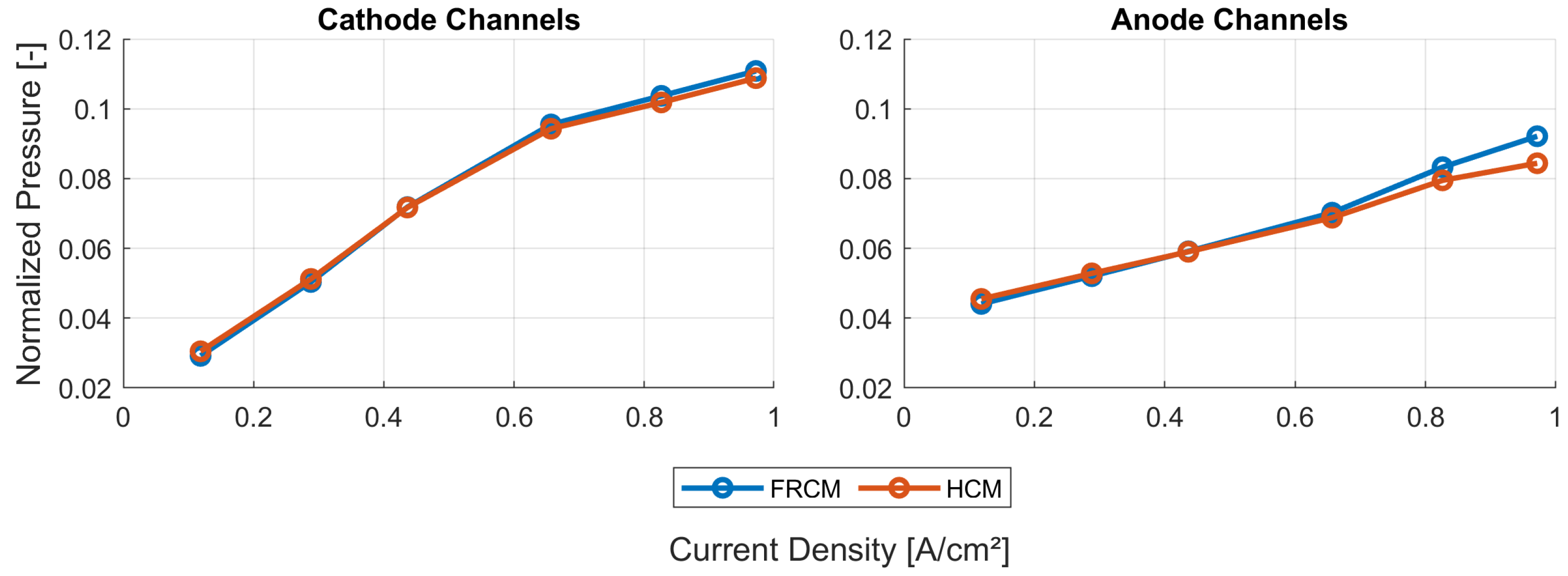
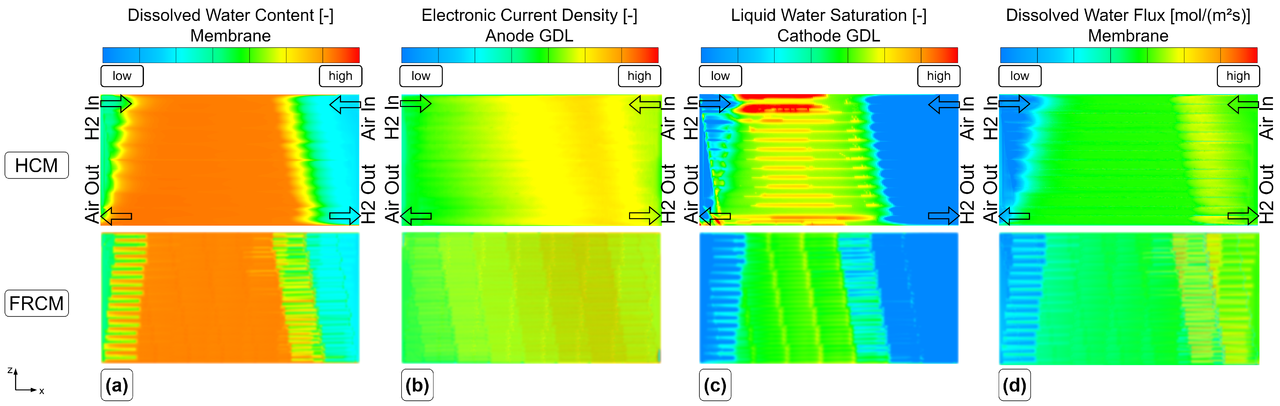
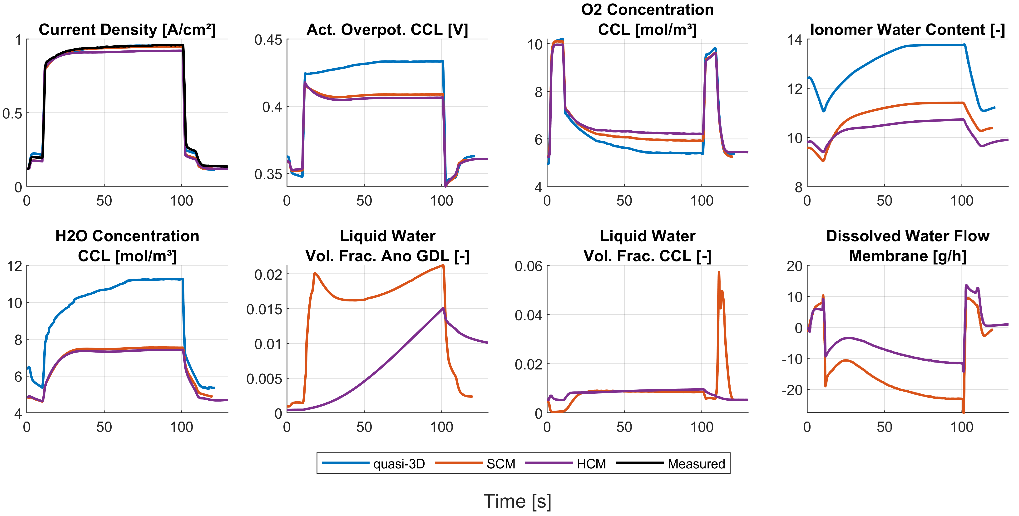
The steady-state results between the fully resolved and homogenized channel approach revealed only minor differences in pressure drop and distributions of solution quantities. One of the three available load steps (L3) from experimental data was simulated with the HCM, and the simulation results showed an excellent agreement of voltage and current with the measured data. Further insights into the processes and especially the connection of water management and current density during a steep load step of a PEMFC were made visible and discussed. Possible future work may include the reduction of design variables for the numerical optimization process. In addition, the authors experienced uniqueness problems with the obtained parameter set, as discussed in [60]. Therefore, more detailed measurements need to be performed on the materials used in order to obtain a parameterization of the fuel cell model that reflects the actual material parameters as well as possible.

References

1. Barbir, F. PEM Fuel Cells: Theory and Practice, 2nd ed.; Elsevier: Amsterdam, The Netherlands; Academic Press: Boston, MA, USA, 2013. [Google Scholar]
2. Mitsushima, S.; Hacker, V. Role of hydrogen energy carriers. In Fuel Cells and Hydrogen; Elsevier: Amsterdam, The Netherlands, 2018; pp. 243–255. [Google Scholar] [CrossRef]
3. Nguyen, H.L.; Han, J.; Nguyen, X.L.; Yu, S.; Goo, Y.M.; Le, D.D. Review of the Durability of Polymer Electrolyte Membrane Fuel Cell in Long-Term Operation: Main Influencing Parameters and Testing Protocols. Energies 2021, 14, 4048. [Google Scholar] [CrossRef]
4. Bethoux, O. Hydrogen Fuel Cell Road Vehicles: State of the Art and Perspectives. Energies 2020, 13, 5843. [Google Scholar] [CrossRef]
5. Klell, M.; Eichlseder, H.; Trattner, A. Wasserstoff in der Fahrzeugtechnik; Springer Fachmedien Wiesbaden: Wiesbaden, Germany, 2018. [Google Scholar] [CrossRef]
6. O’Hayre, R.P.; Prinz, F.B.; Cha, S.W.; Colella, W.G. Fuel Cell Fundamentals, 3rd ed.; Wiley: Hoboken, NJ, USA, 2016. [Google Scholar] [CrossRef]
7. Zhao, J.; Li, X. A review of polymer electrolyte membrane fuel cell durability for vehicular applications: Degradation modes and experimental techniques. Energy Convers. Manag. 2019, 199, 112022. [Google Scholar] [CrossRef]
8. Karpenko-Jereb, L.; Araki, T. Modeling of polymer electrolyte fuel cells. In Fuel Cells and Hydrogen; Elsevier: Amsterdam, The Netherlands, 2018; pp. 41–62. [Google Scholar] [CrossRef]
9. Deng, X.; Zhang, J.; Fan, Z.; Tan, W.; Yang, G.; Wang, W.; Zhou, W.; Shao, Z. Understanding and Engineering of Multiphase Transport Processes in Membrane Electrode Assembly of Proton-Exchange Membrane Fuel Cells with a Focus on the Cathode Catalyst Layer: A Review. Energy Fuels 2020, 34, 9175–9188. [Google Scholar] [CrossRef]
10. Springer, T.E. Polymer Electrolyte Fuel Cell Model. J. Electrochem. Soc. 1991, 138, 2334. [Google Scholar] [CrossRef]
11. Bernardi, D.M.; Verbrugge, M.W. A Mathematical Model of the Solid-Polymer-Electrolyte Fuel Cell. J. Electrochem. Soc. 1992, 139, 2477. [Google Scholar] [CrossRef]
12. Cheddie, D.; Munroe, N. Review and comparison of approaches to proton exchange membrane fuel cell modeling. J. Power Sources 2005, 147, 72–84. [Google Scholar] [CrossRef]
13. Demuren, A.; Edwards, R.L. Modeling proton exchange membrane fuel cells—A review. In 50 Years of CFD in Engineering Sciences; Springer: Singapore, 2020; pp. 513–547. [Google Scholar] [CrossRef]
14. Zhao, J.; Li, X.; Shum, C.; McPhee, J. A Review of physics-based and data-driven models for real-time control of polymer electrolyte membrane fuel cells. Energy AI 2021, 6, 100114. [Google Scholar] [CrossRef]
15. Murschenhofer, D.; Kuzdas, D.; Braun, S.; Jakubek, S. A real-time capable quasi-2D proton exchange membrane fuel cell model. Energy Convers. Manag. 2018, 162, 159–175. [Google Scholar] [CrossRef]
16. Ritzberger, D.; Hametner, C.; Jakubek, S. A Real-Time Dynamic Fuel Cell System Simulation for Model-Based Diagnostics and Control: Validation on Real Driving Data. Energies 2020, 13, 3148. [Google Scholar] [CrossRef]
17. Tavčar, G.; Katrašnik, T. A computationally efficient hybrid 3D analytic-numerical approach for modelling species transport in a proton exchange membrane fuel cell. J. Power Sources 2013, 236, 321–340. [Google Scholar] [CrossRef]
18. Goshtasbi, A.; Chen, J.; Waldecker, J.R.; Hirano, S.; Ersal, T. Effective Parameterization of PEM Fuel Cell Models—Part I: Sensitivity Analysis and Parameter Identifiability. J. Electrochem. Soc. 2020, 167, 044504. [Google Scholar] [CrossRef]
19. Kone, J.P.; Zhang, X.; Yan, Y.; Hu, G.; Ahmadi, G. CFD modeling and simulation of PEM fuel cell using OpenFOAM. Energy Procedia 2018, 145, 64–69. [Google Scholar] [CrossRef]
20. Hontañón, E.; Escudero, M.J.; Bautista, C.; Garcia-Ybarra, P.L.; Daza, L. Optimisation of flow-field in polymer electrolyte membrane fuel cells using computational fluid dynamics techniques. J. Power Sources 2000, 86, 363–368. [Google Scholar] [CrossRef]
21. Iranzo, A.; Muñoz, M.; Rosa, F.; Pino, J. Numerical model for the performance prediction of a PEM fuel cell. Model results and experimental validation. Int. J. Hydrog. Energy 2010, 35, 11533–11550. [Google Scholar] [CrossRef]
22. Ferreira, R.B. Two-Phase Flow in PEM Fuel Cells: 1D + 3D Model Development and Numerical Simulations. Ph.D. Thesis, University of Porto, Porto, Portugal, 2017. [Google Scholar]
23. Berning, T.; Djilali, N. A 3D, Multiphase, Multicomponent Model of the Cathode and Anode of a PEM Fuel Cell. J. Electrochem. Soc. 2003, 150, A1589. [Google Scholar] [CrossRef]
24. Riccardi, M.; d’Adamo, A.; Vaini, A.; Romagnoli, M.; Borghi, M.; Fontanesi, S. Experimental Validation of a 3D-CFD Model of a PEM Fuel Cell. E3S Web Conf. 2020, 197, 05004. [Google Scholar] [CrossRef]
25. Corda, G.; Fontanesi, S.; d’Adamo, A. Methodology for PEMFC CFD Simulation Including the Effect of Porous Parts Compression. Int. J. Hydrog. Energy 2022, 47, 14658–14673. [Google Scholar] [CrossRef]
26. Fink, C. Modelling and Simulation of Multiphase Transport Phenomena in Porous Media with Application to PEM Fuel Cells. Ph.D. Thesis, Graz University of Technology, Graz, Austria, 2009. [Google Scholar]
27. Fink, C.; Gößling, S.; Karpenko-Jereb, L.; Urthaler, P. CFD Simulation of an Industrial PEM Fuel Cell with Local Degradation Effects. Fuel Cells 2020, 20, 431–452. [Google Scholar] [CrossRef]
28. Karpenko-Jereb, L.; Sternig, C.; Fink, C.; Hacker, V.; Theiler, A.; Tatschl, R. Theoretical study of the influence of material parameters on the performance of a polymer electrolyte fuel cell. J. Power Sources 2015, 297, 329–343. [Google Scholar] [CrossRef]
29. Bednarek, T.; Tsotridis, G. Issues associated with modelling of proton exchange membrane fuel cell by computational fluid dynamics. J. Power Sources 2017, 343, 550–563. [Google Scholar] [CrossRef]
30. Zhang, G.; Fan, L.; Sun, J.; Jiao, K. A 3D model of PEMFC considering detailed multiphase flow and anisotropic transport properties. Int. J. Heat Mass Transf. 2017, 115, 714–724. [Google Scholar] [CrossRef]
31. Peng, Y.; Mahyari, H.M.; Moshfegh, A.; Javadzadegan, A.; Toghraie, D.; Shams, M.; Rostami, S. A transient heat and mass transfer CFD simulation for proton exchange membrane fuel cells (PEMFC) with a dead-ended anode channel. Int. Commun. Heat Mass Transf. 2020, 115, 104638. [Google Scholar] [CrossRef]
32. Chen, X.; Yu, Z.; Yang, C.; Chen, Y.; Jin, C.; Ding, Y.; Li, W.; Wan, Z. Performance investigation on a novel 3D wave flow channel design for PEMFC. Int. J. Hydrog. Energy 2021, 46, 11127–11139. [Google Scholar] [CrossRef]
33. Su, A.; Ferng, Y.M.; Shih, J.C. CFD investigating the effects of different operating conditions on the performance and the characteristics of a high-temperature PEMFC. Energy 2010, 35, 16–27. [Google Scholar] [CrossRef]
34. Fink, C.; Fouquet, N. Three-dimensional simulation of polymer electrolyte membrane fuel cells with experimental validation. Electrochim. Acta 2011, 56, 10820–10831. [Google Scholar] [CrossRef]
35. Iranzo, A.; Boillat, P.; Rosa, F. Validation of a three dimensional PEM fuel cell CFD model using local liquid water distributions measured with neutron imaging. Int. J. Hydrog. Energy 2014, 39, 7089–7099. [Google Scholar] [CrossRef]
36. Macedo-Valencia, J.; Sierra, J.M.; Figueroa-Ramírez, S.J.; Díaz, S.E.; Meza, M. 3D CFD modeling of a PEM fuel cell stack. Int. J. Hydrog. Energy 2016, 41, 23425–23433. [Google Scholar] [CrossRef]
37. Caglayan, D.G.; Sezgin, B.; Devrim, Y.; Eroglu, I. Three-dimensional non-isothermal model development of high temperature PEM Fuel Cells. Int. J. Hydrog. Energy 2018, 43, 10834–10841. [Google Scholar] [CrossRef]
38. Yan, W.M.; Li, H.Y.; Weng, W.C. Transient mass transport and cell performance of a PEM fuel cell. Int. J. Heat Mass Transf. 2017, 107, 646–656. [Google Scholar] [CrossRef]
39. d’Adamo, A.; Haslinger, M.; Corda, G.; Höflinger, J.; Fontanesi, S.; Lauer, T. Modelling Methods and Validation Techniques for CFD Simulations of PEM Fuel Cells. Processes 2021, 9, 688. [Google Scholar] [CrossRef]
40. Fink, C.; Karpenko-Jereb, L.; Ashton, S. Advanced CFD Analysis of an Air-cooled PEM Fuel Cell Stack Predicting the Loss of Performance with Time. Fuel Cells 2016, 16, 490–503. [Google Scholar] [CrossRef]
41. Moein-Jahromi, M.; Kermani, M.J. Three-dimensional multiphase simulation and multi-objective optimization of PEM fuel cells degradation under automotive cyclic loads. Energy Convers. Manag. 2021, 231, 113837. [Google Scholar] [CrossRef]
42. Iranzo, A.; Boillat, P. CFD simulation of the transient gas transport in a PEM fuel cell cathode during AC impedance testing considering liquid water effects. Energy 2018, 158, 449–457. [Google Scholar] [CrossRef]
43. Khajeh-Hosseini-Dalasm, N.; Fushinobu, K.; Okazaki, K. Phase change in the cathode side of a proton exchange membrane fuel cell. J. Power Sources 2010, 195, 7003–7010. [Google Scholar] [CrossRef]
44. Verma, A.; Pitchumani, R. Influence of membrane properties on the transient behavior of polymer electrolyte fuel cells. J. Power Sources 2014, 268, 733–743. [Google Scholar] [CrossRef]
45. Verma, A.; Pitchumani, R. Effects of operating parameters on the transient response of proton exchange membrane fuel cells subject to load changes. Int. J. Hydrog. Energy 2014, 39, 19024–19038. [Google Scholar] [CrossRef]
46. Verma, A.; Pitchumani, R. Analysis and Optimization of Transient Response of Polymer Electrolyte Fuel Cells. J. Fuel Cell Sci. Technol. 2015, 12, 011005. [Google Scholar] [CrossRef]
47. Vetter, R.; Schumacher, J.O. Experimental parameter uncertainty in proton exchange membrane fuel cell modeling. Part II: Sensitivity analysis and importance ranking. J. Power Sources 2019, 439, 126529. [Google Scholar] [CrossRef]
48. d’Adamo, A.; Riccardi, M.; Borghi, M.; Fontanesi, S. CFD Modelling of a Hydrogen/Air PEM Fuel Cell with a Serpentine Gas Distributor. Processes 2021, 9, 564. [Google Scholar] [CrossRef]
49. Dickinson, E.J.F.; Smith, G. Modelling the Proton-Conductive Membrane in Practical Polymer Electrolyte Membrane Fuel Cell (PEMFC) Simulation: A Review. Membranes 2020, 10, 310. [Google Scholar] [CrossRef]
50. Du, Z.P.; Steindl, C.; Jakubek, S. Efficient Two-Step Parametrization of a Control-Oriented Zero-Dimensional Polymer Electrolyte Membrane Fuel Cell Model Based on Measured Stack Data. Processes 2021, 9, 713. [Google Scholar] [CrossRef]
51. Ritzberger, D.; Höflinger, J.; Du, Z.P.; Hametner, C.; Jakubek, S. Data-driven parameterization of polymer electrolyte membrane fuel cell models via simultaneous local linear structured state space identification. Int. J. Hydrog. Energy 2021, 46, 11878–11893. [Google Scholar] [CrossRef]
52. Mo, Z.J.; Zhu, X.J.; Wei, L.Y.; Cao, G.Y. Parameter optimization for a PEMFC model with a hybrid genetic algorithm. Int. J. Energy Res. 2006, 30, 585–597. [Google Scholar] [CrossRef]
53. Salim, R.; Nabag, M.; Noura, H.; Fardoun, A. The parameter identification of the Nexa 1.2 kW PEMFC’s model using particle swarm optimization. Renew. Energy 2015, 82, 26–34. [Google Scholar] [CrossRef]
54. Sedighizadeh, M.; Rezazadeh, A.; Khoddam, M.; Zarean, N. Parameter Optimization for a Pemfc Model with Particle Swarm Optimization. Int. J. Eng. Appl. Sci. 2011, 3, 102–108. [Google Scholar]
55. Haslinger, M.; Steindl, C.; Lauer, T. Parameter Identification of a Quasi-3D PEM Fuel Cell Model by Numerical Optimization. Processes 2021, 9, 1808. [Google Scholar] [CrossRef]
56. Nield, D.A.; Bejan, A. Convection in Porous Media, 4th ed.; Springer: New York, NY, USA, 2013. [Google Scholar] [CrossRef]
57. Vetter, R.; Schumacher, J.O. Experimental parameter uncertainty in proton exchange membrane fuel cell modeling. Part I: Scatter in material parameterization. J. Power Sources 2019, 438, 227018. [Google Scholar] [CrossRef]
58. Tavčar, G.; Katrašnik, T. An Innovative Hybrid 3D Analytic-Numerical Approach for System Level Modelling of PEM Fuel Cells. Energies 2013, 6, 5426–5485. [Google Scholar] [CrossRef]
59. Sorrentino, A.; Sundmacher, K.; Vidakovic-Koch, T. Polymer Electrolyte Fuel Cell Degradation Mechanisms and Their Diagnosis by Frequency Response Analysis Methods: A Review. Energies 2020, 13, 5825. [Google Scholar] [CrossRef]
60. Arif, M.; Cheung, S.C.P.; Andrews, J. Different Approaches Used for Modeling and Simulation of Polymer Electrolyte Membrane Fuel Cells: A Review. Energy Fuels 2020, 34, 11897–11915. [Google Scholar] [CrossRef]
61. Ge, S.; Li, X.; Yi, B.; Hsing, I.M. Absorption, Desorption, and Transport of Water in Polymer Electrolyte Membranes for Fuel Cells. J. Electrochem. Soc. 2005, 152, A1149. [Google Scholar] [CrossRef]
62. Weber, A.Z.; Newman, J. Transport in Polymer-Electrolyte Membranes. J. Electrochem. Soc. 2004, 151, A311. [Google Scholar] [CrossRef]
63. Xing, L.; Liu, X.; Alaje, T.; Kumar, R.; Mamlouk, M.; Scott, K. A two-phase flow and non-isothermal agglomerate model for a proton exchange membrane (PEM) fuel cell. Energy 2014, 73, 618–634. [Google Scholar] [CrossRef]
Figure 1. (a) Single-channel mesh with symmetry boundary faces. Terminal boundary faces were also used to apply cooling BCs. (b) Isometric view of channel model mesh. Extruded in/outlet sections of the channels are not shown. Length of channel model: 1.174 m.
Processes 10 01605 g001
Figure 2. (a) Details of the fully resolved channels mesh. Shown is the polyhedral mesh of the bipolar plate and gas channels with one boundary layer. (b) Isometric view of the created computational mesh of the fuel cell. Electrical terminal boundary faces, cooling boundary faces, and in/outlet boundary faces of the cathode are shown. Similar boundary faces are present at the anode side. Remaining faces are of type wall. Due to confidentiality reasons, the cooling channels are pixelated.
Processes 10 01605 g002
Figure 3. (a) Fully resolved channels. (b) Homogenized channels with flow steering sections. Green: isotropic permeability; orange and yellow: flow steering in x-direction; purple: flow steering in z-direction; black: computational cells belonging to bipolar plate (solid).
Processes 10 01605 g003
Figure 4. Flow steering sections of homogenized channel mesh. Due to the sophisticated geometry of the flow field, five flow steering sections were created.
Processes 10 01605 g004
Figure 5. (a) Measured polarization curves with current-driven fuel cell. (b) Measured load steps with voltage-driven fuel cell. Reprinted from [55].
Processes 10 01605 g005
Figure 6. Comparison of simulated load steps and polarization curves. SCM results with updated parameters for the SCM model (DVS8 CFD row in Table 6). (a) Load steps. Averaged relative error: quasi-3D = 4.1%, SCM = 5.0%. (b) Polarization curves. Averaged relative error: quasi-3D = 2.0%, SCM = 1.5%. Polarization curve P2 was simulated with the HCM to show the good agreement with this model as well. The averaged relative error was 1.7%.
Processes 10 01605 g006
Figure 7. Comparison of normalized pressure drop in cathode and anode channels between FRCM and HCM. The values were normalized to the inlet pressure of cathode and anode.
Processes 10 01605 g007
Figure 8. Comparison of quantities of interest with HCM and FRCM. For each of the results, the same min. and max. values of the color bar were set. (a) Dissolved water content of the membrane. (b) Electronic current density in anode GDL. (c) Liquid water saturation in cathode GDL. (d) Dissolved water flux in the membrane.
Processes 10 01605 g008
Figure 9. Simulation results from load step L3 with three different models: quasi-3D, SCM, and HCM. Current density was well predicted by all three models. Differences occurred in the activation overpotential of the CCL and the water-related quantities.
Processes 10 01605 g009
Figure 10. Exploded view of the fuel cell under investigation with liquid water volume fraction (channels, GDLs, and CLs) and membrane water content data at specific times. Parts in positive y-direction: (1) homogenized anode channels, (2) anode GDL, (3) anode CL, (4) membrane, (5) cathode CL, (6) cathode GDL, and (7) homogenized cathode channels.
Processes 10 01605 g010
Figure 11. The 3D results from simulation with HCM and DVS8 L3 at 6 different times, t   = 0 s, 7 s, 20 s, 100 s, 120 s, were extracted. (a) Dissolved water content of the membrane, cut in the middle ( y = 0 ). (b) Electronic current density in the middle of the cathode GDL. (c) Liquid water saturation in the middle of the cathode GDL. (d) Dissolved water flux in the middle of the membrane.
Processes 10 01605 g011
Figure 12. Uniformity index of dissolved water content in the membrane for load step L3 simulated with the HCM.
Processes 10 01605 g012