
Hybrid Memetic Algorithm to Solve Multiobjective Distributed Fuzzy Flexible Job Shop Scheduling Problem with Transfer


Abstract
:1. Introduction
2. Literature Review
2.1. Distributed Flexible Job Shop Scheduling Problem
2.2. Fuzzy Flexible Job Shop Scheduling Problem
3. Fuzzy Set
3.1. Fuzzy Number
3.2. Fuzzy Operation
4. Problem Description and Mathematical Modeling
4.1. MO-DFFJSPT Description
- All the processing times and transfer times are TFNs;
- All the machines and jobs are available at time zero;
- The processing time and transfer time of each operation are known in advance;
- All jobs can be transported within a factory or between different factories;
- The time for transferring any job between machines in a factory is the same;
- The time for transferring any job between machines in different factories is the same;
- The processing time includes the transfer time of the job.
4.2. MILP Model for the MO-DFFJSPT
5. The Proposed HDVMA
5.1. Framework of the HDVMA
| Algorithm 1 The framework of the HDVMA |
| Input: Setting the key parameters. |
| Output: Pareto solution set . |
| 1: Encode and initialize the population according to the four rules. |
| 2: Decode and calculate the three objective fitness values and crowding distances of . |
| 3: while the stopping criterion is not met do |
| 4: Perform non-dominated sorting on and execute 2 tournament selections on to form the mating pool. |
| 5: Population evolution (Section 5.4 and Section 5.5). |
| 6: Execute DVNS to generate . |
| 7: Merge and to generate . |
| 8: Eliminate repeated individuals in . |
| 9: Calculate the crowding distance of , perform non-dominated sorting for , and select the best individuals to generate the next generation . |
| 10: end while |
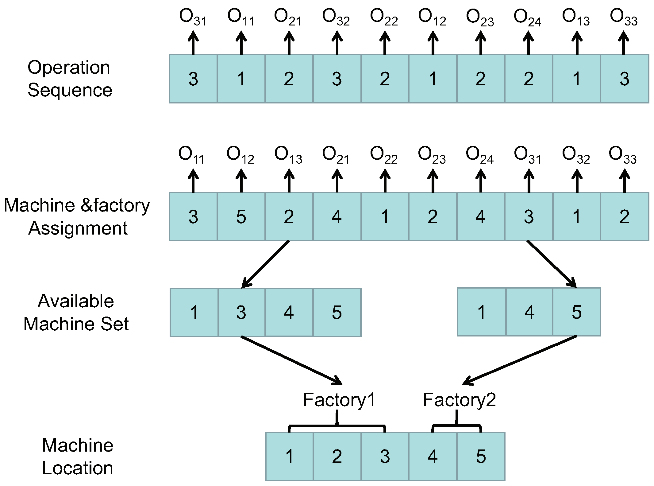
5.2. Encoding and Decoding Method
| Algorithm 2 Insert decoding method |
| Input: An operation sequence vector . |
| Output: A scheduling scheme. |
| 1: while is not empty do |
| 2: The fuzzy transfer time is set to [0,0,0]. |
| 3: Extract the first gene from as . |
| 4: Obtain , , and on of the . |
| 5: if is transferred from another factory then |
| 6: |
| 7: end if |
| 8: if is transferred from another machine in the same factory then |
| 9: |
| 10: end if |
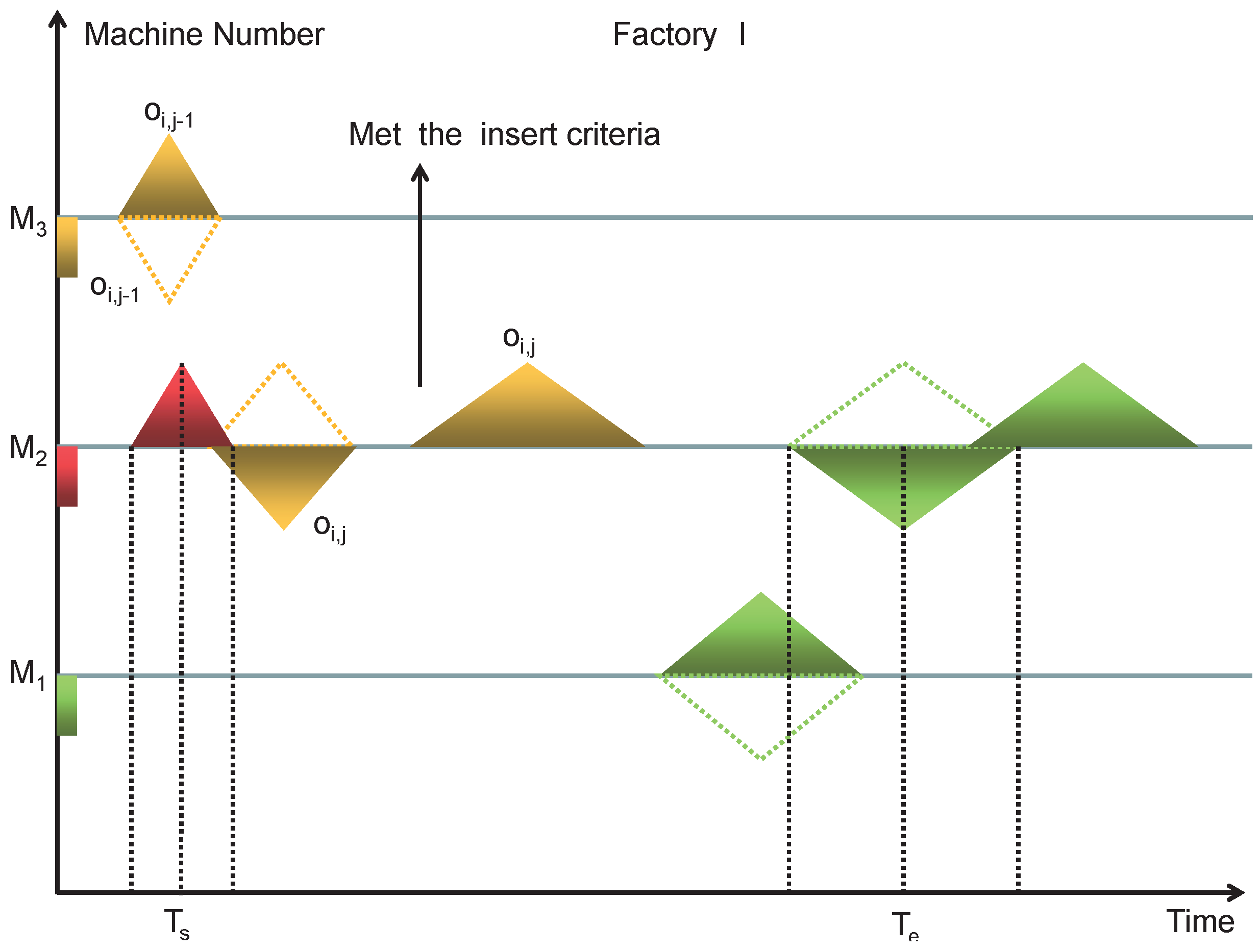
| 11: Obtain all idle time periods of the machine. |
| 12: If the insertion criteria are met, is inserted and the idle time periods are updated. |
| 13: Remove from . |
| 14: end while |
5.3. Population Initialization
- Generate a machine load array to store the total processing time of each machine. The length of the array is the total number of machines. The initial value of the array is set to 0.
- Select a job randomly, and obtain the candidate machine number and fuzzy processing time of each operation of the job.
- According to the operation sequence of the selected job, add the candidate processing time of each operation to the corresponding machine load array, find the lowest value in the array, and store the corresponding machine.
- Update the machine load array, and repeat step 3 until all operations of the selected job are assigned to a machine.
- Select other jobs in the same way until all jobs have been selected.
5.4. Crossover
- Randomly divide the job set into two nonempty sets (Job1,Job2).
- Find the genes belonging to Job1 from Parent1 and copy them to New1 at the same position; find the genes belonging to Job2 from Parent2 and copy them to New2 at the same position.
- Find the genes belonging to Job1 from Parent1 and copy them from left to right to the unassigned positions in New2; find the genes belonging to Job2 from Parent2 and copy them from left to right to the unassigned positions in New1. An example of this procedure is shown in Figure 4.
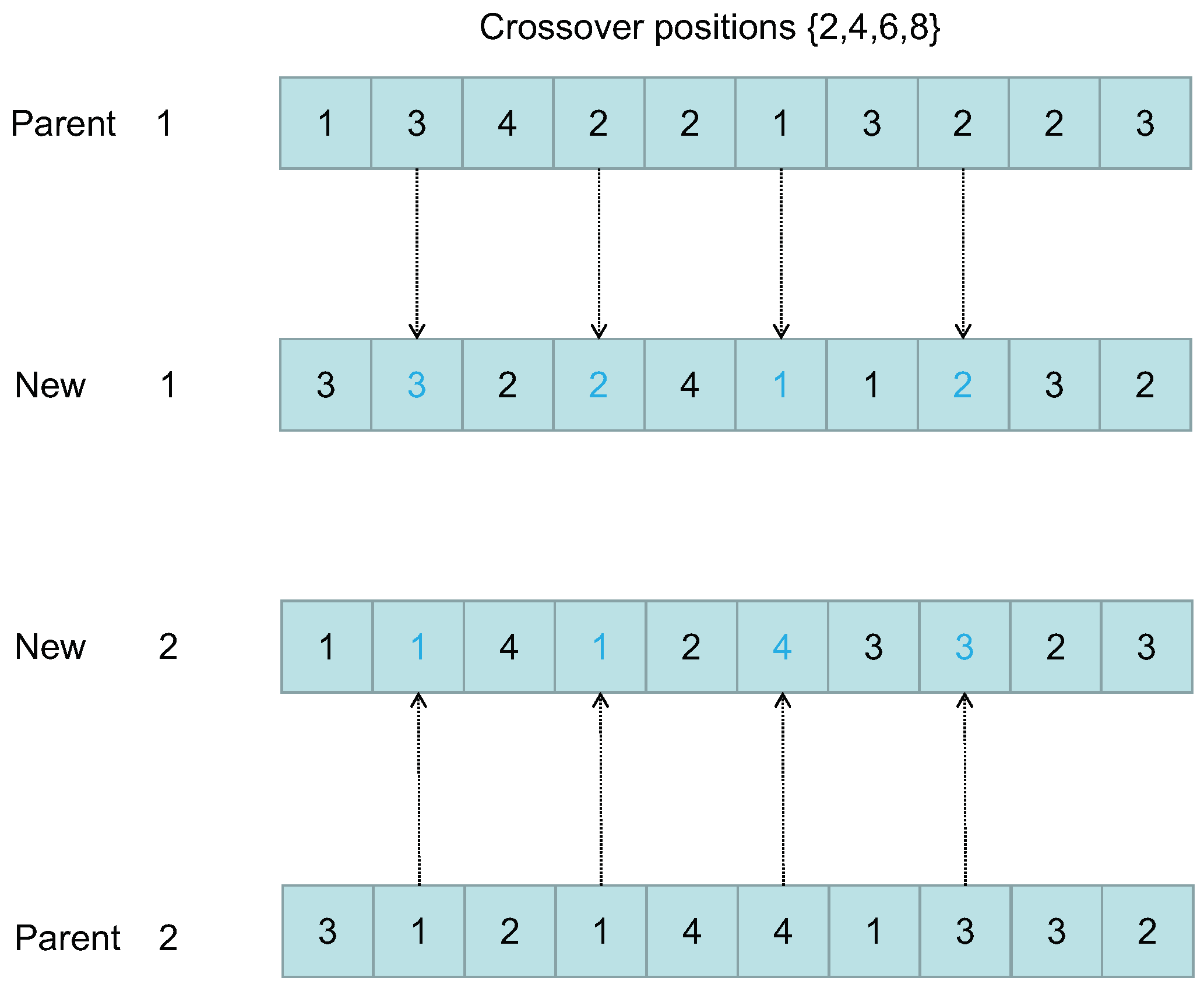
- Randomly generate several positions as crossover positions.
- Exchange the gene values of Parent1 and Parent2 based on the generated crossover positions. An example of this procedure is shown in Figure 5.
5.5. Mutation
- Randomly select two positions, and , in the operation sequence vector.
- Exchange the values of and .
- Randomly select two positions, and , in the equipment allocation vector.
- Obtain , the candidate machine number, and the corresponding fuzzy processing times of and .
- Change the current machine of and to the machine with the minimum fuzzy processing time other than the current machine.
5.6. DVNS
5.6.1. Individual Selection Criteria
- What is the probability of performing local search?
- Which individuals are selected for local search?
| Algorithm 3 High-quality individual selection |
| Input: Current population , local search probability , population size , 300 sets of weight vectors =. |
| Output: High-quality individuals , selected weight vector sets . |
| 1: for to do |
| 2: Randomly select a group of vectors from the set of weight vectors . Calculate according to Equation (15) for each individual, and perform tournament selection to select a high-quality individual. |
| 3: Store the selected individual in and store the selected weight vector set in . |
| 4: end for |
5.6.2. VNS Method
| Algorithm 4 Strategy |
| Input: An individual vector X. |
| Output: Vector after performing local search . |
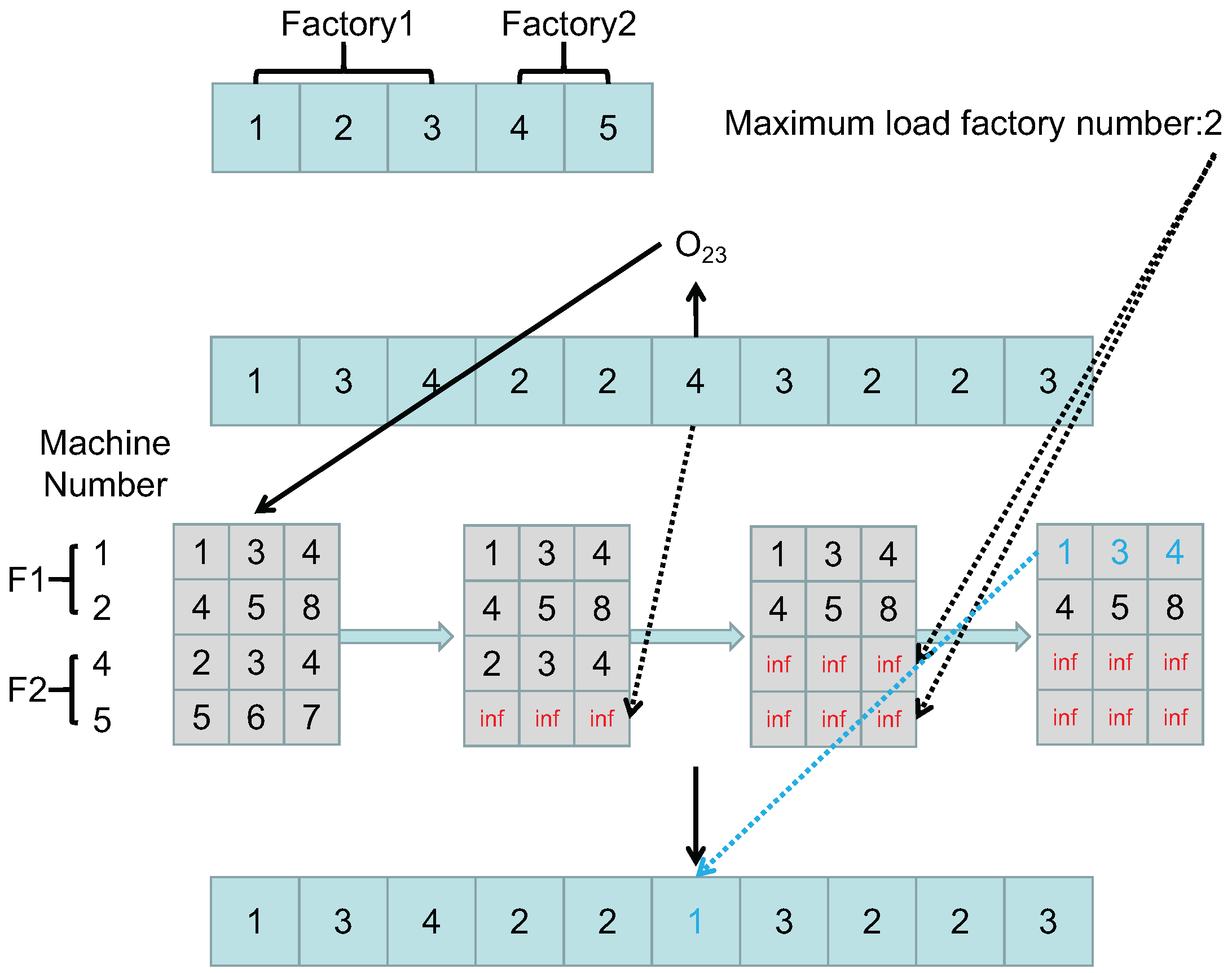
| 1: Decode X and obtain the number of the factory with the maximum load. |
| 2: Obtain the operations processed in factory and store them in set . |
| 3: Randomly select an operation from and obtain its candidate fuzzy processing time array , current gene value and candidate machine index array in . |
| 4: . |
| 5: for i=1 to size do |
| 6: . |
| 7: end for |
| 8: Obtain the minimum value in fuzzy array and its index in . |
| 9: if then |
| 10: Execute Algorithm 5. |
| 11: else |
| 12: Change to . |
| 13: end if |
| Algorithm 5 Strategy |
| Input: An individual vector X. |
| Output: Vector after local search . |
| 1: Randomly select an operation from among all operations. |
| 2: Obtain the candidate fuzzy processing time array and current gene value of . |
| 3: . |
| 4: Obtain the minimum value in fuzzy array and its index in . |
| 5: Change to . |
| Algorithm 6 Strategy |
| Input: An individual vector X. |
| Output: Vector after local search . |
| 1: Obtain the critical path of individual X. |
| 2: Randomly select two positions and from the critical path. |
| 3: Exchange the gene values of and . |
| Algorithm 7 VNS |
| Input: Neighborhood number T, high-quality individual set , selected weight vector sets . |
| Output: Individual sets after the VNS. |
| 1: for to size do |
| 2: . |
| 3: . |
| 4: Decode and calculate () according to Equation (15). |
| 5: . |
| 6: while do |
| 7: for to T do |
| 8: if then |
| 9: Execute Algorithm 4 for to generate . |
| 10: end if |
| 11: if then |
| 12: Execute Algorithm 5 for to generate . |
| 13: end if |
| 14: if then |
| 15: Execute Algorithm 6 for to generate . |
| 16: end if |
| 17: Decode and calculate . |
| 18: . |
| 19: end for |
| 20: Find the minimum value in and its corresponding vector . |
| 21: if then |
| 22: . |
| 23: else |
| 24: . |
| 25: end if |
| 26: end while |
| 27: =. |
| 28: end for |
5.6.3. Acceptance Criteria
| Algorithm 8 DVNS |
| Input: Population . |
| Output: Population after DVNS. |
| 1: Execute Algorithm 3 to select high-quality individuals . |
| 2: Execute Algorithm 7 for to generate individuals after local search. |
| 3: Replace in with to generate . |
6. Experimental Results and Discussion
6.1. Benchmark Construction
- The maximum number of factories is set to [2,3,4] according to the benchmark scale.
- The difference in the number of machines between factories does not exceed 1.
6.2. Performance Metrics
- HV metric:where P denotes the non-dominated solution set generated by the algorithm and denotes the hypercube formed between a solution in the obtained Pareto front and the reference point r. r usually takes the maximum value after the normalization of the objective, i.e., (1, 1, 1), to obtain HV.
- IGD metric:where P denotes the non-dominated solution set generated by the algorithm, P* denotes the Pareto front, and denotes the minimum Euclidean distance between points x and y.
- Spread metric:where the parameters and are the Euclidean distances between the extreme solutions and the boundary solutions of the obtained non-dominated set, denotes the Euclidean distance between consecutive solutions in the obtained non-dominated set of solutions, denotes the average value of , and N denotes the number of non-dominated solution sets.
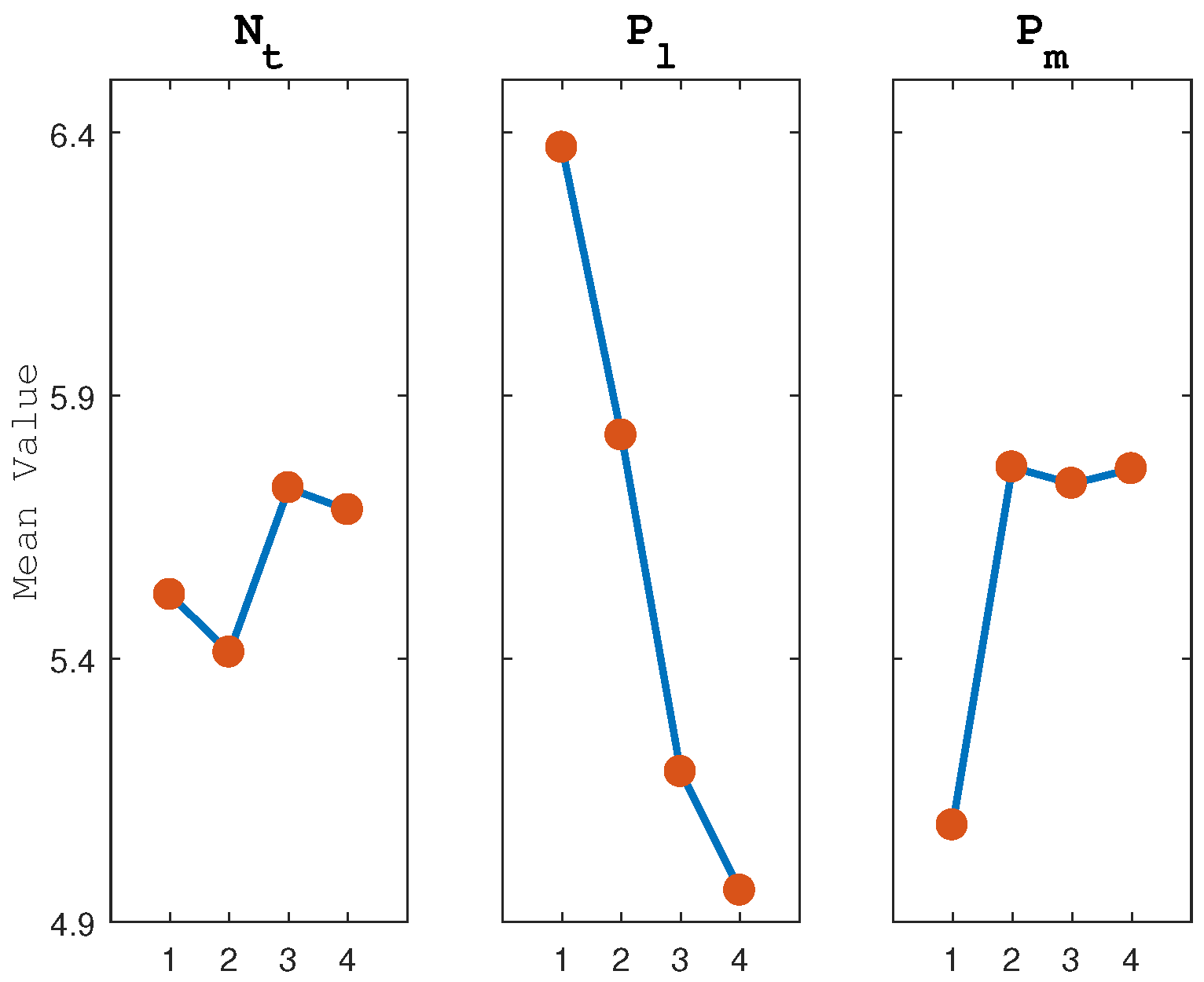
6.3. Parameter Settings
- :
- :
- :
6.4. Effectiveness of the Initialization Strategy
6.5. Effectiveness of the DVNS Strategy
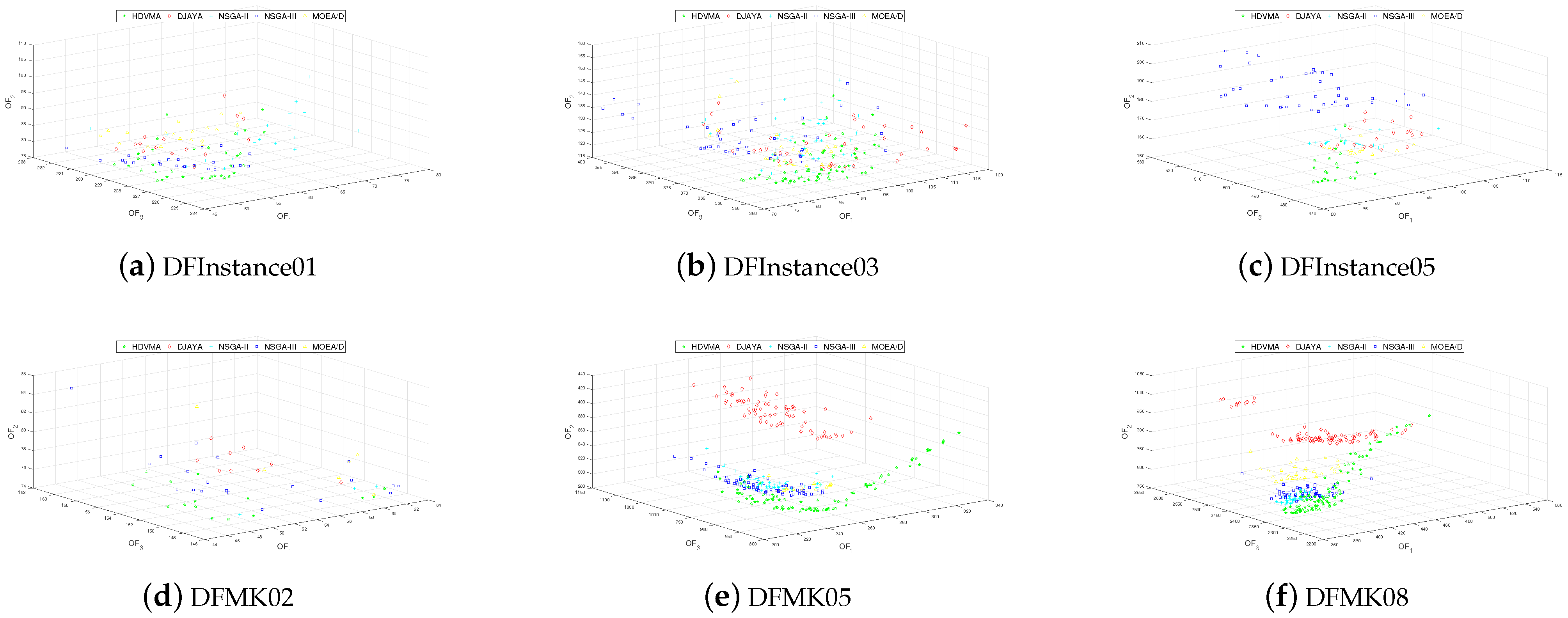
6.6. Comparison with Other Algorithms
7. Conclusions
Author Contributions
Funding
Informed Consent Statement
Data Availability Statement
Conflicts of Interest
References
- Xu, Y.; Sahnoun, M.; Abdelaziz, F.B.; Baudry, D. A simulated multi-objective model for flexible job shop transportation scheduling. Ann. Oper. Res. 2022, 311, 899–920. [Google Scholar] [CrossRef]
- Zhang, Y.; Zhu, H.; Tang, D. An improved hybrid particle swarm optimization for multi-objective flexible job-shop scheduling problem. Kybernetes 2020, 49, 2873–2892. [Google Scholar] [CrossRef]
- Ziaee, M.; Mortazavi, J.; Amra, M. Flexible job shop scheduling problem considering machine and order acceptance, transportation costs, and setup times. Soft Comput. 2022, 26, 3527–3543. [Google Scholar] [CrossRef]
- Deb, K.; Pratap, A.; Agarwal, S.; Meyarivan, T. A fast and elitist multiobjective genetic algorithm: NSGA-II. IEEE Trans. Evol. Comput. 2002, 6, 182–197. [Google Scholar] [CrossRef] [Green Version]
- Naderi, B.; Azab, A. An improved model and novel simulated annealing for distributed job shop problems. Int. J. Adv. Manuf. Technol. 2015, 81, 693–703. [Google Scholar] [CrossRef]
- Chang, H.C.; Liu, T.K. Optimisation of distributed manufacturing flexible job shop scheduling by using hybrid genetic algorithms. J. Intell. Manuf. 2017, 28, 1973–1986. [Google Scholar] [CrossRef]
- Wu, X.; Liu, X.; Zhao, N. An improved differential evolution algorithm for solving a distributed assembly flexible job shop scheduling problem. Memetic Comput. 2019, 11, 335–355. [Google Scholar] [CrossRef]
- Tang, H.; Fang, B.; Liu, R.; Li, Y.; Guo, S. A hybrid teaching and learning-based optimization algorithm for distributed sand casting job-shop scheduling problem. Appl. Soft Comput. 2022, 120, 108694. [Google Scholar] [CrossRef]
- Ziaee, M. A heuristic algorithm for the distributed and flexible job-shop scheduling problem. J. Supercomput. 2014, 67, 69–83. [Google Scholar] [CrossRef]
- Luo, Q.; Deng, Q.; Gong, G.; Zhang, L.; Han, W.; Li, K. An efficient memetic algorithm for distributed flexible job shop scheduling problem with transfers. Expert Syst. Appl. 2020, 160, 113721. [Google Scholar] [CrossRef]
- Sang, Y.; Tan, J. Intelligent factory many-objective distributed flexible job shop collaborative scheduling method. Comput. Ind. Eng. 2022, 164, 107884. [Google Scholar] [CrossRef]
- Sun, L.; Lin, L.; Gen, M.; Li, H. A hybrid cooperative coevolution algorithm for fuzzy flexible job shop scheduling. IEEE Trans. Fuzzy Syst. 2019, 27, 1008–1022. [Google Scholar] [CrossRef]
- Zheng, Y.l.; Li, Y.x.; Lei, D.m. Multi-objective swarm-based neighborhood search for fuzzy flexible job shop scheduling. Int. J. Adv. Manuf. Technol. 2012, 60, 1063–1069. [Google Scholar] [CrossRef]
- Lin, J.; Zhu, L.; Wang, Z.J. A hybrid multi-verse optimization for the fuzzy flexible job-shop scheduling problem. Comput. Ind. Eng. 2019, 127, 1089–1100. [Google Scholar] [CrossRef]
- Li, R.; Gong, W.; Lu, C. Self-adaptive multi-objective evolutionary algorithm for flexible job shop scheduling with fuzzy processing time. Comput. Ind. Eng. 2022, 168, 108099. [Google Scholar] [CrossRef]
- Gao, K.Z.; Suganthan, P.N.; Pan, Q.K.; Tasgetiren, M.F. An effective discrete harmony search algorithm for flexible job shop scheduling problem with fuzzy processing time. Int. J. Prod. Res. 2015, 53, 5896–5911. [Google Scholar] [CrossRef]
- Lin, J. A hybrid biogeography-based optimization for the fuzzy flexible job-shop scheduling problem. Knowl.-Based Syst. 2015, 78, 59–74. [Google Scholar] [CrossRef]
- Gao, K.Z.; Suganthan, P.N.; Pan, Q.K.; Chua, T.J.; Chong, C.S.; Cai, T.X. An improved artificial bee colony algorithm for flexible job-shop scheduling problem with fuzzy processing time. Expert Syst. Appl. 2016, 65, 52–67. [Google Scholar] [CrossRef] [Green Version]
- Vela, C.R.; Afsar, S.; Palacios, J.J.; Gonzalez-Rodriguez, I.; Puente, J. Evolutionary tabu search for flexible due-date satisfaction in fuzzy job shop scheduling. Comput. Oper. Res. 2020, 119, 104931. [Google Scholar] [CrossRef]
- Sakawa, M.; Mori, T. An efficient genetic algorithm for job-shop scheduling problems with fuzzy processing time and fuzzy duedate. Comput. Ind. Eng. 1999, 36, 325–341. [Google Scholar] [CrossRef]
- Lei, D. A genetic algorithm for flexible job shop scheduling with fuzzy processing time. Int. J. Prod. Res. 2010, 48, 2995–3013. [Google Scholar] [CrossRef]
- Xu, W.; Hu, Y.; Luo, W.; Wang, L.; Wu, R. A multi-objective scheduling method for distributed and flexible job shop based on hybrid genetic algorithm and tabu search considering operation outsourcing and carbon emission. Comput. Ind. Eng. 2021, 157, 107318. [Google Scholar] [CrossRef]
- Wang, C.; Tian, N.; Ji, Z.; Wang, Y. Multi-objective fuzzy flexible job shop scheduling using memetic algorithm. J. Stat. Comput. Simul. 2017, 87, 2828–2846. [Google Scholar] [CrossRef]
- Gao, K.Z.; Suganthan, P.N.; Chua, T.J.; Chong, C.S.; Cai, T.X.; Pan, Q.K. A two-stage artificial bee colony algorithm scheduling flexible job-shop scheduling problem with new job insertion. Expert Syst. Appl. 2015, 42, 7652–7663. [Google Scholar] [CrossRef]
- Yuan, Y.; Xu, H. Multiobjective flexible job shop scheduling using memetic algorithms. IEEE Trans. Autom. Sci. Eng. 2013, 12, 336–353. [Google Scholar] [CrossRef]
- Wang, L.; Zhou, G.; Xu, Y.; Wang, S.; Liu, M. An effective artificial bee colony algorithm for the flexible job-shop scheduling problem. Int. J. Adv. Manuf. Technol. 2012, 60, 303–315. [Google Scholar] [CrossRef]
- Lei, D. Co-evolutionary genetic algorithm for fuzzy flexible job shop scheduling. Appl. Soft Comput. 2012, 12, 2237–2245. [Google Scholar] [CrossRef]
- Brandimarte, P. Routing and scheduling in a flexible job shop by tabu search. Ann. Oper. Res. 1993, 41, 157–183. [Google Scholar] [CrossRef]
- Lei, D.; Guo, X. Swarm-based neighbourhood search algorithm for fuzzy flexible job shop scheduling. Int. J. Prod. Res. 2012, 50, 1639–1649. [Google Scholar] [CrossRef]
- Caldeira, R.H.; Gnanavelbabu, A. A Pareto based discrete Jaya algorithm for multi-objective flexible job shop scheduling problem. Expert Syst. Appl. 2021, 170, 114567. [Google Scholar] [CrossRef]


| Jobs | Operations | |||||
|---|---|---|---|---|---|---|
| — | (1,2,3) | (2,3,4) | — | (1,3,5) | ||
| (4,5,6) | (2,3,4) | (5,8,9) | (5,7,8) | (7,9,10) | ||
| (4,5,7) | — | (2,3,4) | (1,2,3) | (8,10,12) | ||
| (4,7,8) | (5,7,10) | (1,2,3) | — | (1,3,5) | ||
| (5,6,7) | (1,2,4) | (8,10,12) | — | (4,5,6) | ||
| (1,3,4) | (4,5,8) | — | (2,3,4) | (5,6,7) | ||
| (1,2,3) | (9,10,11) | — | (6,8,10) | (2,4,5) | ||
| (4,5,6) | — | — | (2,3,4) | (1,3,5) | ||
| — | (12,13,17) | (10,11,13) | (14,15,16) | — | ||
| (5,6,7) | — | (7,9,10) | (10,11,13) | — | ||
| Benchmark | Size (n × f × m) | Source |
|---|---|---|
| DFMK01 | 10 × 2 × 6 | MK01 |
| DFMK02 | 10 × 2 × 6 | MK02 |
| DFMK03 | 15 × 2 × 4 | MK05 |
| DFMK04 | 20 × 2 × 5 | MK07 |
| DFMK05 | 15 × 3 × 8 | MK03 |
| DFMK06 | 15 × 3 × 8 | MK04 |
| DFMK07 | 20 × 3 × 10 | MK08 |
| DFMK08 | 20 × 3 × 10 | MK09 |
| DFMK09 | 10 × 4 × 15 | MK06 |
| DFMK10 | 20 × 4 × 15 | MK10 |
| DFInstance01 | 10 × 3 × 10 | Instance01 |
| DFInstance02 | 10 × 3 × 10 | Instance02 |
| DFInstance03 | 10 × 3 × 10 | Instance03 |
| DFInstance04 | 10 × 3 × 10 | Instance04 |
| DFInstance05 | 15 × 3 × 10 | Instance05 |
| Number | Factor Levels | ODS | ||
|---|---|---|---|---|
| 1 | 1 | 1 | 1 | 5.8898 |
| 2 | 1 | 2 | 2 | 6.0353 |
| 3 | 1 | 3 | 3 | 4.8123 |
| 4 | 1 | 4 | 4 | 5.3476 |
| 5 | 2 | 1 | 2 | 5.7420 |
| 6 | 2 | 2 | 1 | 5.6049 |
| 7 | 2 | 3 | 4 | 5.2423 |
| 8 | 2 | 4 | 3 | 5.0575 |
| 9 | 3 | 1 | 3 | 7.2676 |
| 10 | 3 | 2 | 4 | 5.8657 |
| 11 | 3 | 3 | 1 | 4.5849 |
| 12 | 3 | 4 | 2 | 5.1784 |
| 13 | 4 | 1 | 4 | 6.5863 |
| 14 | 4 | 2 | 3 | 5.7924 |
| 15 | 4 | 3 | 2 | 6.0990 |
| 16 | 4 | 4 | 1 | 4.2528 |
| Benchmarks | HV | IGD | Spread | |||
|---|---|---|---|---|---|---|
| HDVMA-0.15 | HDVMA-0.20 | HDVMA-0.15 | HDVMA-0.20 | HDVMA-0.15 | HDVMA-0.20 | |
| DFMK05 | 0.7011 | 0.7213 | 0.0364 | 0.0350 | 0.6974 | 0.6874 |
| DFInstance02 | 0.6586 | 0.6579 | 0.0515 | 0.0505 | 0.4961 | 0.5171 |
| Benchmarks | HV | IGD | Spread | |||
|---|---|---|---|---|---|---|
| HDVMA-NIS | HDVMA | HDVMA-NIS | HDVMA | HDVMA-NIS | HDVMA | |
| DFMK01 | 0.6471 | 0.6624 | 0.0807 | 0.0797 | 0.4504 | 0.4588 |
| DFMK02 | 0.6486 | 0.6591 | 0.1588 | 0.1442 | 0.7462 | 0.6997 |
| DFMK03 | 0.5682 | 0.6644 | 0.0569 | 0.0317 | 0.6723 | 0.4440 |
| DFMK04 | 0.6196 | 0.6299 | 0.0572 | 0.0531 | 0.4306 | 0.4301 |
| DFMK05 | 0.6517 | 0.7011 | 0.0508 | 0.0364 | 0.7625 | 0.6974 |
| DFMK06 | 0.6578 | 0.7470 | 0.0526 | 0.0341 | 0.6023 | 0.5506 |
| DFMK07 | 0.5490 | 0.6344 | 0.0813 | 0.0622 | 0.4220 | 0.4200 |
| DFMK08 | 0.5386 | 0.7093 | 0.0768 | 0.0436 | 0.6828 | 0.5330 |
| DFMK09 | 0.5549 | 0.5453 | 0.0747 | 0.0775 | 0.5392 | 0.5473 |
| DFMK10 | 0.5360 | 0.6527 | 0.0757 | 0.0664 | 0.4899 | 0.4407 |
| DFInstance01 | 0.5413 | 0.5284 | 0.0844 | 0.0867 | 0.5920 | 0.5656 |
| DFInstance02 | 0.6306 | 0.6586 | 0.0643 | 0.0515 | 0.5057 | 0.4961 |
| DFInstance03 | 0.6609 | 0.6273 | 0.0520 | 0.0491 | 0.5759 | 0.5672 |
| DFInstance04 | 0.6012 | 0.5356 | 0.0909 | 0.1143 | 0.6416 | 0.6853 |
| DFInstance05 | 0.6592 | 0.6293 | 0.0942 | 0.0900 | 0.6022 | 0.5951 |
| Benchmarks | HV | IGD | Spread | |||
|---|---|---|---|---|---|---|
| HDVMA-NLS | HDVMA | HDVMA-NLS | HDVMA | HDVMA-NLS | HDVMA | |
| DFMK01 | 0.5983 | 0.6624 | 0.0960 | 0.0797 | 0.4563 | 0.4588 |
| DFMK02 | 0.5638 | 0.6591 | 0.2009 | 0.1442 | 0.8341 | 0.6997 |
| DFMK03 | 0.6214 | 0.6644 | 0.0422 | 0.0317 | 0.4900 | 0.4440 |
| DFMK04 | 0.5923 | 0.6299 | 0.0512 | 0.0531 | 0.4662 | 0.4301 |
| DFMK05 | 0.7110 | 0.7011 | 0.0378 | 0.0364 | 0.7177 | 0.6974 |
| DFMK06 | 0.6873 | 0.7470 | 0.0444 | 0.0341 | 0.6076 | 0.5506 |
| DFMK07 | 0.6269 | 0.6344 | 0.0698 | 0.0622 | 0.3866 | 0.4200 |
| DFMK08 | 0.6968 | 0.7093 | 0.0510 | 0.0436 | 0.5650 | 0.5330 |
| DFMK09 | 0.4200 | 0.5453 | 0.1341 | 0.0775 | 0.6358 | 0.5473 |
| DFMK10 | 0.5898 | 0.6527 | 0.1087 | 0.0664 | 0.4608 | 0.4407 |
| DFInstance01 | 0.3806 | 0.5284 | 0.1175 | 0.0867 | 0.6412 | 0.5656 |
| DFInstance02 | 0.5010 | 0.6586 | 0.1572 | 0.0515 | 0.5368 | 0.4961 |
| DFInstance03 | 0.5194 | 0.6273 | 0.0852 | 0.0491 | 0.6008 | 0.5672 |
| DFInstance04 | 0.4135 | 0.5356 | 0.1553 | 0.1143 | 0.7287 | 0.6853 |
| DFInstance05 | 0.5087 | 0.6293 | 0.1455 | 0.0900 | 0.6037 | 0.5951 |
| Benchmarks | NSGA-II | NSGA-III | MOEA/D | DJAYA | HDVMA |
|---|---|---|---|---|---|
| DFMK01 | 0.5690 | 0.6106 | 0.4775 | 0.5037 | 0.6624 |
| DFMK02 | 0.4793 | 0.5012 | 0.2522 | 0.2757 | 0.6847 |
| DFMK03 | 0.4577 | 0.4981 | 0.2799 | 0.4788 | 0.6644 |
| DFMK04 | 0.4748 | 0.4509 | 0.3378 | 0.2815 | 0.6447 |
| DFMK05 | 0.2483 | 0.2801 | 0.0860 | 0.1620 | 0.7011 |
| DFMK06 | 0.4946 | 0.4853 | 0.4239 | 0.4778 | 0.7401 |
| DFMK07 | 0.4440 | 0.4370 | 0.3338 | 0.2564 | 0.6273 |
| DFMK08 | 0.2654 | 0.3173 | 0.1439 | 0.1587 | 0.7145 |
| DFMK09 | 0.1958 | 0.2890 | 0.0695 | 0.1337 | 0.5883 |
| DFMK10 | 0.1862 | 0.2275 | 0.1009 | 0.1157 | 0.6613 |
| DFInstance01 | 0.4604 | 0.4199 | 0.3707 | 0.4829 | 0.5456 |
| DFInstance02 | 0.5426 | 0.4514 | 0.3451 | 0.5537 | 0.6841 |
| DFInstance03 | 0.5516 | 0.4268 | 0.3691 | 0.5437 | 0.6369 |
| DFInstance04 | 0.5217 | 0.4657 | 0.3623 | 0.4904 | 0.6527 |
| DFInstance05 | 0.2718 | 0.2150 | 0.1356 | 0.3637 | 0.6293 |
| Benchmarks | NSGA-II | NSGA-III | MOEA/D | DJAYA | HDVMA |
|---|---|---|---|---|---|
| DFMK01 | 0.0771 | 0.0792 | 0.1388 | 0.1746 | 0.0565 |
| DFMK02 | 0.1516 | 0.1444 | 0.2408 | 0.2796 | 0.0814 |
| DFMK03 | 0.0608 | 0.0717 | 0.1767 | 0.1817 | 0.0228 |
| DFMK04 | 0.0640 | 0.0734 | 0.0982 | 0.3528 | 0.0362 |
| DFMK05 | 0.1745 | 0.1653 | 0.2160 | 0.4757 | 0.0165 |
| DFMK06 | 0.0860 | 0.1072 | 0.1256 | 0.1695 | 0.0301 |
| DFMK07 | 0.0835 | 0.0805 | 0.1166 | 0.2508 | 0.0620 |
| DFMK08 | 0.1891 | 0.2008 | 0.2828 | 0.5683 | 0.0214 |
| DFMK09 | 0.1786 | 0.1929 | 0.2393 | 0.5937 | 0.0266 |
| DFMK10 | 0.2233 | 0.2375 | 0.3141 | 0.5948 | 0.0310 |
| DFInstance01 | 0.0862 | 0.1212 | 0.1341 | 0.1537 | 0.0323 |
| DFInstance02 | 0.0962 | 0.1405 | 0.1421 | 0.1463 | 0.0311 |
| DFInstance03 | 0.0714 | 0.1336 | 0.1322 | 0.1328 | 0.0303 |
| DFInstance04 | 0.1161 | 0.2346 | 0.1589 | 0.1863 | 0.0614 |
| DFInstance05 | 0.2242 | 0.4316 | 0.2589 | 0.2864 | 0.0241 |
| Benchmarks | NSGA-II | NSGA-III | MOEA/D | DJAYA | HDVMA |
|---|---|---|---|---|---|
| DFMK01 | 0.4735 | 0.4803 | 0.4507 | 0.4762 | 0.4770 |
| DFMK02 | 0.7896 | 0.8015 | 1.0096 | 0.8362 | 0.7210 |
| DFMK03 | 0.7414 | 0.7280 | 0.8923 | 0.6290 | 0.4697 |
| DFMK04 | 0.4741 | 0.4727 | 0.5453 | 0.6106 | 0.4195 |
| DFMK05 | 0.8243 | 0.7590 | 0.9287 | 0.7388 | 0.6807 |
| DFMK06 | 0.6696 | 0.6749 | 0.7724 | 0.6337 | 0.5532 |
| DFMK07 | 0.4775 | 0.4692 | 0.5123 | 0.6303 | 0.4104 |
| DFMK08 | 0.7885 | 0.7316 | 0.7985 | 0.7186 | 0.5616 |
| DFMK09 | 0.7554 | 0.6602 | 0.9057 | 0.7420 | 0.6903 |
| DFMK10 | 0.6329 | 0.6540 | 0.8001 | 0.7662 | 0.4421 |
| DFInstance01 | 0.7162 | 0.7481 | 0.8170 | 0.7309 | 0.6127 |
| DFInstance02 | 0.6890 | 0.7571 | 0.7912 | 0.7023 | 0.6523 |
| DFInstance03 | 0.7486 | 0.7310 | 0.8653 | 0.6954 | 0.6608 |
| DFInstance04 | 0.7407 | 0.6880 | 0.8415 | 0.7038 | 0.6959 |
| DFInstance05 | 0.7727 | 0.8001 | 0.9189 | 0.7725 | 0.6572 |
Publisher’s Note: MDPI stays neutral with regard to jurisdictional claims in published maps and institutional affiliations. |
© 2022 by the authors. Licensee MDPI, Basel, Switzerland. This article is an open access article distributed under the terms and conditions of the Creative Commons Attribution (CC BY) license (https://creativecommons.org/licenses/by/4.0/).
Share and Cite
Yang, J.; Xu, H. Hybrid Memetic Algorithm to Solve Multiobjective Distributed Fuzzy Flexible Job Shop Scheduling Problem with Transfer. Processes 2022, 10, 1517. https://doi.org/10.3390/pr10081517
Yang J, Xu H. Hybrid Memetic Algorithm to Solve Multiobjective Distributed Fuzzy Flexible Job Shop Scheduling Problem with Transfer. Processes. 2022; 10(8):1517. https://doi.org/10.3390/pr10081517
Chicago/Turabian StyleYang, Jinfeng, and Hua Xu. 2022. "Hybrid Memetic Algorithm to Solve Multiobjective Distributed Fuzzy Flexible Job Shop Scheduling Problem with Transfer" Processes 10, no. 8: 1517. https://doi.org/10.3390/pr10081517
APA StyleYang, J., & Xu, H. (2022). Hybrid Memetic Algorithm to Solve Multiobjective Distributed Fuzzy Flexible Job Shop Scheduling Problem with Transfer. Processes, 10(8), 1517. https://doi.org/10.3390/pr10081517