Article

Optimization of Two-Dimensional Extended Warranty Scheme for Failure Dependence of a Multi-Component System with Improved PSO–BAS Algorithm

1
Shijiazhuang Campus of Army Engineering University of PLA, 97 Heping West Road, Ning’an Street, Xinhua District, Shijiazhuang 050003, China
2
Hebei Key Laboratory of Condition Monitoring and Assessment of Mechanical Equipment, Shijiazhuang 050003, China
*
Author to whom correspondence should be addressed.
Processes 2022, 10(8), 1479; https://doi.org/10.3390/pr10081479
Submission received: 1 July 2022 / Revised: 20 July 2022 / Accepted: 21 July 2022 / Published: 28 July 2022
(This article belongs to the Section Automation Control Systems)

Abstract

:
Human society is entering the era of Industry 4.0; engineering systems are becoming more complex, which increases the difficulties of maintenance support work. Failure dependence exists widely in multi-component systems. In this work, a model of two-dimensional (2D) warranty decision making was constructed by using a failure-dependence analysis for multi-component systems and by considering the extended warranty cost and the system availability. The decision was to cut the warranty cost as much as possible for manufacturers, while the constraint condition was the minimum acceptable availability for the customer. The model combined preventive maintenance as well as corrective maintenance strategies. Under the condition that the multi-component system is replaced upon the expiration of the extended warranty (EW), the optimal 2D EW duration and preventive maintenance interval could be obtained through the model. In a case analysis, the optimal EW scheme for the gearbox of an electric multiple unit (EMU) system was obtained by using a grid search algorithm, a PSO algorithm, and a PSO–BAS algorithm. Through comparison, the PSO–BAS algorithm obtained a better scheme with lower warranty costs and higher system availability. A comparative analysis and a sensitivity analysis showed that the model provides a theoretical basis for manufacturers to optimize their 2D extended gearbox warranties.

1. Introduction

A multi-component system is made up of multiple subsystems or components that are interrelated and that affect each other in order to complete specific functions together. In the era of Industry 4.0, more and more modern technical systems are widely used in the fields of production, industrial manufacturing, and military [1]. For example, an electric multiple unit (EMU) system, which is a type of modern train and which is composed of several vehicles with power (motor cars) and vehicles without power (trailers), has complex structures and high integration. EMUs are usually composed of many multi-component systems, and there is failure dependence among components in the system, which greatly increases the difficulty of maintenance and daily management. The gearbox is an important subsystem of an EMU system, which is mainly composed of bearings and gears. There is failure dependence between the bearings and the gears, which is mainly reflected by bearing failures that lead to the increased vibration of the gearbox, which accelerates the gear wear process and increases the gear failure rate. The existence of failure dependence makes it more difficult to develop a warranty plan for the gearbox.
Two-dimensional (2D) warranty means that the warranty period is composed of two dimensions. Usually, one dimension represents calendar time and the other represents usage intensity. An extended warranty (EW) refers to a warranty service contract signed between the manufacturers and the customers following the expiration of the basic warranty [2]. The manufacturer provides follow-up service work for a certain period, and the user needs to pay for it. Nowadays, the reliability of products is becoming higher and higher, and the service life is becoming longer and longer. A basic warranty can no longer meet the needs of users. Therefore, EWs are becoming more and more common. The main reason why users choose an EW is that they hope the failure of the product beyond the basic warranty period can be repaired in time, so as to ensure that the product remains available. At present, providing an EW has become an important way for manufacturers to make profits [3]. Manufacturers hope to make the EW cost of multi-component systems as low as possible during the EW period, but users hope to obtain higher availability [4]. Therefore, in the research of EWs, it is crucial to scientifically formulate an EW scheme by considering the demands of both the users and the manufacturers.
A warranty scheme usually includes the determination of a warranty period and a preventive maintenance interval. In a model, these indicators usually exist in the form of decision variables. Therefore, the process of obtaining the optimal scheme is the process of optimizing the decision variables. The grid search method is an optimization algorithm often used in maintenance optimization [5]. The function of a grid search is to discretize the continuous variables within a specified range, divide them into a limited number of variable values according to the set grid density (or step size), and then respectively substitute the current values of variables into the model to calculate the objective function values at that time. This method is suitable for optimization problems with few variables. Usually, the number of variables should not be too large. Too many variables can lead to a combination explosion, and the time complexity of the algorithm will increase exponentially. As one of the methods for solving global optimization as well as multivariable optimization problems, the particle swarm optimization (PSO) algorithm has been extensively applied to various planning problems and has also been extensively adopted in the field of warranty decision making [6,7,8]. The advantage of the PSO algorithm is that its function makes it easier to find the global optimal value without becoming trapped in a local optimal value. The disadvantage is that the settings of inertia weight and the learning factor have a great impact on the result. In addition, the traditional PSO algorithm usually treats a particle as a mass point; that is, it has no orientation. The beetle antennae search (BAS) algorithm was put forward by Jiang et al. in 2017 [9], and its principle is based on the observation that a beetle will change its flight direction according to the different odor intensities perceived by the left and right antennae when hunting. The BAS algorithm has the characteristics of fast searching and simple execution. It is a monomer search algorithm that has great advantages for dealing with low-dimensional optimization objectives, but it is easy to fall into local extremes during multimodal complex function optimization. In this paper, a PSO–BAS algorithm is proposed by adopting the traditional PSO algorithm while regarding the particle as a beetle. Before each particle position iteration, the particle will first change its orientation according to the different smell intensities perceived by the left and right antennae, so as to make it faster to find the global optimal solution. A case study is provided to prove this conjecture.
The main research work of the present article is:
(1)
For a multi-component system with unidirectional failure dependence, the present study attempts to develop a failure rate model through a failure-dependence analysis for the system. The protocols for both preventive (imperfect) maintenance and corrective (minimum) maintenance are introduced, and their repair effects are described using the virtual age method and minimum maintenance theory, respectively. Meanwhile, the non-homogeneous Poisson process (NHPP) theory was adopted for establishing a model for the number of system failures in a period of time, which provides an important basis for the model of warranty cost and for system availability.
(2)
For a failure-dependence system with a 2D warranty, under the case that the system is replaced when the warranty expires, models of warranty cost per unit time and the availability were established. In the case study, an optimal 2D EW scheme for the gearbox of an EMU system was determined via the PSO–BAS algorithm, with the minimum warranty cost as the decision objective and the availability acceptable to users as the constraint. The warranty scheme (decision variables) included the optimal 2D EW period and the preventive maintenance interval.
The remainder of this article is structured as follows. Research closely related to this study is analyzed in Section 2. Section 3 illustrates a description of the optimization model and its assumptions. Based on the failure rate model, Section 4 of this paper presents the constructed models for the warranty cost and the system availability. Section 5 is the case analysis, and Section 6 is the conclusion of the present study. Future research is also proposed in Section 6.

2. Related Work

2.1. 2D Warranty

The 2D warranty policy has, in fact, been widely used for modern technical equipment, such as automobiles and aircraft engines. The warranty area of a 2D warranty is usually represented by a 2D plane, in which one dimension represents calendar time and the other dimension represents usage. Wang [10] introduced in detail the 2D warranty policy and its corresponding warranty area shape, and provided a more comprehensive overview of the 2D warranty. Compared with one-dimensional warranties, a 2D warranty additionally considers the system’s degradation in the usage process, so it is more in-line with the failure law of the system. Meanwhile, when the deadline for one of the dimensions is reached, the warranty will end, which can reduce the warranty pressure on the manufacturers to a certain extent. Research on 2D warranties is conducted as follows. First, the 2D warranty area is divided into multiple subareas; then, the maintenance strategy is determined; and finally, the optimal 2D warranty scheme is obtained using a decision-making goal of warranty cost [11], availability [12], cost-effectiveness ratio [13], etc. The authors of [14,15,16,17] studied 2D warranties according to the above process and modeled them according to different optimization objectives. In recent years, 2D warranty research has shown some new trends. Peng [18] developed a random and dynamic maintenance model by changing the utilization rate. The authors of [19] used a value–risk approach for dual-channel sales manufacturers while optimizing a 2D warranty policy and the pricing (with dual-channel products referring to products sold online and offline simultaneously). By completely taking the heterogeneity of users into consideration, the authors of [20,21,22] customized 2D warranty services for different customers. The authors of [23,24,25] adopted preventive maintenance measures into 2D warranty services with the purpose of reducing warranty costs and improving availability. Based on key information obtained from historical claim data, the authors of [26,27,28] investigated a data-driven 2D warranty decision model. In accordance with the literature review, it can be observed that currently, studies on 2D warranties have gradually highlighted customer heterogeneity, focusing on the personalization of warranty schemes for customers through their different usage behaviors. At the same time, the diversity of products and warranty claim data are receiving more and more attention in the warranty decision-making process. Meanwhile, because preventive maintenance can diminish losses from a system shutdown and avoid severe consequences from failures, there are more and more studies on 2D warranties based on preventive maintenance. Compared with one-dimensional warranties, a 2D warranty involves more complex modeling, so most of the existing studies have only considered a single component; multiple-component dependence has rarely been considered.

2.2. Extended Warranty

Most studies on EWs have set the minimum warranty cost or the highest profit margin of manufacturers as the decision goal, and they fail to focus on the users. For example, Tong [29] studied the best degree of maintenance within an EW duration while considering a changing utilization rate, with the goal of lowering the warranty cost. By comprehensively considering the influence of engineering factors and market factors on the 2D EW price, Wang [30] derived the best product price and 2D EW cost so that the profit margin of manufacturers could be expanded. Xin [31] established a warranty cost model based on the failure history of products and the usage rate by users, and determined the optimal warranty price based on the manufacturer’s expected warranty cost and profit. Based on the assumption that not all users will purchase an extended warranty, the author of [3] jointly optimized the basic warranty period, extended warranty period, product price, and extended warranty cost. These studies are of great significance for making EW decisions for a manufacturer, but they minimize the interests of users to a certain extent. Based on the above analysis, our goal was to establish an EW decision model that comprehensively considers the EW cost together with the multi-component system availability.

2.3. Availability

Availability refers to the probability that a multi-component system is in a usable state when it starts to perform tasks at any random time. Availability is one of the important parameters that affect users. In the field of maintenance decision making, the availability of equipment has been extensively studied. Some studies have only considered the impact of availability on maintenance decision making. For example, Yang [32] took the maximum average availability of a system as the decision-making goal and obtained the optimal preventive maintenance interval. Henry et al. [33] compared the availability of a power generation system under reliability-centered maintenance (RCM), risk-based maintenance (RBM), condition-based maintenance (CBM), and a combination of the three maintenance strategies. However, these studies did not consider the impact of the maintenance cost on decision making. Meanwhile, it has been found that some studies have paid attention to both the availability and the maintenance cost. For example, Qiu [34] considered both the maintenance cost and the system availability, and studied the optimal failure detection and imperfect maintenance strategy of a remote power supply system; Ahn [35] studied the optimal preventive maintenance interval for minimizing the maintenance cost on the premise of ensuring the availability of an engineering system. Research considering both the warranty cost and the availability in two-dimensional warranty decision making has been conducted by the authors of [36,37,38]. However, there are few studies on 2D warranties that consider the warranty cost and the availability with multi-component failure dependence.

2.4. The Failure Dependence

In the existing research, mainly three types of dependence among multiple components have been considered: structural dependence, economic dependence, and failure dependence. Failure dependence exists widely in multi-component systems, and it has attracted extensive attention in academia. Failure dependence describes the characteristics of failure interactions between internal components of a system [39]. The failure dependence among multiple components can be categorized into three types [40]: fault correlation (Type I, which implies that the failure of a certain component is responsible for the failure of other components with a certain probability); failure rate correlation (Type II, which involves the failure of one component increasing the failure rate of other components); and impact damage correlation (Type III, which involves the failure of one component causing random degradation to other components). Sun [41] introduced the derivation method of the failure-dependence coefficient between components based on an experiment. Zhang [42] studied the periodic inspection strategy of a Type I failure-dependent k-out-of-n system. Based on an analysis of Type II failure dependence, the authors of [43,44,45] studied the optimal maintenance scheme of a system. Among them, the authors of [43] comprehensively considered Type I failure dependence and Type II failure dependence. The research on failure dependence in multi-component systems is still limited to maintenance decision making, without considering the impact of different warranty methods on the maintenance cost and maintenance plan. In terms of the multi-component system studied in this paper, its components exhibit failure dependence in engineering practices. Based on a 2D warranty, this paper considers the failure dependence between multiple components, and EW decision making is the focus of this paper.

3. Model Description and Assumptions

3.1. Failure-Dependence Analysis

Based on the comprehensive consideration of Type I failure dependence and Type II failure dependence, a multi-component failure-dependence model has been analyzed in detail by the authors of [43]. This paper mainly relies on the analysis results of [43] to establish the model. Figure 1 shows the failure influence path of a four-component system.
For a failure-dependent multi-component system, each component’s real failure rate comprises the individual and associated failure rates. The individual failure rate is usually fixed in the design stage and cannot be changed in the practical stage, whereas the associated failure rate usually results from other components [46]; both the failure-dependence coefficient and the number of failures will affect the associated failure rate. In terms of a system consisting of q components, each component’s real failure rate is given by the following equation [43]:
λ a ( t | r ) = λ a 0 ( t | r ) + b [ θ a b ( t | r ) ] [ m b λ a b ( t | r ) 2 ]
where λ a ( t | r ) represents the actual failure rate of a single component; 1 a q and a N + ; λ a 0 ( t | r ) represent each component’s individual failure rate; λ a b ( t | r ) represents the associated failure rate caused by component b on component a , with b { b | b = 1 , 2 , 3 , , q   a n d   b a } ; and θ a b ( t | r ) represents the failure impact factor of component b on component a , with 0 θ a b ( t | r ) 1 . When θ a b ( t | r ) equals 0, it indicates that no correlation exists between the components, and when θ a b ( t | r ) equals 1, it indicates that component b ’s failure will eventually result in the failure of component a . The variable m b represents the number of failures of component b at a given time. Since the failure of component b affects both itself and component a, the denominator in Equation (1) is 2.

3.2. Model Description

A two-component failure-dependence system has been taken as an example. The system is comprised of a key component and the subsystem. Due to the short service time during the basic warranty period, the failure rate is low. At this time, the use of preventive maintenance will cause excess maintenance and increase the warranty cost. Therefore, within the duration of a basic warranty, corrective maintenance is implemented for the system, whereas preventive maintenance is implemented in the EW period. For the key component and the subsystem, their respective failure rates are represented as λ ψ ( t | r ) and λ s ( t | r ) . Key component failure leads to an elevation in the subsystem failure rate (related to type I failure dependence). The minimum maintenance is the total of all corrective maintenance. The decision variables are the preventive maintenance interval and the EW period. The decision goal is to obtain the lowest warranty cost per unit time, and the constraint is the availability. Through a case analysis, the optimal 2D EW scheme of the gearbox is obtained.

3.3. Model Assumptions

The assumptions on which the model is based are as follows:
(1)
The components of the system are connected in series;
(2)
The failure rate of the components increases with time and utilization rate;
(3)
The preventive maintenance cost does not alter with the preventive maintenance time;
(4)
The cost for a single corrective maintenance action does not change with the time and frequency of the maintenance, and the component failure rate is not altered by such maintenance.

4. Optimization Model Construction

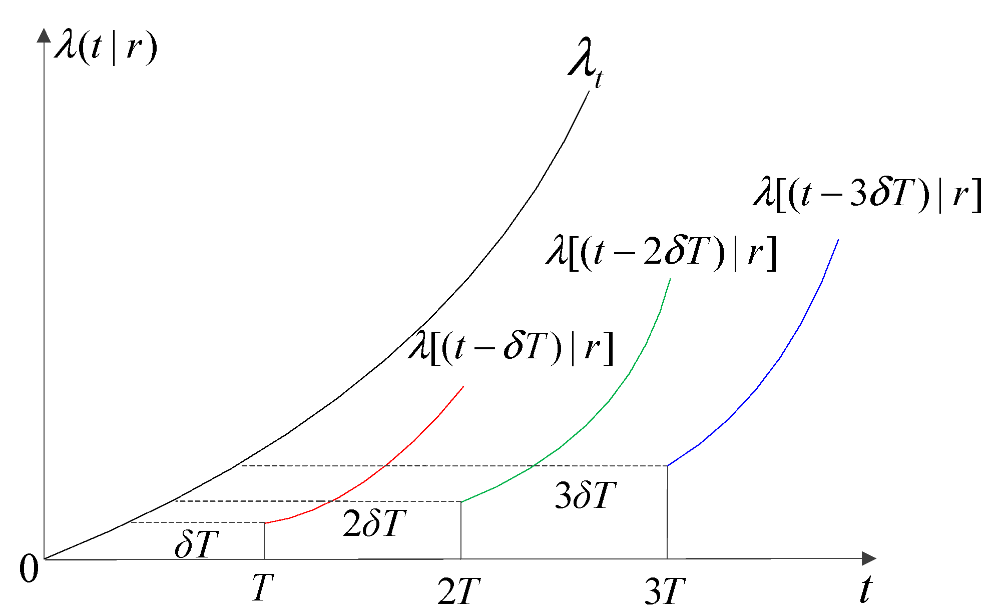
4.1. Failure Rate Model

Generally, the reliability of a system is closely related to the utilization rate. In the design stage, the reliability index is designed under a specific utilization rate. Therefore, in the usage stage, a change in the utilization rate will inevitably lead to a change in the reliability and failure rate. Based on this concept, this paper constructs the failure rate function of components based on the accelerated failure time (AFT) model. Lawless [47] exploited the accelerated failure time and proportional hazards models to investigate the impact of utilization rate on system failure. The main assumption of the accelerated failure time model is that the failure time is inversely proportional to the applied stress; that is, the failure time of products under high stress is shorter than that of products under low stress. It also assumes that the failure time distribution has the same form. In other words, if the failure time of a product under high stress is an exponential distribution, then the failure time under low stress is also an exponential distribution. The present method has a theoretical foundation, and it has been extensively applied.
Assuming that T s and T r respectively represent the time to the first failure based on the design rate of utilization r s and the real rate of utilization r , the computational formula for their association is [36]:
T r T s = ( r s r ) γ
Suppose F s ( t ; α s , φ ) refers to the function of the cumulative distribution for failure under r s , in which α s and φ respectively denote the scale parameter and shape parameter of the failure distribution under the design utilization rate. For the actual utilization rate r , the scale parameter of the cumulative failure distribution function of the system is [36]:
α r = α s ( r s r ) γ
where the AFT parameter γ 1 . Based on this, for the utilization rate r , the cumulative failure distribution function of the system can be written as [36]:
F ( t ; α r , φ ) = F s ( t ; α s ( r s r ) γ , φ )
Due to the fact that the shape parameter does not alter with the utilization rate, it is neglected in the following expression. For the utilization rate r , the failure rate function of the system is expressed as [36]:
λ ( t | r ) = λ ( t ; α r ) = f ( t ; α r ) F ¯ ( t ; α r )

4.2. Imperfect Preventive Maintenance Strategy

Within the EW period, periodic imperfect preventive maintenance is adopted for the components. The degrees of repair for imperfect preventive maintenance range from “bad as old” to “good as new” [48]. This paper adopts the virtual age method for describing the effects of imperfect preventive maintenance [49,50,51]. δ is the improvement coefficient of preventive maintenance. The failure rate for the system at the kth preventive maintenance interval can be depicted as:
λ ( t | r ) = λ [ ( t δ ( k 1 ) T ) | r ]
where T refers to the interval of preventive maintenance. The change in the component failure rate after each imperfect preventive maintenance is shown in Figure 2.

4.3. Corrective Maintenance Strategy

The corrective maintenance (minimum maintenance) strategy is adopted for the failure of components. A characteristic of minimum maintenance is that the NHPP (non-homogeneous Poisson process) is obeyed by failures [30,52]. For the component, its anticipated number of failures over a period of time can be deduced as:
E [ N ( t | r ) ] = 0 t λ ( s | r ) d s
where N ( t | r ) indicates the number of component failures in [ 0 , t ] , and λ ( s | r ) signifies the component failure rate.

4.4. 2D EW Cost Model
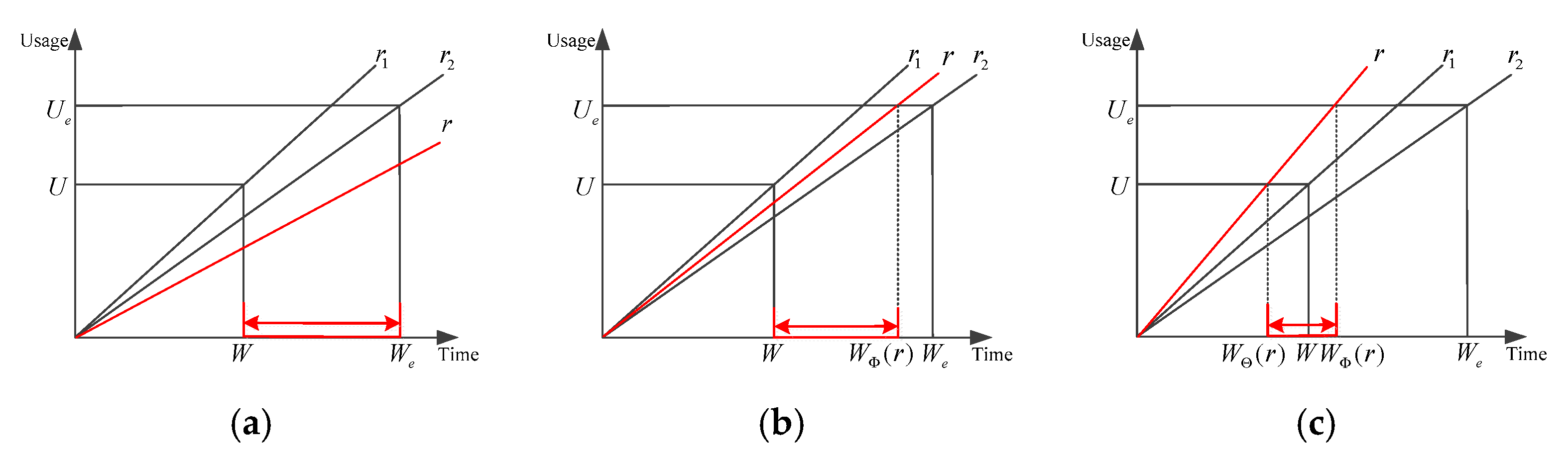
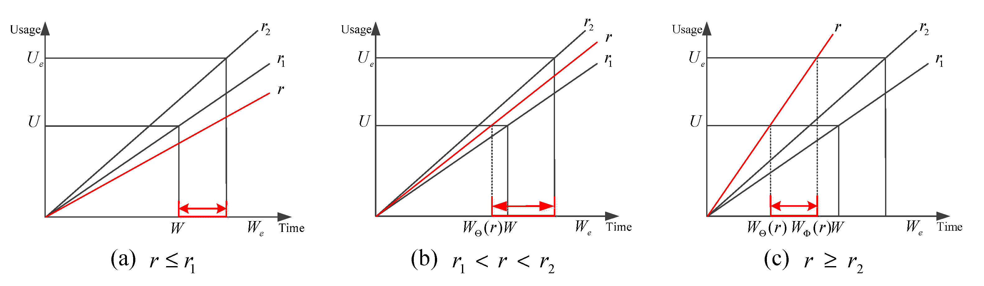
The duration of EW in the time dimension and usage dimension is denoted as W e and U e , respectively. The duration of the basic warranty in the time dimension and usage dimension is denoted as W and U, respectively. Then, according to assumption (6), the shape parameters r 2 and r 1 of the EW area and the basic warranty area, respectively, are:
r 2 = U e W e ,   r 1 = U W
For the studied system, the number of imperfect preventive maintenance activities during the EW duration is:
n = f l o o r { [ W Φ ( r ) W Θ ( r ) ] / ( T + T p ) }  
where “ f l o o r ( ) ” represents the rounding down function; T p represents the time required for imperfect preventive maintenance; W Φ ( r ) indicates the end time of the EW period for the utilization rate r ; and W Θ ( r ) indicates the start time of the EW period for the utilization rate r . The values of W Φ ( r ) and W Θ ( r ) are decided by the value of r , as shown in Figure 3 and Figure 4.
As shown in Figure 3, when r 2 r 1 , W Θ ( r ) and W Φ ( r ) are piecewise functions with r:
W Θ ( r ) = { W r l r r 1 U r   r 1 r r u
W Φ ( r ) = { W e r l r r 2 U e r r 2 r r u
where r l and r u are the minimum and maximum utilization rates, respectively.
Similarly, when r 2 > r 1 , the 2D EW period of the multi-component system is shown in Figure 4.
As shown in Figure 4, when r 2 > r 1 , W Θ ( r ) and W Φ ( r ) are piecewise functions with r:
W Θ ( r ) = { W r l r r 1 U r   r 1 r r u
W Φ ( r ) = { W e r l r r 2 U e r r 2 r r u
Within the EW period, the 2D EW cost for the studied system is mostly composed of two parts: the preventive maintenance cost and the minimum maintenance cost. It can be written as:
E C [ T , W Φ ( r ) , W Θ ( r ) ] = n C p + k = 1 n E C f k ( T ) + E C f [ W Θ ( r ) + n ( T + T p ) , W Φ ( r ) ]
where T is the interval of preventive (imperfect) maintenance, and E C f k ( T ) denotes the anticipated minimum expenditure for maintenance in the k th preventive maintenance interval. E C f [ W Θ ( r ) + n ( T + T p ) , W Φ ( r ) ] represents the expected minimum maintenance cost within [ W Θ ( r ) + n ( T + T p ) , W Φ ( r ) ] , i.e., the expected minimum maintenance cost from the last imperfect preventive maintenance to the end of the EW period.
The computational formula for the key component failure rate within the interval of the kth preventive maintenance is:
λ k ψ ( t | r ) = { λ ψ ( t | r )   k = 1 λ ψ { [ t δ ( W + ( k 1 ) T ]   | r }   k = 2 , 3 , 4 , , n
Due to the key component failure, the failure rate of the subsystem will increase to some extent. According to the failure-dependence analysis in Section 3.1, the computational formula for the subsystem failure rate within the interval of the kth preventive maintenance can be written as:
λ k s ( t | r ) = { λ s ( t | r ) + θ 2 m k ψ λ k ψ ( t | r )   k = 1 λ s { [ t δ ( W + ( k 1 ) T ) ] | r } + θ { i = 1 k { m i ψ λ ψ [ ( t δ ( W + ( i 1 ) T ) | r } 2 }   k = 2 , 3 , 4 , , n
where m k ψ represents the key component’s number of failures within the kth preventive maintenance interval. The calculation formula of m k ψ is:
When 1 k n :
m k ψ = r W Θ ( r ) + ( k 1 ) ( T + T p ) W Θ ( r ) + k T + ( k 1 ) T p λ k ψ ( t | r ) g ( r ) d t d r
When k = n + 1 :
m k ψ = r W Θ ( r ) + n ( T + T p ) W Φ ( r ) λ k ψ ( t | r ) g ( r ) d t d r
Given the connection of the key component and the subsystem in series in the studied system, the total expected cost of the minimum maintenance includes two parts: the total expected cost of the minimum maintenance for the key component and the total expected cost of the minimum maintenance for the subsystems. In engineering practice, there are different quantitative relationships between the EW period shape parameter r 2 and the basic warranty period shape parameter r 1 . Therefore, in the interval of the k th ( 1 k n ) preventive maintenance, the overall anticipated expenditure for the minimum maintenance of the multi-component system needs to be discussed in two cases.
Case 1: When r 2 r 1 , as presented in Figure 4, given the unfixed nature of the real utilization rate, it is necessary to discuss the total expected expenditure for the system’s minimum maintenance under different actual utilization rates.
(1)
As shown in Figure 3a, when r l r < r 2 , the total expected cost of the minimum maintenance for the studied system within the interval of the k th preventive maintenance is:
E C f 1 k 1 ( T ) = C f 1 r l r 2 W + ( k 1 ) ( T + T p ) W + k T + ( k 1 ) T p λ k ψ ( t | r ) g ( r ) d t d r + C f 2 r l r 2 W + ( k 1 ) ( T + T p ) W + k T + ( k 1 ) T p λ k s ( t | r ) g ( r ) d t d r
where C f 1 stands for the minimum maintenance cost of the key component, and C f 2 indicates the minimum maintenance cost of the subsystem.
(2)
As shown in Figure 3b, when r 2 r < r 1 , the total expected expenditure for the studied system’s minimum maintenance within the k th preventive maintenance interval is:
E C f 1 k 2 ( T ) = C f 1 r 2 r 1 W + ( k 1 ) ( T + T p ) W + k T + ( k 1 ) T p λ k ψ ( t | r ) g ( r ) d t d r + C f 2 r 2 r 1 W + ( k 1 ) ( T + T p ) W + k T + ( k 1 ) T p λ k s ( t | r ) g ( r ) d t d r
(3)
As shown in Figure 3c, when r 1 r r u , the total expected expenditure for the system’s minimum maintenance within the interval of the k th preventive maintenance is:
E C f 1 k 3 ( T ) = C f 1 r 1 r u U r + ( k 1 ) ( T + T p ) U r + k T + ( k 1 ) T p λ k ψ ( t | r ) g ( r ) d t d r + C f 2 r 1 r u U r + ( k 1 ) ( T + T p ) U r + k T + ( k 1 ) T p λ k s ( t | r ) g ( r ) d t d r
Then, when r 2 r 1 , the total expected expenditure for the system’s minimum maintenance within the k th preventive maintenance interval is:
E C 1 k ( T ) = E C f 1 k 1 ( T ) + E C f 1 k 2 ( T ) + E C f 1 k 3 ( T )
Case 2: When r 2 > r 1 , as shown in Figure 4, similarly to r 2 r 1 , it is necessary to discuss the total expected cost of the minimum maintenance for the studied system within the interval of the k th preventive maintenance under different actual utilization rates.
(1)
As shown in Figure 4a, when r l r < r 1 , the total expected expenditure for the system’s minimum maintenance within the k th preventive maintenance interval is:
E C f 2 k 1 ( T ) = C f 1 r l r 1 W + ( k 1 ) ( T + T p ) W + k T + ( k 1 ) T p λ k ψ ( t | r ) g ( r ) d t d r + C f 2 r l r 1 W + ( k 1 ) ( T + T p ) W + k T + ( k 1 ) T p λ k s ( t | r ) g ( r ) d t d r
(2)
As shown in Figure 4b, when r 1 r < r 2 , the total expected expenditure for the system’s minimum maintenance within the k th preventive maintenance interval is:
E C f 2 k 2 ( T ) = C f 1 r 1 r 2 W + ( k 1 ) ( T + T p ) W + k T + ( k 1 ) T p λ k ψ ( t | r ) g ( r ) d t d r + C f 2 r 1 r 2 W + ( k 1 ) ( T + T p ) W + k T + ( k 1 ) T p λ k s ( t | r ) g ( r ) d t d r
(3)
As shown in Figure 4c, when r 2 r r u , the total expected expenditure for the system’s minimum maintenance within the k th preventive maintenance interval is:
E C f 2 k 3 ( T ) = C f 1 r 2 r u U r + ( k 1 ) ( T + T p ) U r + k T + ( k 1 ) T p λ k ψ ( t | r ) g ( r ) d t d r + C f 2 r 2 r u U r + ( k 1 ) ( T + T p ) U r + k T + ( k 1 ) T p λ k s ( t | r ) g ( r ) d t d r
Then, when r 2 > r 1 , the total expected expenditure for the system’s minimum maintenance within the interval of the k th preventive maintenance is:
E C 2 k ( T ) = E C f 2 k 1 ( T ) + E C f 2 k 2 ( T ) + E C f 3 k 3 ( T )
Since the nth imperfect preventive maintenance time is not necessarily the end time of the EW, the total expected cost of the minimum maintenance for the multi-component system needs to be calculated separately from the nth preventive (imperfect) maintenance commencement to the expiration of the EW, i.e., the total expected cost of the minimum maintenance for the multi-component system in [ W Θ ( r ) + n ( T + T p ) , W Φ ( r ) ] . The analysis process is similar to that of the total expected expenditure for the system’s minimum maintenance within the interval of the k th preventive maintenance. Additionally, the overall anticipated expenditures for the system’s minimum maintenance in [ W Θ ( r ) + n ( T + T p ) , W Φ ( r ) ] are presented in Table 1.
Then, when r 2 r 1 , the total expected expenditure for the studied system’s minimum maintenance in [ W Θ ( r ) + n ( T + T p ) , W Φ ( r ) ] is:
E C 3 ( T ) = E C f 31 ( T ) + E C f 32 ( T ) + E C f 33 ( T )
When r 2 > r 1 , the total expected expenditure for the studied system’s minimum maintenance in [ W Θ ( r ) + n ( T + T p ) , W Φ ( r ) ] is:
E C 4 ( T ) = E C f 41 ( T ) + E C f 42 ( T ) + E C f 43 ( T )
In summary, the overall expected warranty expenditure within the 2D EW period can be written as:
E C ( T , W e , U e ) = { n C p + k = 1 n E C 1 k ( T ) + E C 3 ( T ) r 2 r 1 n C p + k = 1 n E C 2 k ( T ) + E C 4 ( T ) r 2 > r 1

4.5. 2D EW Availability Model

According to the definition of operation availability, the 2D EW availability for the studied system can be expressed as:
E A ( T , W e , U e ) = ( W e W ) E D ( T , W e , U e ) W e W
where E D ( T , W e , U e ) refers to the total anticipated downtime of the studied system within the 2D EW duration. Its derivation process is similar to that of the total expected warranty expenditure for the studied system within the 2D EW’s duration. Therefore, it is only necessary to replace the minimum maintenance cost C f 1 of the key component and the minimum maintenance cost C f 2 of the subsystem in Section 4.4 with the minimum maintenance time T f 1 of the key component and the minimum maintenance time T f 2 of the subsystem, respectively.
This paper aims to minimize the warranty cost per unit time in the 2D EW period based on the constraint that the availability in the EW period meets the requirements of users. Assuming that the availability requirement of the user for the multi-component system is A 0 , then the system’s 2D EW model decision is:
{ m i n C a s . t . C a = E C ( T , W e , U e ) + C r W e W E A ( T , W e , U e ) A 0 T > 0 W e > W , U e > U
where C r is the multi-component system’s replacement cost. The optimal values of T , W e , and U e can be obtained by using Equations (29)–(31).

5. Case Analysis

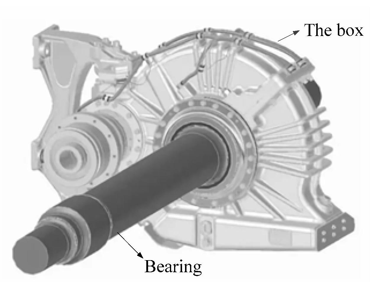
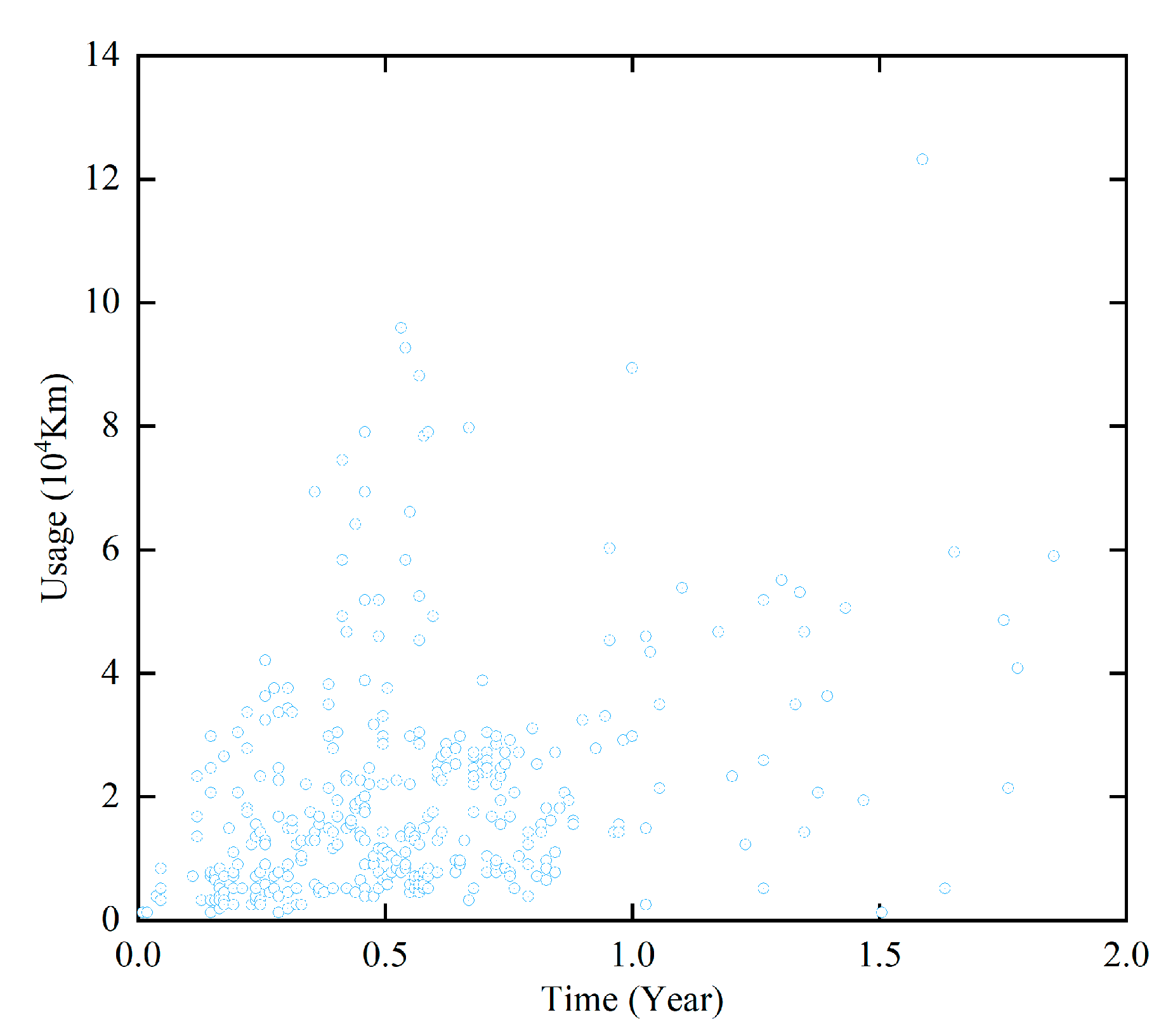
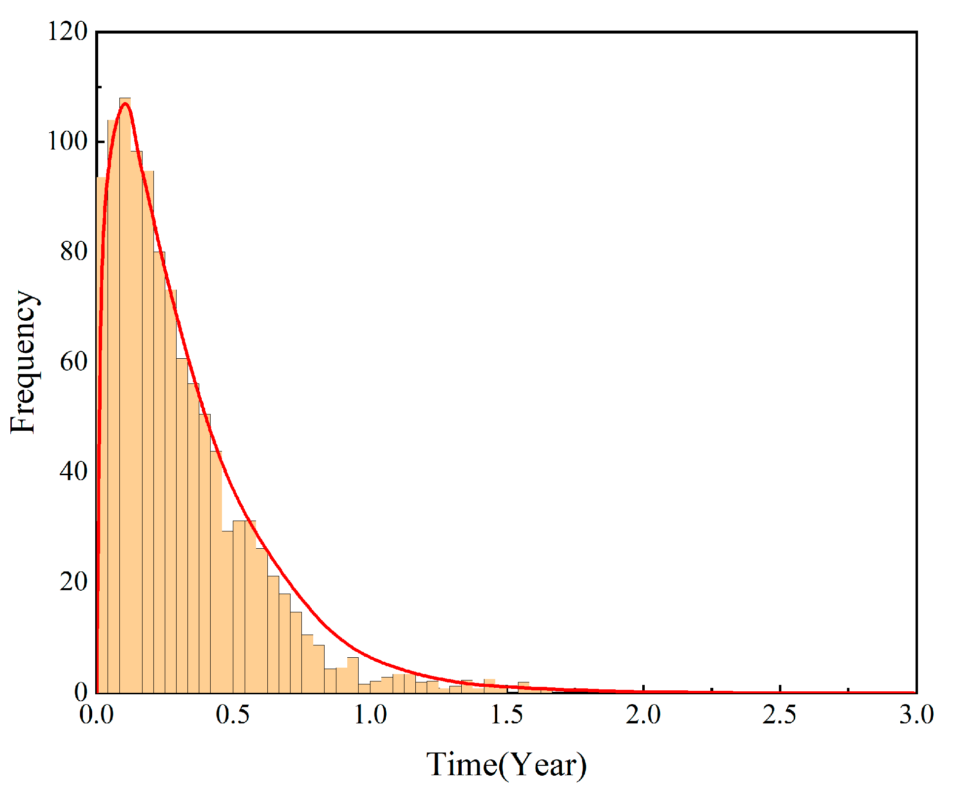
5.1. Problem Description

As a complex electromechanical system, an EMU system is composed of many multi-component systems. There are functional and mechanical high-strength couplings and high-density connections between the components, which makes it possible for failure dependence. Taking a gearbox as an example, the failure of the bearing will enhance the failure rate and aggravate the failure of the gear, as shown in Figure 5. In the gearbox, the bearing can be regarded as the key component, and the gear can be regarded as the subsystem. There is failure dependence between the bearing and the gear. The manufacturer offers a 2D EW for the gearbox. The formulation of the 2D EW contract of the gearbox should meet the availability requirements and ensure the lowest EW cost for the manufacturer.
Since the gearbox has a low rate of failure within the duration of a basic warranty, only the post-failure minimum maintenance can be considered. During the EW period, the gearbox has been in service for a period of time, and the failure rate increases significantly. Based on the minimum maintenance after failure, it is necessary to conduct imperfect preventive maintenance. Through field investigation, we collected the failure history data of the CRH6-200 gearbox, which is widely used in EMU systems in China. The data included the time to first failure (year) and the kilometer at the failure time for the bearing. We collected a total of 1000 groups of data and plotted a scatter diagram, as shown in Figure 6.
The designed utilization rate r s of this gearbox is 1 × 10 4   KM / y e a r . We plotted a histogram of bearing failure time as shown in Figure 7. As can be seen from Figure 7, when compared to the utilization rate, the time to the first failure of the bearing was subject to Weibull distribution, with the scale parameter α s = 0.7 and the shape parameter φ = 1.1 .
F 0 ( t ; α s ) = 1 exp [ ( t / α s ) φ ] = 1 exp [ ( t / 0.7 ) 1.1 ]
For the rate of utilization r , the cumulative distribution function for bearing failure is:
F ( t ; α r , φ ) = F s ( t ; α s ( r s r ) γ , φ ) = 1 exp [ ( r r s ) γ φ t φ α s φ ]
In accordance with the AFT model presented in Section 3.1, the failure rate function of the bearing is:
λ ψ ( t ; r ) = f ( t ; α r ) F ¯ ( t ; α r ) = φ ( r r s ) γ φ t φ 1 α s φ
where the AFT parameter γ = 1.2 .
We learned from the manufacturer that the gearbox utilization rate conforms to a uniform distribution on ( 0.1 , 10 ) :
r ~ U ( 0.1 , 10 )
That is:
g ( r ) = 10 99 ( 0.1 < r < 10 )
It is known that the gearbox has a 2D basic warranty period with W = 2   y e a r s and U = 2 × 10 4   KM . The gear failure rate is λ s = 4 × 10 4 / d a y . The minimum maintenance time of the bearing is T f 1 = 7   d a y s , and the minimum maintenance cost is CNY 1500. The minimum maintenance time of the gear is T f 2 = 12   d a y s , and the minimum maintenance cost is CYN 2000. The time for preventive maintenance of the gearbox is T p = 4   d a y s , and the cost of preventive maintenance is CNY 600. The imperfect preventive maintenance improvement factor is δ = 0.6 . The maintenance experience and data analysis indicate that a bearing failure will increase the gear failure rate, and the failure influence coefficient is θ = 0.5 . The availability of the gearbox should not be less than 0.6 in each replacement cycle (EW period). By solving the optimal interval of preventive maintenance and cycle of replacement, the minimum warranty cost per unit time of the gearbox in the replacement cycle can be obtained with the availability meeting the requirements.

5.2. Model Solution

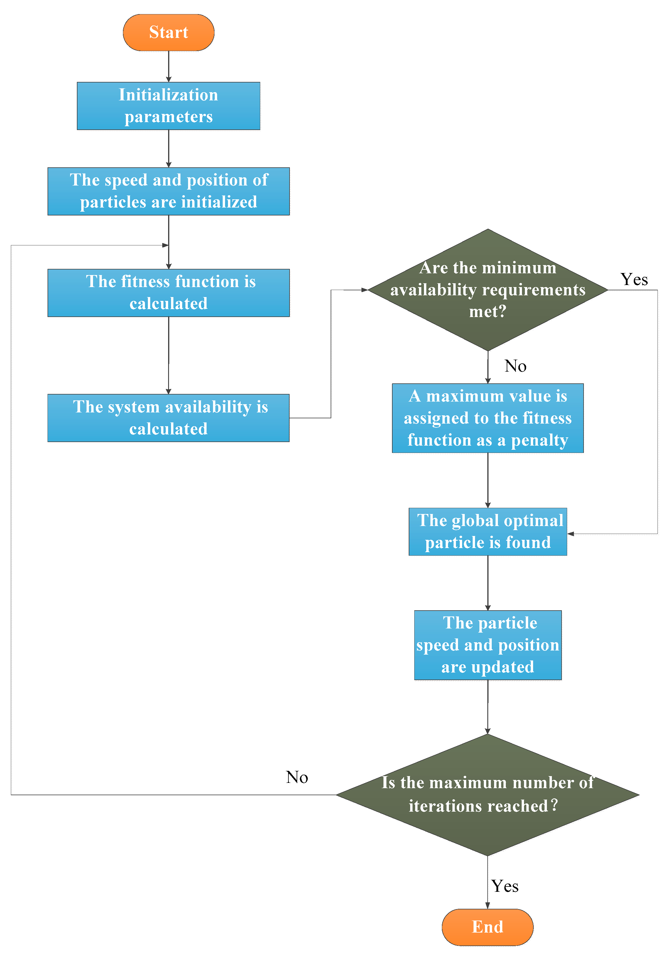
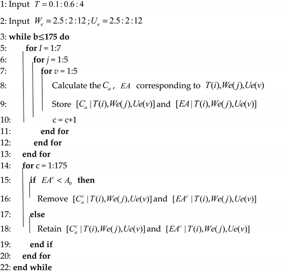
5.2.1. The Grid Search Method

Firstly, the grid search method was adopted for solving the model. This method is also called the enumeration method, and its principle is relatively simple. By setting the value range and changing the steps of decision variables, all possible combinations of the decision variables can be obtained, and each combination represents a scheme. Firstly, whether the combination of the decision variables meets the constraints is judged, and then combinations that meet the constraints are bought into the objective function in turn. By comparing the value of the objective function, the optimal scheme is obtained. Considering the actual situation, the value of the preventive maintenance interval T of the gearbox was [ 0.1   y e a r s ,   4   y e a r s ] , and the change step was 0.6 years. The value range of the EW period W e was [ 2.5   y e a r s ,   12   y e a r s ] , and the change step was 2 years. The value range of the EW period U e was [ 2.5 × 10 4   KM , 12 × 10 4   KM ] , and the change step was 2 × 10 4   KM . The replacement cost of the gearbox was CNY 36,000. The models of the 2D EW cost per unit of time and availability were simulated by employing the grid search method, based on which changes in the warranty cost per unit time and the availability were derived within the EW periods W e , U e , and T . The algorithm’s basic steps are presented in Table 2.
The grid search method was executed for 175 iterations. The results show that when We = 8.5 years, Ue = 6.5 × 10⁴ KM, and T = 0.1 years, the warranty cost per unit time within the EW period was the lowest, which was 128,708 CNY/year, and the availability was 0.8584.

5.2.2. The PSO–BAS Algorithm

Three variables were involved in this example, and the solving process of the grid search method had low efficiency and poor accuracy. This paper used the PSO–BAS algorithm to enhance the grid search method. Particle swarm optimization (PSO) is a group collaboration-based algorithm that is created through the mimicry of avian foraging. At its core, PSO attempts to allow the disorder-to-order evolution of the entire swarm in the problem-solving space by exploiting the inter-swarm individual sharing of information. The key formula of the algorithm is:
v i d = w v i d - 1 + c 1 r 1 ( p b e s t i d x i d ) + c 2 r 2 ( g b e s t i d x i d )
where v i d represents the velocity of particle i in step d; w represents the inertia weight; c 1 and c 2 represent the learning factor; r 1 and r 2 are usually random numbers within [0, 1]; x i d represents the position of particle i in step d; and p b   e s t i d and g b   e s t i d stand for the best position of the individual and group, separately. According to the formula, the speed of the particle in step d was affected not only by its own speed inertia, but also by self-cognition and social cognition. This mechanism promoted the algorithm with the purpose of finding the global optimal solution in the set of feasible solutions.
Then, the position of the particle in step d + 1 is:
x i d + 1 = x i d + v i d
As a meta-heuristic algorithm following the foraging principles of longicorn beetles, the fundamentals of the beetle antennae search (BAS) algorithm is that longicorn beetles determine the next direction by judging the odor intensity received by their two antennae. Through combining the PSO algorithm with the BAS algorithm (i.e., PSO–BAS) and treating each particle as a longicorn beetle, the longicorn beetle particles will turn before each position update, which can efficiently improve the algorithmic searching capacity both globally and locally. In the iterative process, the fitness function value of the left antenna is compared with that of the right antenna, and the better one is used to update the direction of the longicorn beetles, thereby improving the global searching capacity and preventing the algorithm from falling into local optima.
The specific steps of the PSO–BAS algorithm are:
Step 1: Population initialization is performed. The position x i d and speed v i d of the longicorn particle are set in step d. The maximum speed is v m a x , and the minimum speed is v m i n ; the distance between the two antennae of the longicorn beetle is q, and the maximum number of iterations is K.
Step 2: For every longicorn particle, its corresponding value of fitness is calculated, and p b   e s t i d and g b   e s t i d of the longicorn particles are updated.
Step 3: The longicorn particle speed v i d + 1 is updated according to Equation (37).
Step 4: Taking the position of the current particle as the centroid of the longicorn, the orientation of the individual longicorn is generated randomly:
b = r a n d s ( k ^ , 1 ) | r a n d s ( k ^ , 1 ) |
where k ^ is the spatial dimension and r a n d s ( ) is the random function. In this case, k ^ was 3.
Step 4: To determine the position of the left and right antennae of longicorn particles, the calculation formula is:
x i l d = x i d b u d / 2
x i r d = x i d + b u d / 2
where, x i l d and x i r d are respectively the position of the left antenna and the right antenna of the longicorn particle. The term u d represents the distance between the left and right antennae of the longicorn beetle in the d iteration. If u d is larger, the longicorn particle can search in a larger range, and u d usually becomes smaller and smaller as the iteration progresses. The u d is given by Jiang [4] as u d = 0.95 u d 1 + 0.01 and u 1 = 2 . The linear decreasing weight strategy was adopted to set the step factor ϑ to ensure that the longicorn particles could include the current search area and avoid the algorithm from falling into local minima, i.e., ϑ = ϑ d e a t , d = ( 0 , 1 , , K ) , e a t ( 0 , 1 ) . The fit( x i l d ) and fit( x i r d ) terms respectively represent the odor concentration to be received by the left antenna and right antenna, where fit ( · ) is the fitness function. The perceived speed of a longicorn antennae is:
ξ i d + 1 = ϑ d b s i g n [ f i t ( x i r d ) f i t ( x i l d ) ]
where s i g n ( ) is a symbolic function, and its definition formula is:
s i g n ( x ) = { 1   x > 0 Keep   the   current   direction   x = 0 1 otherwise
The location-updating formula of the longicorn particles is as follows:
x i d + 1 = x i d + v i d + 1 + ( 1 ) ξ i d + 1
where is the speed weight, and its value is between 0 and 1.
In this case, We, Ue, and T were taken as longicorn particles, the EW cost per unit time was taken as the fitness function, and the constraints of the availability were considered. For this case, the flow chart for applying the PSO–BAS algorithm is shown in Figure 8.
The fundamental algorithmic procedure is presented in Table 3.
The initial values of the algorithm parameters are presented in Table 4.
To show the advantages of the PSO–BAS algorithm, the PSO algorithm and PSO–BAS algorithm were respectively used to solve the optimal EW scheme of the gearbox system. Similar to the grid search algorithm, the PSO algorithm and PSO–BAS algorithm underwent 175 iterations. Figure 9 depicts the lowest 2D EW cost per unit time found by the two algorithms with increasing iterations.
In accordance with Figure 9, as the PSO–BAS algorithm iterates, the 2D EW cost per unit time of the gearbox continued to decrease. When the algorithm reached the 35th iteration, the optimal value of 126,305 CNY/year was found, and the optimal value remained stable until the end of the iteration. The optimal 2D EW period corresponding to this value was (8.4years, 7.2 × 10⁴ KM) with the optimal preventive maintenance interval T being 0.3 years.
For the PSO algorithm, when it reached the 20th iteration, the optimal value of 127,812 CNY/year was found, and the optimal value remained stable until the end of the iteration. The optimal 2D EW period corresponding to this value was (8.4 years, 6.9 × 10⁴ KM), and the optimal interval of preventive maintenance T was 0.1 years. A comparison between the grid search method, the PSO algorithm, and the PSO–BAS algorithm is presented in Table 5.
It can be found from Table 6 that the EW scheme with a lower EW cost per unit time and a higher system availability can be obtained through the PSO–BAS algorithm with improved operational efficiency. In addition, it can be seen from Figure 9 and Table 6 that although the PSO algorithm converges quickly, it easily falls into the local optima. The PSO–BAS algorithm effectively improves the global search capability of the PSO algorithm and stops it from falling into the local optima.

5.3. Result Analysis

5.3.1. Dimension Reduction Analysis

We was fixed to 8.5 years, and Ue was fixed to 10.5 × 10⁴ KM. Then, the variation in the EW cost per unit time and system availability with the preventive maintenance interval T was obtained.
It can be seen from Figure 10 that with an increase in T, the EW cost decreased first and subsequently increased, and the availability increased first and subsequently reduced. Meanwhile, there was an optimal T that made the EW cost per unit time the lowest or the availability the highest.
Next, T was fixed to 0.1 years, and the change in the EW’s cost per unit time and the system availability with the EW period was obtained.
According to Figure 11, when the preventive maintenance interval was fixed, there was an optimal EW period that minimized the EW cost per unit time or maximized the system availability.
Through the analysis in Section 4.2, the optimal preventive maintenance interval under different 2D EW periods could be obtained, as shown in Table 6.
The EW cost per unit time and the system availability under different EW schemes are presented in Table 7 and Table 8, separately.
In practical applications, the optimal warranty cost per unit time and the system availability under different EW periods can be estimated, which provides a scientific basis for formulating the warranty strategy.

5.3.2. Comparative Analysis
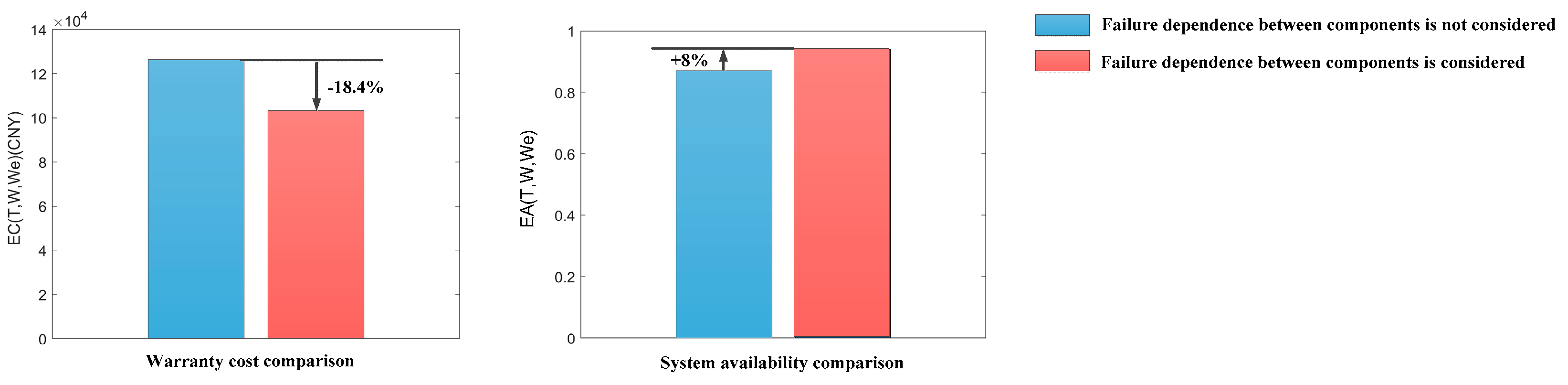
(1)
According to the analysis in Section 4.2, the 2D EW period was (8.4 years, 7.2 × 10⁴ KM), and the preventive maintenance interval was 0.3 years. To verify the impact of imperfect preventive maintenance on reducing the EW cost and improving system availability, this paper compared the EW cost and the system availability of the gearbox system when only adopting corrective maintenance, and the gearbox system when adopting both corrective maintenance and imperfect preventive maintenance. When the system did not carry out preventive (imperfect) maintenance within the EW duration, i.e., the preventive maintenance interval was set to 8.4 years, the corresponding EW cost per unit time and the system availability were as follows:
W e = 8.4   y e a r s ,   U e = 7.2 × 10 4   KM ,   T = 8.4   y e a r s ,   EC = 244312 CNY / year ,   EA = 0.52
When the 2D EW period was (8.4 years, 7.2 × 10⁴ KM), the strategy formulated in this paper was to adopt both corrective and preventive maintenance during the EW duration, with the optimal anticipated interval of preventive maintenance being 0.3 years. Meanwhile, the warranty cost per unit time and the system availability during the EW period were as follows:
W e = 8.4   y e a r s ,   U e = 7.2 × 10 4   KM ,   T = 0.3   y e a r s ,   EC = 126305 CNY / year ,   EA = 0.87
As shown in Figure 12, after adopting the imperfect preventive maintenance strategy, the EW cost per unit time was reduced by 48%, and the system availability was increased by 67%, thus attaining a win-win between the manufacturers and the users.
(2)
This paper considered the failure dependence between the bearing and the gear. If the failure dependence between the components was ignored, assuming that θ = 0 , the EW period and the preventive maintenance interval that minimized the EW cost per unit time could be calculated according to the model. The EW cost per unit time and the system availability under this scheme were as follows:
W e = 10.5   y e a r s ,   U e = 8.5 × 10 4   KM ,   T = 1.7   y e a r s ,   EC = 103124 CNY / year ,   EA = 0.94
As shown in Figure 13, when assuming that there was no failure dependence between components, the optimal EW period and the preventive maintenance interval were longer, the corresponding EW cost per unit time was lower, and the system availability was higher. Although the results seem to be better, the assumption of independent failure was unrealistic, so the calculation results were inconsistent with the actual situation. It also proved that ignoring failure dependence will lead to unacceptable analysis errors and decision errors, which will unrealistically lower the manufacturer’s anticipation of the cost and elevate the user’s expectations of system availability.

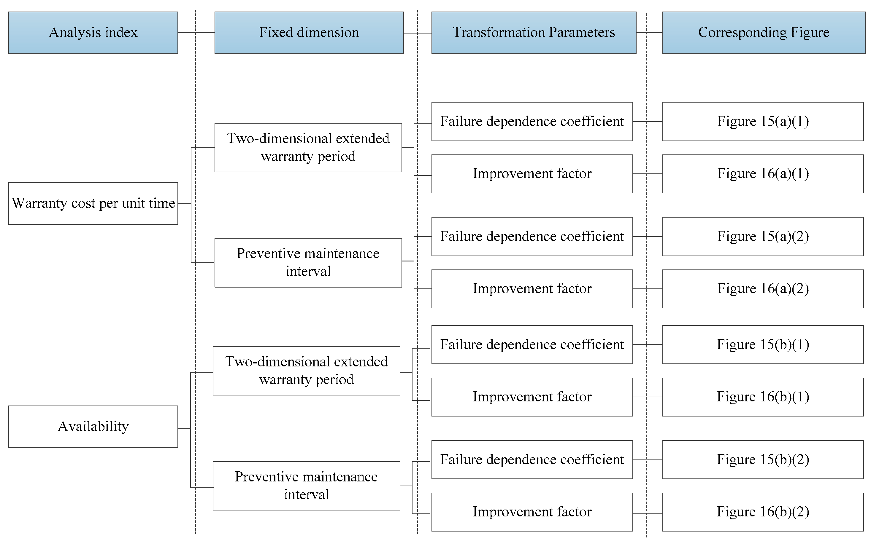
5.4. Sensitivity Analysis
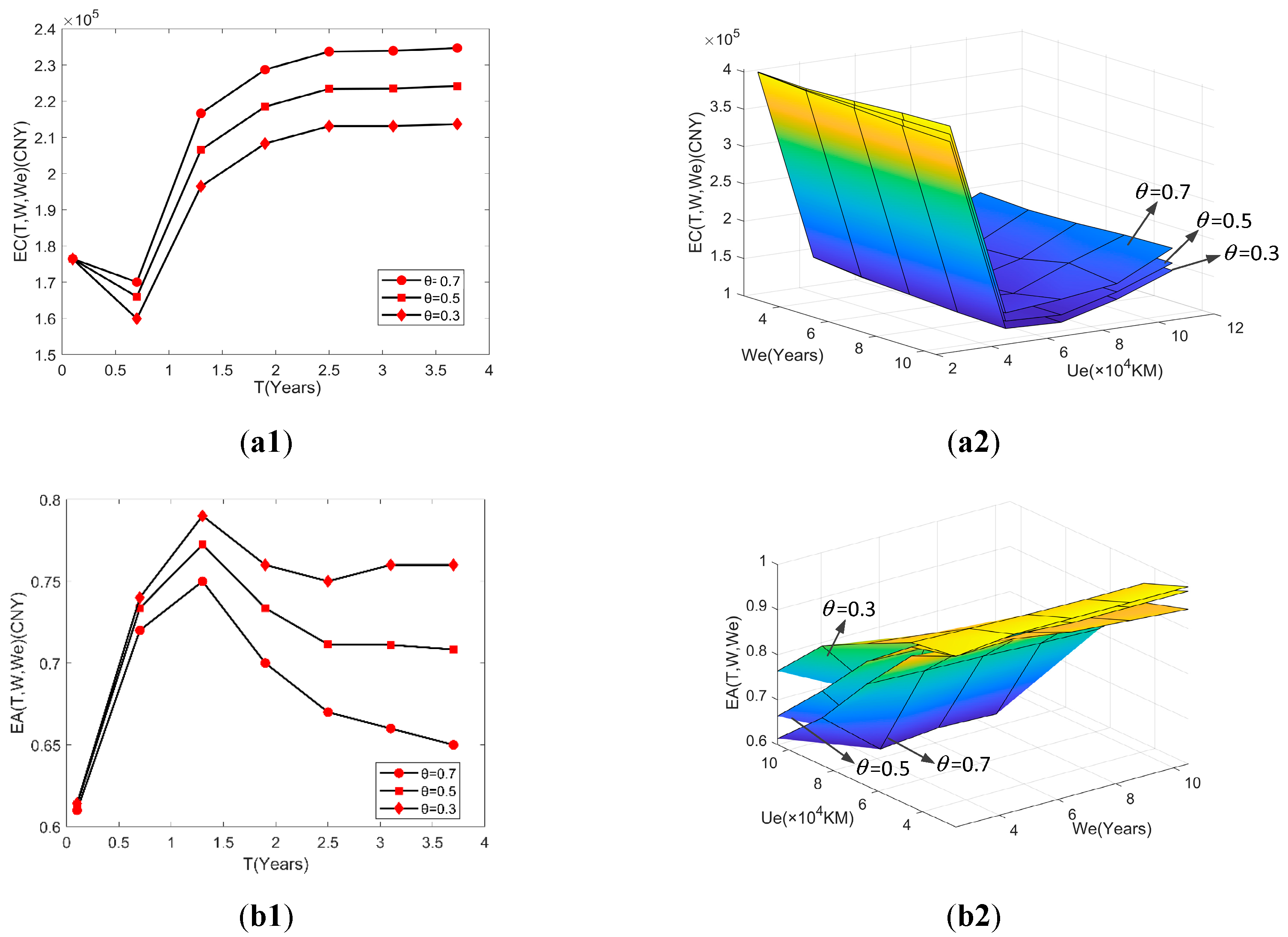
In the model established in the current work, the failure-dependence coefficient θ and the imperfect preventive maintenance improvement factor δ will have a certain impact on the EW cost per unit time and the gearbox availability. To investigate the impact, a sensitivity analysis was carried out for θ and δ , and the variation trend of the EW cost per unit time and the availability for the gearbox are shown. The analysis of this part is shown in Figure 14.

5.4.1. Failure-Dependence Coefficient θ Impact Analysis

We was fixed to 8.5 years, Ue was fixed to 10.5 × 10⁴ KM, and θ was changed. The change in the EW cost per unit time and the availability of the gearbox with T under different θ are shown in Figure 15(a1,b1), respectively. Next, T was fixed to 0.1 years, and θ was changed. The change in the EW cost per unit time and the availability of the gearbox with (We,Ue) under different θ are shown in Figure 15(a2,b2), respectively.
As shown in Figure 15, the larger θ was, the higher the EW cost of the gearbox and the lower the availability. This was mainly because the larger θ was, the greater the impact of the bearing on the failure of the gear was, and the higher the expected minimum maintenance times of the gear were. This contributed to the enhancement of the warranty cost of the gearbox and the decrease in availability.
Meanwhile, with an increase in the preventive maintenance interval and the EW period, the difference in the gearbox EW cost or system availability under different θ increased. This was mostly due to the fact that longer preventive maintenance intervals or EW periods corresponded with an increase in the expected failure times of the bearing, an increase in the actual failure rate of the gear, an increase in the expected minimum maintenance times, a higher EW cost for the gearbox, and a lower availability. Since the failure-dependence coefficient is determined in the design stage of a system, manufacturers should focus on the failure dependence between components and strive to reduce the failure-dependence coefficient. Only in this way can the warranty cost of the system be reduced and the system availability be improved during the warranty period.

5.4.2. Improvement Factor δ Impact Analysis

We was fixed to 8.5 years, and Ue was fixed to 10.5 × 10⁴ KM. Then, the change in the EW cost per unit time and the availability of the gearbox system with T under different δ values are shown in Figure 16(a1,b1), respectively. Next, T was fixed to 0.1 years, and the change in the EW cost per unit time and availability of the gearbox system with (We,Ue) under different δ values are shown in Figure 16(a2,b2), respectively.
It can be seen from Figure 16 that the larger δ was, the lower the cost of the gearbox EW cost, and the higher the availability. This was mostly due to the fact that larger δ values corresponded with better effects of imperfect preventive maintenance on reducing the system failure rate and a lower expected minimum maintenance times of the gear. This increased the availability of the gearbox system and decreased the warranty cost. The imperfect preventive maintenance improvement factor δ generally reflects the maintenance level of the manufacturer. Thus, the manufacturer can pursue a higher improvement coefficient δ for preventive (imperfect) maintenance by improving the quality of maintenance workers, improving the maintenance technology, and strengthening technological innovation.

6. Conclusions

Based on a multi-component failure-dependence analysis, this paper comprehensively considered preventive maintenance and corrective maintenance, and established a two-dimensional extended warranty cost model per unit time and an availability model for the multi-component system by using imperfect preventive maintenance theory and non-homogeneous Poisson process theory. By taking the lowest warranty cost per unit time as the goal and the availability as the constraint, a two-dimensional extended warranty decision-making model was established. In the case analysis, a grid search algorithm, PSO algorithm, and PSO–BAS algorithm were used to obtain the optimal two-dimensional extended warranty scheme for the gearbox of an EMU system. It was found that using a PSO–BAS algorithm could obtain a two-dimensional extended warranty scheme with a lower warranty cost and a higher availability. Through comparative analysis, the necessity of imperfect preventive maintenance during the two-dimensional extended warranty period was verified. In the case of imperfect preventive maintenance, the cost of a two-dimensional extended warranty per unit time was reduced by 48%, while the availability was increased by 67%. In addition, it was also verified that ignoring failure dependence will lead to unacceptable analysis errors. The analysis results showed that the model established in this paper has good practicability and effectiveness, and could provide a quantitative analysis method for the two-dimensional extended warranty decision making of a failure-dependence system. A manufacturer could use the model proposed in this paper to obtain a two-dimensional extended warranty scheme that could enable a win-win situation for the buyer and the seller of the failure-dependence multi-component system. The sensitivity analysis results showed that in the design stage, manufacturers should pay attention to the failure dependence between components and strive to reduce the failure-dependence coefficient. In addition, manufacturers should pursue higher imperfect preventive maintenance improvement factors. The following meaningful directions can be considered for future research:
(1)
More complex failure dependencies between system components should be considered, such as common cause failure, interactive failure, and retained redundancy.
(2)
The failure dependence and economic dependence among multiple components should be considered comprehensively to make warranty decisions.
(3)
Considering market factors, the joint decision making of two-dimensional extended warranty schemes and pricing should be carried out.

Author Contributions

Conceptualization, E.D. and Z.C.; methodology, R.W.; software, E.D.; validation, E.D. and R.W.; writing—original draft preparation, E.D.; writing—review and editing, Z.C. and R.W.; visualization, E.D.; supervision, J.Z.; project administration, Z.C.; funding acquisition, Z.C. All authors have read and agreed to the published version of the manuscript.

Funding

The present study was funded by the National Natural Science Foundation of China (no. 71871219).

Institutional Review Board Statement

Not applicable.

Informed Consent Statement

Not applicable.

Data Availability Statement

All data generated or explored during this study are covered in this work.

Acknowledgments

Not applicable.

Conflicts of Interest

The authors declare no conflict of interest.

Nomenclature

Variables
W Basic warranty period of time dimension under design utilization
U Basic warranty period of usage dimension under design utilization
W e Extended warranty period of time dimension under design utilization
U e Extended warranty period of usage dimension under design utilization
T The interval of preventive (imperfect) maintenance
t The calendar time
r Component of system utilization
T s The time of the first failure based on the design rate of utilization r s
T r The time of the first failure based on the real rate of utilization   r
δ Imperfect preventive maintenance improvement factor
θ Failure-dependence coefficient
α r Scale parameter of the failure probability density function
γ The AFT parameter
m k ψ Failure times of the key component within the interval of the kth preventive maintenance
Functions
W Θ ( r ) The start time of the EW period for the utilization rate r
g ( r ) Probability density function of utilization r
E C ( T , a , b ) Two-dimensional extended warranty cost in (a, b)
λ k ψ ( t | r ) The key component failure rate within the in-terval of the kth preventive maintenance for the utilization rate r
λ k s ( t | r ) The subsystem failure rate within the interval of the kth preventive maintenance for the utilization rate r
f ( t ; α r ) Failure probability density function for the utili-zation rate r
F ¯ ( t ; α r ) Reliability function for the utilization rate r
W Φ ( r ) The end time of the EW period for the utilization rate r
λ a ( t | r ) The real failure rate of the component a for the utilization rate r

References

  1. Huang, Y.S.; Fang, C.C.; Lu, C.M.; Tseng, T.L.B. Optimal Warranty Policy for Consumer Electronics with Dependent Competing Failure Processes. Reliab. Eng. Syst. Saf. 2022, 222, 108418. [Google Scholar] [CrossRef]
  2. Huang, Y.S.; Huang, C.D.; Ho, J.W. A customized two-dimensional extended warranty with preventive maintenance. Eur. J. Oper. Res. 2017, 257, 525–535. [Google Scholar] [CrossRef]
  3. Mitra, A. Warranty parameters for extended two-dimensional warranties incorporating consumer preferences. Eur. J. Oper. Res. 2021, 219, 971–978. [Google Scholar] [CrossRef]
  4. Dong, E.; Cheng, Z.; Wang, R. Two-Dimensional Extended Warranty Strategy for an Economic Dependence Multi-Component Series System with Grid Search Algorithm. IEEE Access 2022, 10, 26876–26894. [Google Scholar] [CrossRef]
  5. Abeygunawardane, S.K.; Jirutitijaroen, P. Application of Probabilistic Maintenance Models for Selecting Optimal Inspection Rates Considering Reliability and Cost Tradeoff. IEEE Trans. Power Deliv. 2014, 29, 178–186. [Google Scholar] [CrossRef]
  6. Wang, J.X.; Lin, B.L.; Jin, J.C. Optimizing the Shunting Schedule of Electric Multiple Units Depot Using an Enhanced Particle Swarm Optimization Algorithm. Comput. Intell. Neurosci. 2016, 2016, 5804626. [Google Scholar] [CrossRef] [PubMed] [Green Version]
  7. Mao, B.; Xie, Z.; Wang, Y.; Handroos, H.; Wu, H.; Shi, S. A hybrid differential evolution and particle swarm optimization algorithm for numerical kinematics solution of remote maintenance manipulators. Fusion Eng. Des. 2017, 124, 587–590. [Google Scholar] [CrossRef]
  8. Pereira, C.M.; Lapa, C.M.; Mol, A.C.; Da Luz, A.F. A Particle Swarm Optimization (PSO) approach for non-periodic preventive maintenance scheduling programming. Prog. Nucl. Energy 2010, 52, 710–714. [Google Scholar] [CrossRef]
  9. Jiang, X.Y.; Li, S. BAS: Beetle Antennae Search Algorithm for Optimization Problems. Int. J. Robot. Control. 2017, 1, 10724. [Google Scholar] [CrossRef]
  10. Wang, X.; Xie, W. Two-dimensional warranty: A literature review. Proc. Inst. Mech. Eng. Part O J. Risk Reliab. 2017, 232, 284–307. [Google Scholar] [CrossRef]
  11. Iskandar, B.P.; Murthy, D.N.P.; Jack, N. A new repair–replace strategy for items sold with a two-dimensional warranty. Comput. Oper. Res. 2005, 32, 669–682. [Google Scholar] [CrossRef]
  12. Cheng, Z.H.; Yang, Z.Y.; Zhao, J.M.; Wang, Y.B.; Li, Z.W. Preventive maintenance strategy optimizing model under twodimensional warranty policy. Eksploat. Niezawodn. 2015, 17, 365–373. [Google Scholar] [CrossRef]
  13. Cheng, Z.H.; Yang, Z.Y.; Yang, H.B. Optimization model of equipment two-dimensional warranty strategy under preventive maintenance. Ind. Eng. J. 2017, 20, 79–86. [Google Scholar]
  14. Chen, T.; Popova, E. Maintenance policies with two-dimensional warranty. Reliab. Eng. Syst. Saf. 2002, 77, 61–69. [Google Scholar] [CrossRef]
  15. Jack, N.; Murthy, D.N.P.; Iskandar, B.P. Comments on “Maintenance policies with two-dimensional warranty”. Reliab. Eng. Syst. Saf. 2003, 82, 105–109. [Google Scholar] [CrossRef]
  16. Su, C.; Wang, X. Optimal upgrade policy for used products sold with two-dimensional warranty. Qual. Reliab. Eng. Int. 2016, 32, 2889–2899. [Google Scholar] [CrossRef]
  17. Varnosafaderani, S.; Chukova, S. A two-dimensional warranty servicing strategy based on reduction in product failure intensity. Comput. Math. Appl. 2012, 63, 201–213. [Google Scholar] [CrossRef] [Green Version]
  18. Peng, S.; Jiang, W.; Zhao, W. A preventive maintenance policy with usage-dependent failure rate thresholds under two-dimensional warranties. Iise Trans. 2021, 53, 1231–1243. [Google Scholar] [CrossRef]
  19. Baik, J.; Murthy, D.N.P.; Jack, N. Two-dimensional failure modeling with minimal repair. Nav. Res. Logist. 2003, 51, 345–362. [Google Scholar] [CrossRef]
  20. Wang, X.; Li, L.; Xie, M. An unpunctual preventive maintenance policy under two-dimensional warranty. Eur. J. Oper. Res. 2020, 282, 304–318. [Google Scholar] [CrossRef]
  21. Zheng, R.; Su, C. A flexible two-dimensional basic warranty policy with two continuous warranty regions. Qual. Reliab. Eng. Int. 2020, 36, 2003–2018. [Google Scholar] [CrossRef]
  22. He, Z.; Wang, D.; He, S.; Zhang, Y.; Dai, A. Two-dimensional extended warranty strategy including maintenance level and purchase time: A win-win perspective. Comput. Ind. Eng. 2020, 141, 106294. [Google Scholar] [CrossRef]
  23. Wang, Q.; Cheng, Z.; Gan, Q.; Bai, Y.; Zhang, J. Cost Optimization of Two-Dimensional Warranty Products under Preventive Maintenance. Math. Probl. Eng. 2021, 2021, 2538050. [Google Scholar] [CrossRef]
  24. Wang, R.; Cheng, Z.; Wang, Q. Research on Availability Model of Two-dimensional Warranty Products Based on Incomplete Maintenance. IOP Conf. Ser. Mater. Sci. Eng. 2021, 1043, 032046. [Google Scholar] [CrossRef]
  25. Zhu, H.H. Two Dimensional Warranty Modeling and Optimization Based on Preventive Maintenance; Shijiazhuang Railway University: Shaoxing, China, 2020. [Google Scholar]
  26. Dai, A.; Zhang, Z.; Hou, P.; Yue, J.; He, S.; He, Z. Warranty Claims Forecasting for New Products Sold with a Two-Dimensional Warranty. J. Syst. Sci. Syst. Eng. 2019, 28, 715–730. [Google Scholar] [CrossRef]
  27. Peng, T.; Chunling, L. Designing differential service strategy for two-dimensional warranty based on warranty claim data under consumer-side modularisation. Proc. Inst. Mech. Eng. Part O J. Risk Reliab. 2019, 234, 550–561. [Google Scholar] [CrossRef]
  28. Lin, K.; Chen, Y. Analysis of two-dimensional warranty data considering global and local dependence of heterogeneous marginals. Reliab. Eng. Syst. Saf. 2021, 207, 107327. [Google Scholar] [CrossRef]
  29. Tong, P.; Song, X.; Zixian, L. A maintenance strategy for two-dimensional extended warranty based on dynamic usage rate. Int. J. Prod. Res. 2017, 55, 5743–5759. [Google Scholar] [CrossRef]
  30. Wang, D.; He, Z.; He, S.; Zhang, Z.; Zhang, Y. Dynamic pricing of two-dimensional extended warranty considering the impacts of product price fluctuations and repair learning. Reliab. Eng. Syst. Saf. 2021, 210, 107516. [Google Scholar] [CrossRef]
  31. Wang, X.; Ye, Z.-S. Design of customized two-dimensional extended warranties considering use rate and heterogeneity. IISE Trans. 2020, 53, 341–351. [Google Scholar] [CrossRef]
  32. Yang, G.E.; Gao, Q.; Huang, Z.X. Maintenance Interval Period Optimization Method of Complex System Based on Availability. Fire Control. Command. Control. 2013. [Google Scholar]
  33. Pariaman, H.; Garniwa, I.; Surjandari, I.; Sugiarto, B. Availability Analysis of the Integrated Maintenance Technique based on Reliability, Risk, and Condition in Power Plants. Int. J. Technol. 2017, 8, 497. [Google Scholar] [CrossRef]
  34. Qiu, Q.; Liu, B.; Lin, C.; Wang, J. Availability analysis and maintenance optimization for multiple failure mode systems considering imperfect repair. Proc. Inst. Mech. Eng. Part O J. Risk Reliab. 2021, 235, 982–997. [Google Scholar] [CrossRef]
  35. Ahn, S.; Kim, W. On determination of the preventive maintenance interval guaranteeing system availability under a periodic maintenance policy. Struct. Infrastruct. Eng. 2011, 7, 307–314. [Google Scholar] [CrossRef]
  36. Wang, R.; Cheng, Z.; Rong, L.; Bai, Y.; Wang, Q. Availability Optimization of Two-dimensional Warranty Products Under Imperfect Preventive Maintenance. IEEE Access 2021, 9, 8099–8109. [Google Scholar] [CrossRef]
  37. Dong, E.; Cheng, Z.; Wang, R.; Zhang, X. Availability Optimization of Multicomponent Products with Economic Dependence under Two-Dimensional Warranty. Discret. Dyn. Nat. Soc. 2021, 2021, 2492430. [Google Scholar] [CrossRef]
  38. Su, C.; Cheng, L. Two-dimensional preventive maintenance optimum for equipment sold with availability-based warranty. Proc. Inst. Mech. Eng. Part O J. Risk Reliab. 2019, 233, 648–657. [Google Scholar] [CrossRef]
  39. Peng, W.; Zhang, X.; Huang, H. A failure rate interaction model for two-component systems—Based on copula function with shock damage interaction. J. Risk Reliab. 2016, 230, 278–284. [Google Scholar]
  40. Sun, Y. Reliability Prediction of Complex Repairable Systems: An Engineering Approach; Queensland University of Technology: Brisbane, Australia, 2006. [Google Scholar]
  41. Sun, Y.; Ma, L.; Mathew, J.; Zhang, S. An analytical model for interactive failures. Reliab. Eng. Syst. Saf. 2006, 91, 495–504. [Google Scholar] [CrossRef]
  42. Zhang, N.; Fouladirad, M.; Barros, A.; Zhang, J. Condition-based maintenance for a K-out-of-N deteriorating system under periodic inspection with failure dependence. Eur. J. Oper. Res. 2020, 287, 159–167. [Google Scholar] [CrossRef]
  43. Dong, E.; Cheng, Z.; Wang, R.; Zhang, Y. Extended warranty decision model of failure dependence wind turbine system based on cost-effectiveness analysis. Open Phys. 2022, 20, 616–631. [Google Scholar] [CrossRef]
  44. Qian, Q.; Jiang, Z.H. Preventive maintenance strategy and maintenance time of multi-component system. Ind. Eng. 2020, 23, 95–100. [Google Scholar]
  45. Wang, H.; Du, W.; Liu, Z.; Yang, X.; Li, Z. Multi component system maintenance of EMU based on joint fault and economic correlation. J. Shanghai Jiaotong Univ. 2016, 50, 660–667. [Google Scholar]
  46. Keizer MC, O.; Flapper SD, P.; Teunter, R.H. Condition-based maintenance policies for systems with multiple dependent components: A review. Eur. J. Oper. Res. 2017, 261, 405–420. [Google Scholar] [CrossRef]
  47. Lawless, J.; Hu, J.; Cao, J. Methods for the estimation of failure distributions and rates from automobile warranty data. Lifetime Data Anal. 1995, 1, 227–240. [Google Scholar] [CrossRef] [PubMed]
  48. Tong, P.; Liu, Z.; Men, F.; Cao, L. Designing and pricing of two-dimensional extended warranty contracts based on usage rate. Int. J. Prod. Res. 2014, 52, 6362–6380. [Google Scholar] [CrossRef]
  49. Zhao, X.; Xie, M. Using accelerated life tests data to predict warranty cost under imperfect repair. Comput. Ind. Eng. 2017, 107, 223–234. [Google Scholar] [CrossRef]
  50. Pham, H.; Wang, H. Imperfect maintenance. Eur. J. Oper. Res. 1996, 94, 425–438. [Google Scholar] [CrossRef]
  51. Shaomin, W.; Zuo, M.J. Linear and Nonlinear Preventive Maintenance Models. IEEE Trans. Reliab. 2010, 59, 242–249. [Google Scholar] [CrossRef] [Green Version]
  52. Wang, Y.; Liu, Z.; Liu, Y. Optimal preventive maintenance strategy for repairable items under two-dimensional warranty. Reliab. Eng. Syst. Saf. 2015, 142, 326–333. [Google Scholar] [CrossRef]
Figure 1. Unidirectional failure-dependence model.
Processes 10 01479 g001
Figure 2. Schematic diagram of the virtual age method.
Processes 10 01479 g002
Figure 3. Schematic diagram of EW period when r 2 r 1 ; (a) r r 2 ; (b) r 2 < r < r 1 ; and (c) r r 1 .
Processes 10 01479 g003
Figure 4. Schematic diagram of EW period when r 2 > r 1 .
Processes 10 01479 g004
Figure 5. The gearbox of the EMU system.
Processes 10 01479 g005
Figure 6. Scatter diagram of failure distribution.
Processes 10 01479 g006
Figure 7. Histogram of bearing failure time.
Processes 10 01479 g007
Figure 8. The flow chart for applying the PSO–BAS algorithm.
Processes 10 01479 g008
Figure 9. The 2D EW cost with the number of iterations.
Processes 10 01479 g009
Figure 10. Dimension reduction analysis when We and Ue were fixed. (a) Warranty cost as a function of preventive maintenance interval. (b) Availability as a function of preventive maintenance interval.
Processes 10 01479 g010
Figure 11. Dimension reduction analysis when T was fixed. (a) Warranty cost as a function of the two-dimensional warranty period. (b) Availability as a function of the two-dimensional warranty period.
Processes 10 01479 g011
Figure 12. Comparison between systems with and without preventive maintenance.
Processes 10 01479 g012
Figure 13. Comparison between considering and not considering failure dependence.
Processes 10 01479 g013
Figure 14. Sensitivity analysis framework.
Processes 10 01479 g014
Figure 15. Sensitivity analysis of θ . (a1,a2) Warranty cost as a function of the change in θ . (b1,b2) Availability as a function of the change in θ .
Processes 10 01479 g015
Figure 16. Sensitivity analysis of δ . (a1,a2) Warranty cost as a function when δ changes. (b1,b2) Availability as a function when δ changes.
Processes 10 01479 g016
Table 1. The minimum total expected maintenance cost in [ W Θ ( r ) + n ( T + T p ) , W Φ ( r ) ] .
SymbolExpression
r 2 r 1 r l r < r 2 E C f 31 ( T ) C f 1 r l r 2 W + n ( T + T p ) W e λ ( n + 1 ) ψ ( t | r ) g ( r ) d t d r + C f 2 r l r 2 W + n ( T + T p ) W e λ ( n + 1 ) s ( t | r ) g ( r ) d t d r
r 2 r < r 1 E C f 32 ( T ) C f 1 r 2 r 1 W + n ( T + T p ) U e r λ ( n + 1 ) ψ ( t | r ) g ( r ) d t d r + C f 2 r 2 r 1 W + n ( T + T p ) U e r λ ( n + 1 ) s ( t | r ) g ( r ) d t d r
r 1 r r u E C f 33 ( T ) C f 1 r 1 r u U r + n ( T + T p ) U e r λ ( n + 1 ) ψ ( t | r ) g ( r ) d t d r + C f 2 r 1 r u U r + n ( T + T p ) U e r λ ( n + 1 ) s ( t | r ) g ( r ) d t d r
r 2 > r 1 r l r < r 1 E C f 41 ( T ) C f 1 r l r 1 W + n ( T + T p ) W e λ ( n + 1 ) ψ ( t | r ) g ( r ) d t d r + C f 2 r l r 1 W + n ( T + T p ) W e λ ( n + 1 ) s ( t | r ) g ( r ) d t d r
r 1 r < r 2 E C f 42 ( T ) C f 1 r 1 r 2 W + n ( T + T p ) U e r λ ( n + 1 ) ψ ( t | r ) g ( r ) d t d r + C f 2 r 1 r 2 W + n ( T + T p ) U e r λ ( n + 1 ) s ( t | r ) g ( r ) d t d r
r 2 r r u E C f 43 ( T ) C f 1 r 2 r u U r + n ( T + T p ) U e r λ ( n + 1 ) ψ ( t | r ) g ( r ) d t d r + C f 2 r 2 r u U r + n ( T + T p ) U e r λ ( n + 1 ) s ( t | r ) g ( r ) d t d r
Table 2. The basic steps of the GS algorithm.
Algorithm—Basic Steps of GS
Processes 10 01479 i001
Table 3. The basic steps of the PSO–BAS algorithm.
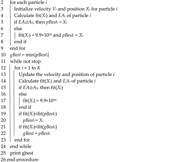
Function: PSO–BAS pseudo code in this example
Note: this example aims to solve the minimum value
Parameter: N is the population size
Processes 10 01479 i002
Table 4. The initial values of the algorithm parameters.
ParametersValue
SwarmSize30
Speed   weight   0.6
Inertia weight0.9
SelfAdjustmentWeight1.49
SocialAdjustmentWeight1.49
MaxIterations K175
Table 5. Algorithm comparison.
AlgorithmVariables, Results, or Evaluation Indicators
WeUeTECEAOperation Time
Grid search method8.56.50.11287080.8584266 s
PSO8.46.90.11278120.8601140 s
PSO–BAS8.47.20.31263050.87121 s
Table 6. The optimal 2D EW scheme (unit: years).
Ue/×104 KMWe/Years
2.54.56.58.510.5
2.50.73.12.53.13.7
4.50.10.10.10.10.1
6.50.10.10.10.10.1
8.50.10.10.10.10.1
10.50.70.70.70.70.7
Table 7. The EW cost (unit: 104 CNY/year).
Ue/×104 KMWe/Years
2.54.56.58.510.5
2.539.5739.1439.1139.1139.10
4.513.8313.1913.1413.1313.13
6.513.6212.9412.8912.8712.88
8.515.5514.9214.8814.8714.86
10.516.3616.2515.8716.6016.49
Table 8. The system availability.
Ue/×104 KMWe/Years
2.54.56.58.510.5
2.50.98960.99320.99150.99140.9917
4.50.95430.95020.94630.94450.9425
6.50.87620.87130.86780.86210.8584
8.50.76530.66100.66320.65870.7712
10.50.75380.73060.78510.73360.7413
Publisher’s Note: MDPI stays neutral with regard to jurisdictional claims in published maps and institutional affiliations.

