Abstract
Voltage sags are a serious problem within power supplies, which pose threats to both residential electricity and industrial manufacturing. Since any one sag may be recorded by multiple monitoring devices from different substations, the issue of redundant information in data arises. In this regard, a novel method for voltage sag events based on projection technology, shape dynamic time warping (shapeDTW), and spectral clustering is proposed. The main contributions of this paper may be summarized as follows: (1) We present a new method for extracting the voltage anomaly waveform, which is a fast projection segmentation algorithm (FPSA). The voltage sag waveform is only a part of the voltage anomaly waveform, so the voltage anomaly waveform contains more information. (2) ShapeDTW and spectral clustering are used to match and cluster voltage anomaly waveforms, so as to achieve the normalization of voltage sag events. (3) In practical engineering, the proposed method in the paper can be used to obtain the impact of voltage sags, reduce computational complexity, and ease the workload of the operation and maintenance engineers. Experiments were conducted using voltage sag data from voltage sag events recorded by the 10 kV monitoring points in Beijing, China. The results showed the effectiveness and reliability of our proposed methods.
1. Introduction
Currently, voltage sags have become an increasingly relevant issue for both utility companies and their consumers. In certain industries, a sag event only a few milliseconds in length can interrupt critical processes, which may then take several hours to be restarted. This results in large financial losses due to downtime [1]. Moreover, in industrial applications, voltage sags are the most frequently occurring disturbances among all the possible disturbances and account for 92% to 98% of interruptions. They may also be responsible for other disturbances in the power network [2]. Therefore, the treatment and research of voltage sags are important in improving the reliability of power systems and ensuring a safe power supply in industrial production and daily life [3]. The Institute of Electrical and Electronics Engineers’ (IEEE) definition for voltage sag is as follows: the root mean square (RMS) voltage drops to 10– of the rated value, and the duration is 10 ms–60 s [4]. At present, the data collection, detection, classification, and identification of voltage sags are the focus of research; see [5,6,7,8,9,10,11,12].
Many studies have been performed regarding the pattern recognition of voltage sags [3]. In general, there are three methods: data mining, signal processing, and physical modeling. Distinct methods for identifying the source of voltage sags were analyzed in [5], which are based on the disturbance energy, voltage current characteristic, or active current component. Reference [13] proposed a Kullback–Leibler divergence measure and standard deviation for voltage sag and harmonics identification. A support vector machine and support vector regression were used to identify fault types and estimate fault resistance. The Euclidean distance approach was used to identify the fault distance in [14]. K-means clustering was used to identify voltage sags in [15]. Reference [16] detected and classified different power quality disturbances using the half- and one-period windowing technique based on a continuous S-transform and neural networks. Several signal-processing techniques have been proposed for power quality (PQ) disturbance detection and segmentation. In [17], sags and interruptions were detected by the RMS value. Its main drawback is the poor results achieved with non-stationary signals due to the dependency of the RMS on both periodicity and wave shape. A sag/swell detection algorithm based on wavelet transform, operating even in the presence of flicker and harmonics in the voltage source, was presented in [18]. In [19], the Kalman filter and an expert system were used to segment and identify different types of voltage dips (fault-induced, transformer saturation, induction motor starting) and interruptions (non-fault and fault-induced). The main drawbacks of this method are related to either the failure in detecting very small changes in the voltage magnitude or the time resolution problems. In [20], a method for voltage sag source identification that combined wavelet analysis and modified dynamic time warping (DTW) distance was proposed. In [21], a statistical analysis of variance (MANOVA) was directly proposed to extract the attributes of voltage events from the voltage and current waveforms. In [22], Thevenin’s equivalent circuit was used to replace any power network. By determining the sign of the internal resistance in Thevenin’s equivalent circuit, the origin of a voltage sag disturbance could be easily identified. In [7], the authors proposed a method of detecting sags for applications in dynamic voltage restorers. The method is based on the fundamental amplitude calculation using the d-q components of each phase of the voltage signal in half-cycle windows. The method was efficient for different levels of sags, phase-jump, harmonics, and variation in fundamental frequency. In [23], the authors used the delayed Legendre wavelet, ant lion optimization algorithm, and a classifier ensemble to detect and classify eight types of sags.
The monitoring and analysis of voltage sag events can provide an effective scientific basis for power system operations management, accident investigation, fault location, and sag management [3]. With the advancement of science and technology, a large amount of original sampling data may be collected by monitoring systems. These data completely encapsulate the transient waveforms of each detected sag event. However, the data of the same voltage sag event would be recorded by multiple monitoring points. These data not only consume computer memory unnecessarily, but also leave higher workloads for engineers. The analysis of these data is then extremely inefficient due to a lack of effective data-processing procedures. Therefore, it is very important to identify whether the data recorded by different monitoring points are the voltage sag caused by the same event. As far as we know, there is no relevant literature on this aspect. In order to meet the needs of practical engineering applications, a novel clustering analysis method for voltage sag events is proposed in this paper. At present, all classification methods are mainly based on the characteristics of the voltage sag waveform. However, this waveform is only a part of the voltage anomaly waveform. The voltage anomaly waveform contains more information than the voltage sag waveform. Therefore, we propose a new method for extracting the voltage anomaly waveform instead of the voltage sag waveform, which is an FPSA. Then, we use shapeDTW and spectral clustering to match and cluster voltage anomaly waveforms, so as to achieve the normalization of voltage sag events.
The rest of this paper is organized as follows. In Section 2, our novel clustering analysis method for voltage sag events based on projection technology, shapeDTW, and spectral clustering is introduced. In Section 3, real data analyses are used to verify the effectiveness of the FPSA and clustering analysis method. The conclusions are summarized in Section 4.
2. Methodology
In this section, the PFSA is presented as an effective solution to correctly identify non-stationary and quasi-stationary states in the measured voltage waveforms. We further investigate the classification of voltage sag events by combining shapeDTW and spectral clustering. A total of twenty recording files of voltage sag events are available to this end, which are labeled as id 01, 02, ⋯, 20. These signals are events recorded by PQ instruments and contain both pre-trigger and post-trigger information. Figure 1 shows voltage data (id 01). Next, we mainly use id01 data to illustrate our proposed FPSA.
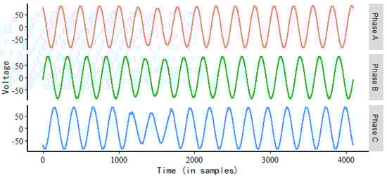
Figure 1.
Voltage data (id 01).
2.1. Fast Projection Segmentation Algorithm
The model used to detect a signal transition can be divided into three steps: signal modeling, acquisition of the detection parameter (DP), and extraction of the voltage anomaly segment. The basic principle of signal modeling is to generate residuals by comparing the actual responses with the expected responses of the system using mathematical models. These residuals are expected to be zero (or zero mean) under no-fault conditions. In practical situations, the residuals are corrupted by the presence of noise, unknown disturbances, and uncertainties in the system model. Hence, the aim of the method is to generate robust residuals that are insensitive to these noises and uncertainties, while remaining sensitive to faults. To this end, a simple and effective filtering method is proposed in this paper.
2.1.1. Signal Modeling Based on Filtering
Since the voltage data are usually periodic, it was assumed that the current voltage sag monitoring terminal records the data as K points/period ( in this paper). The voltage data of length N are expressed as , and then, the filtering method can be divided into the following three steps:
Given K, the original voltage data can be divided into L segments: , where , , , and denotes rounding down. Voltage data (id 01) segmentation results are shown in Figure 2, where the black dotted lines are the dividing lines.
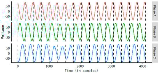
Figure 2.
Voltage data (id 01) are divided into L segments according to K.
According to IEEE Standard 1159–1995 [2], the RMS is used to initially determine whether has a sag. If is a sag, then is removed, where . The remaining data X after removal are obtained as follows.
Since the median can characterize the center position of the distribution and has the advantage of being robust and unaffected by outliers, we used the median of the data as the estimate of the lth column of the matrix X. Let = median , where . The process of Step 2 on the voltage sag data (id 01) is shown in Figure 3.
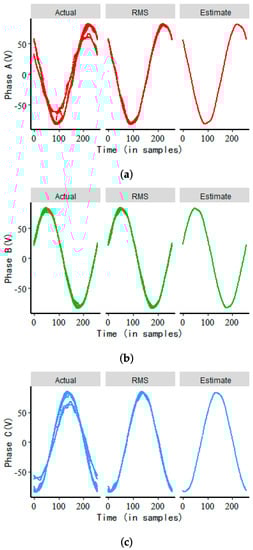
Figure 3.
The processing of Step 2 on voltage sag data (id 01), where “Actual” represents the actual response, “RMS” represents the real data after passing the RMS detection, “Estimate” represents , and the subfigures (a–c) represent the three-phase voltage sag data respectively.
Sequence 1 can be obtained by Step 2 as follows:
Repeat Sequence 1 on the length of the original data (N) to obtain Sequence 2:
Sequence 2 is our estimate of the original data. Then, we can obtain the filter sequence (residuals’ sequence) as follows:
The filtering process for voltage sag data (id 01) is shown in Figure 4.
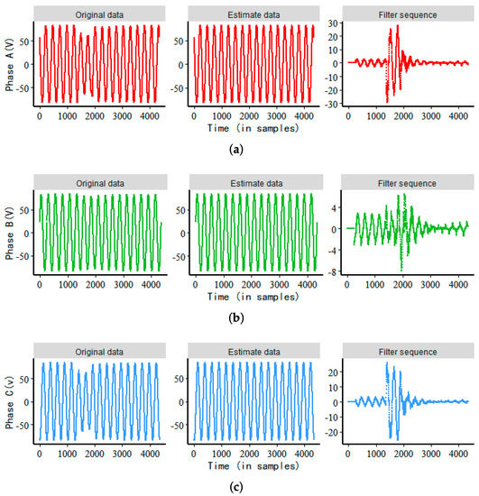
Figure 4.
The processing of Step 3 on voltage sag data (id 01), where subfigures (a–c) represent the three-phase voltage sag data respectively.
2.1.2. Detection Parameter Based on Sharp Drop Point
The voltage sag data are projected onto the vertical axis, and the frequency histogram can be obtained after projection (as shown in the red part of Figure 5b). The kernel density curve of the frequency histogram can be obtained by kernel density estimation (the red curve shown in Figure 5b). In the real data, the amount of voltage anomaly (voltage sag) data is always significantly smaller than the total amount of data. Based on this fact, we can clearly find that the anomaly data are mainly distributed in the tail region of the projection distribution, while the non-anomaly data are mainly concentrated in the central region of the projection distribution. The projected distribution of voltage sag data (id 01) is shown in Figure 5.
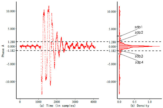
Figure 5.
Projection fast segmentation algorithm of A-phase voltage sag data (id 01), where (a) is the filter sequence of the A-phase (id 01) and (b) is the corresponding kernel density curve.
In this paper, we propose to use the local sudden-drop point (sdp) of the kernel density function as the basis for dividing the tail region and the central region of the kernel density curve, where the tail region of the kernel density curve is the anomaly data. In this way, the sdp is also called the DP. The local sudden-drop point of is defined as the location at which the density curve falls rapidly from high to low. A formal definition is given as follows.
Definition 1.
(Local sudden-drop point) For any point x, the interval is considered as the d-neighborhood of x. Then, is a local sudden-drop point if for all when ; see [24].
Remark 1.
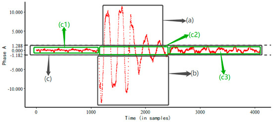
Through the definition of the sdp, we can conclude that if the voltage sags, the sdp of the kernel density function of the voltage data must exist, but there may be multiple sharp-drop points, such as sdp 1, sdp 2, sdp 3, and sdp 4 in Figure 6. In power data analysis, we can choose sdp 2 and sdp 3 as the division of the tail region and the central region of the kernel density function, where the region between sdp 2 and sdp 3 is the central region of the kernel density function.
Figure 6.
Region segmentation of the filter sequence (id 01).
2.1.3. Extracting Voltage Anomaly Segment
The region segmentation of the filtered sequence is shown in Figure 6. From Figure 6, we can see that the filtering sequence can be divided into three regions (a), (b), and (c) by sdp 2 and sdp 3. It is obvious that the voltage of the (a) and (b) regions has voltage anomalies. In fact, the voltage anomalies also occurred in the (c2) region of the (c) region. To this end, we propose a method for identifying the (c2) region in the (c) region as an anomaly region.
Through the above, a discontinuous voltage sequence can be obtained:
where the total number of sequences is n, . If the discontinuity distance between adjacent sequences is less than one period (K), we consider that the sequence point between the discontinuities has a sag, and based on the above method, the (c2) region in the (c) region can be identified as an anomaly.
Figure 7 shows the results of anomaly detection using the FPSA for voltage sag data (id 01), where the dashed lines indicate the respective start and end positions of the anomaly and the shaded portion is the anomaly segment. According to Figure 7, it can be concluded that the start and end positions of the A-phase are 1406 and 2694, respectively (those of the B-phase are 1405 and 2746 and the C-phase are 1404 and 2718).
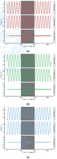
Figure 7.
FPSA for voltage sag data (id 01), where subfigures (a–c) represent the three-phase voltage sag data respectively.
2.2. Clustering Analysis of Voltage Sag Events
In this section, shapeDTW and spectral clustering are used to match and cluster voltage anomaly waveforms, so as to achieve the normalization of voltage sag events. The clustering analysis method is mainly divided into two steps. The first step uses shapeDTW to calculate the shape similarity between the anomaly curves extracted by the FPSA. The second step uses the obtained similarity values from the first step to construct the similarity matrix of spectral clustering, and then, the voltage anomaly curve is classified by spectral clustering.
2.2.1. Waveform Matching Based on Shapedtw
The DTW was first introduced in the 1970’s for audio analysis by [25,26] before being used for general time series analysis. By minimizing the cumulative distance between the signals and (time series), DTW provides a non-linear alignment optimal path between these two time series. It is a relatively straightforward process that first estimates the distance map between the signals with elements given by:
A cumulative distance map with elements is then computed from the distance map . represents the minimal accumulated distance to reach the point starting from the origin . It is given by:
where we have the following initial conditions:
This cumulative distance is used to define a warping path between signals and , denoted
verifies several constraints:
- The monotonicity constraint guarantees the time ordering.
- The boundary constraints: and .
- The step size conditions: and ; see Equation (3).
This path minimizes the final cumulative distance. Its length S depends on the signals to be aligned and is determined during the DTW process.
Figure 8 presents two examples of DTW alignments between two time series, with Figure 8a,b showing the alignments between series and Figure 8c,d showing the cumulative distance maps D and the warping paths in green for these two examples.
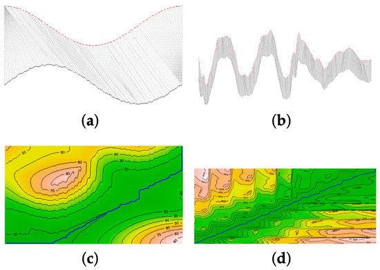
Figure 8.
Illustration of a DTW process for aligning two pairs of signals (one per column). The first row: the matching between points of two pairs of signals (in red and black) is symbolized by grey lines. The second row: superimposition of the warping path on the cumulative distance matrix D. Yellow areas of D correspond to larger cumulative distances, whereas green ones correspond to smaller ones. The first case of alignment (a,c) is an example of speech data. The second case of alignment (b,d) is an example of voltage sag data. The two pairs of signals are the phase A of voltage sag data id 01 and 02, respectively.
Although DTW obtains a global optimal solution, it does not necessarily achieve locally sensible matchings. Concretely, two temporal points with entirely dissimilar local structures may be matched by DTW. To address this problem, [27] proposed an improved alignment algorithm, named shape dynamic time warping (shapeDTW), which enhances DTW by taking pointwise local structural information into consideration.
ShapeDTW is a temporal alignment algorithm, which consists of two sequential steps: Firstly, represent each temporal point by some shape descriptor, which encodes structural information of local subsequences around that point; in this way, the original time series is converted into a sequence of descriptors. Secondly, use DTW to align two sequences of descriptors. The shapeDTW time series alignment procedure is shown in Figure 9 [27]. This section mainly uses the shapeDTW algorithm to calculate the shape similarity between voltage sag sequences extracted by the FPSA.
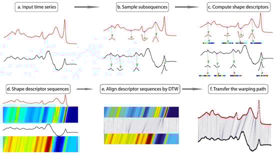
Figure 9.
Pipeline of shapeDTW. shapeDTW consists of two major steps: encode local structures by shape descriptors, and align descriptor sequences by DTW. Concretely, we sample a subsequence from each temporal point and further encode it by some shape descriptor. As a result, the original time series is converted into a descriptor sequence of the same length. Then, we align two descriptor sequences by DTW and transfer the found warping path to the original time series.
Remark 2.
Reference [27] gave fourshape descriptors: piecewise aggregate approximation (PAA), discrete wavelet transform (DWT), slope, and derivative. Derivative is used in this paper.
2.2.2. Spectral Clustering Based on shapeDTW
The spectral clustering algorithm is based on the spectral theory of graph theory and is widely used in image segmentation, computer vision, and pattern recognition. Spectral clustering is a class of methods based on eigen-decompositions of graph affinity matrices. Given a set of data points , a weighted graph is first constructed for which every vertex corresponds to a point in S and each edge is weighted by the similarity between the connected points. The Laplacian graph [28] is then derived from the adjacent matrix of G, and the eigenvectors of are computed. Finally, the traditional K- method is applied to the low-dimensional representations of the original data. There are many spectral clustering algorithms that are based on the above procedures [29,30,31].
In this paper, our proposed shapeDTW spectral clustering algorithm is developed in the Jordan–Weiss (NJW) framework [31]. Therefore, the NJW algorithm is briefly reviewed as Algorithm 1, for the sake of completeness. Algorithm 1 mainly involves the determination of the number of clusters k, the calculation of affinity matrix W, and the calculation of Laplacian matrix L.
| Algorithm 1: NJW spectral clustering algorithm. |
Input: Dataset in and the number of clusters k Output:k-way partition of the input data Construct the affinity matrix :
|
(1) There are mainly three methods for determining the number of clusters k: elbow method, average silhouette method, and gap statistic method. In this paper, we adopted the average silhouette method for determining the number of clusters k.
(2) The methods for calculating the affinity matrix are mainly the -neighborhood graph, k-nearest neighbor graph, and fully connected graph. In this paper, the fully connected graph is used to calculate .
where represents the Euclidean distance between and . In this paper, and represent the voltage filtering sequence. Since the lengths of and are different, the Euclidean distance between and cannot be calculated. For this, we used the shapeDTW similarity between and instead of the Euclidean distance between and . Then,
where shapeDTW represents the shapeDTW similarity between and . We aimed to improve spectral clustering by shapeDTW, so that it can cluster datasets of voltage filtering sequences.
(3) There are mainly three methods for the calculation of Laplacian matrices : unnormalized Laplacian matrices, random walk Laplacian matrices, and symmetric Laplacian matrices [29]. In this paper, we adopted symmetric Laplacian matrices, so:
2.3. Procedure Flow Chart of the Methodology
A procedure flow chart of the proposed methodology is presented in Figure 10.
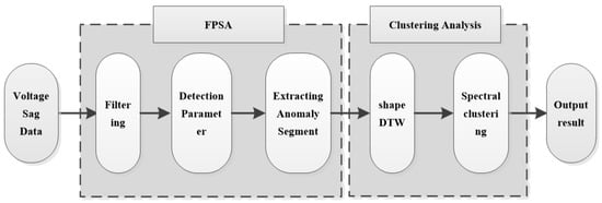
Figure 10.
Procedure flow chart of the methodology.
3. Empirical Analysis
3.1. Data
To verify the effectiveness of the method proposed in this paper, real data samples from a voltage sag monitoring system were selected. These data recorded the voltage sag events that occurred in Beijing in May 2018. In total, twenty valid samples were retained after excluding invalid samples. These samples belonged to three types of sag events. The sag types and number of data samples are shown in Table 1. According to the process in Figure 10, firstly, the start position and end position of the anomaly of the voltage sag data are detected. Secondly, the anomaly waveform is extracted. Thirdly, the anomaly waveform is classified to achieve the classification purpose of the voltage sag events.

Table 1.
The sag types and number of data samples.
3.2. Empirical Results
To illustrate the accuracy of the FPSA detection results, we compared the FPSA with the RMS method [16]. The results are shown in Table 2, where “RMS” represents the root mean square of the half-period refresh voltage detection method and “FPAS” represents the FPSA. The formula for calculating the RMS is as follows:
where N is the number of sampling points per period (), is the instantaneous value of the voltage waveform acquired for the time, and k is the calculated window (). The threshold of the detection voltage was set to 0.9 pu according to the definition of a voltage sag.
Table 2.
Detection results of voltage ( [start position, stop position]).
From Table 2, we can conclude that the sag segments detected by the RMS are all inside the abnormal segment detected by the FPSA, so the abnormal segment contains more information than the sag segment. Therefore, it is reasonable to use the abnormal segment for clustering analysis of the voltage sag events.
We used the method proposed in this paper to cluster the voltage sag events for A-phase voltage data, B-phase voltage data, and C-phase voltage data in the voltage sag data, respectively. The results of the clustering analysis of A-phase voltage data, B-phase voltage data, and C-phase voltage data are shown in Table 3, Table 4 and Table 5 and Figure 11, Figure 12 and Figure 13, respectively. Table 3, Table 4 and Table 5 is an affinity matrix (, ) calculated using the abnormal waveform segment of the A-phase (B-phase, C-phase) voltage data. The area of the same color (gray, green, and yellow) in (, ) represents the voltage sag caused by the same event. The calculation method of (, ) is in Equation (7). Figure 11, Figure 12 and Figure 13 show the clustering results of the abnormal voltage segments in the A-phase (B-phase, C-phase) voltage data.
Table 3.
The affinity matrix .
Table 4.
The affinity matrix of B-phase voltage sag data.
Table 5.
The affinity matrix of C-phase voltage sag data.
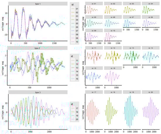
Figure 11.
Clustering result based on A-phase voltage sag data.
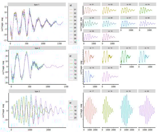
Figure 12.
Clustering result based on B-phase voltage sag data.
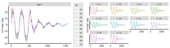
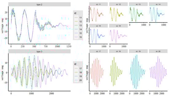
Figure 13.
Clustering result based on C-phase voltage sag data.
From Table 3, Table 4 and Table 5, we can see that the value of the same color area is obviously larger than the value of the blank area, indicating that the abnormal waveform segment of the voltage sag caused by the same event is more similar. It can be obtained from Figure 11, Figure 12 and Figure 13 that the clustering accuracy of the clustering analysis method proposed in this paper is 100% for the voltage sag data (id 01–20).
Table 6 shows the clustering results of the affinity matrix of different abnormal voltage segments using the average of the affinity matrix of the voltage data of phase A, phase B, and phase C, where . has the same clustering results as , , and .
Table 6.
The affinity matrix of voltage sag data.
The results of the above empirical analysis show that the proposed method can effectively achieve the clustering of voltage sag events.
4. Concluding Remarks
With the development of electrical power technology and expansions of the monitoring scope, the amount of voltage sag data has also dramatically increased over time. The increase in the amount of voltage sag data generates a huge amount of work for power engineers due to the need for the analysis of the data. In addition, accurate clock synchronization between voltage sag events is difficult to achieve due to the costs of monitoring such power systems. Therefore, it is impossible to know whether the voltage sag events detected by different monitoring stations correspond to the same event. Therefore, valid information cannot be processed in time, and valuable information is discarded. The clustering analysis method proposed in this paper is effective in solving this problem, and the test results obtained based on real data reflect the accuracy of the approach. The voltage anomaly waveform of voltage sags caused by the same event has a high degree of similarity, and the voltage anomaly waveform of the voltage sags caused by different events is significantly different. Our method can effectively judge whether voltage sags detected by different monitoring points were caused by the same event. The range of influence of the voltage sag event can be obtained simultaneously.
Author Contributions
Conceptualization, J.J. and C.H.; methodology, C.H.;. software, J.J.; writing—original draft preparation, J.J. writing—review and editing, C.H. All authors have read and agreed to the published version of the manuscript.
Funding
This research received no external funding.
Institutional Review Board Statement
Not applicable.
Informed Consent Statement
Not applicable.
Data Availability Statement
Not applicable.
Acknowledgments
The authors would like to thank Nanjing Shining Electric Automation Co., Ltd. for providing the field measurement waveforms. Nanjing Shining Electric Automation supported the development of the proposed method for power quality monitoring systems.
Conflicts of Interest
The authors declare no conflict of interest.
References
- Vegunta, S.C.; Milanovic, J.V. Estimation of cost of downtime of industrial processdue to voltage sags. IEEE Trans. Power Deliv. 2011, 26, 576–587. [Google Scholar] [CrossRef]
- Arias-Guzman, S. Analysis of voltage sag severity case study in an industrial circuit. IEEE Trans. Ind. Appl. 2017, 53, 15–21. [Google Scholar] [CrossRef]
- Mei, F.; Ren, Y.; Wu, Q.; Zhang, C.; Pan, Y.; Sha, H.; Zheng, J. Online recognition method for voltage sags based on a deep belief network. Energies 2018, 12, 43. [Google Scholar] [CrossRef] [Green Version]
- Xiao, X.Y.; Chen, Y.Z.; Wang, Y.; Ma, Y.Q. Multi-attribute analysis on voltage sag insurance mechanisms and their feasibility for sensitive customers. Iet. Gener. Transm. Dis. 2018, 12, 3892–3899. [Google Scholar] [CrossRef]
- Polajzer, B.; Tumberger, G.S.; Seme, S.; Dolinar, D. Detection of voltage sag sources based on instantaneous voltage and current vectors and orthogonal Clarke’s transformation. IET Gener. Transm. Distrib. 2008, 2, 219–226. [Google Scholar] [CrossRef]
- Kezunovic, M.; Liao, Y. A new method for classification and characterization of voltage sags. Electr. Pow. Syst. Res. 2001, 58, 27–35. [Google Scholar] [CrossRef]
- Sadigh, A.K.; Smedley, K.M. Fast and precise voltage sag detection method for dynamic voltage restorer (DVR) application. Electr. Pow. Syst. Res. 2016, 130, 192–207. [Google Scholar] [CrossRef]
- Xi, Y.; Li, Z.; Zeng, X.; Tang, X.; Liu, Q.; Xiao, H. Detection of power quality disturbances using an adaptive process noise covariance Kalman filter. Digit. Signal. Process. 2018, 76, 34–49. [Google Scholar] [CrossRef]
- Saini, M.K.; Beniwal, R.K. Detection and classification of power quality disturbances in wind-grid integrated system using fast time-time transform and small residual-extreme learning machine. Int. Trans. Electr. Energy Syst. 2018, 28, e2519. [Google Scholar] [CrossRef]
- Jeevitha, S.R.S.; Mabel, M.C. Novel optimization parameters of power quality disturbances using novel bio-inspired algorithms: A comparative approach. Biomed. Signal Process. Control. 2018, 42, 253–266. [Google Scholar] [CrossRef]
- Branco, H.M.; Oleskovicz, M.; Coury, D.V.; Delbem, A.C. Multiobjective optimization for power quality monitoring allocation considering voltage sags in distribution systems. Int. J. Electr. Power Energy Syst. 2018, 97, 1–10. [Google Scholar] [CrossRef]
- Bagheri, A.; Gu, I.; Bollen, M.; Balouji, E. A Robust Transform-Domain Deep Convolutional Network for Voltage Dip Classification. IEEE Trans. Power Deliv. 2018, 33, 2794–2802. [Google Scholar] [CrossRef] [Green Version]
- Kapoor, R.; Gupta, R.; Jha, S.; Kumar, R. Boosting performance of power quality event identification with KL Divergence measure and standard deviation. Measurement 2018, 126, 134–142. [Google Scholar] [CrossRef]
- Gururajapathy, S.S.; Mokhlis, H.; Illias, H.A.; Awalin, L.J. Support vector classification and regression for fault location in distribution system using voltage sag profile. IEEE J. Trans. Electr. Electron. Eng. 2017, 12, 519–526. [Google Scholar] [CrossRef]
- Garcia-Sánchez, T.; Gómez-Lázaro, E.; Muljadi, E.; Kessler, M.; Muñoz-Benavente, I.; Molina-Garcia, A. Identification of linearised RMS-voltage dip patterns based on clustering in renewable plants. IET Gener. Transm. Distrib. 2018, 12, 1256–1262. [Google Scholar]
- Daud, K.; Abidin, A.F.; Ismail, A.P. Voltage Sags and Transient Detection and Classification Using Half/One-Cycle Windowing Techniques Based on Continuous S-Transform with Neural Network. In Proceedings of the 2nd International Conference on Applied Physics and Engineering (ICAPE), Penang, Malaysia, 2–3 November 2016. [Google Scholar]
- Meena, P.; Rao, K.U.; Ravishankar, D. A modified simple algorithm for detection of voltage sags and swells in practical loads. IEEE Int. Conf. Power Syst. 2009, 12, 1–6. [Google Scholar]
- Latran, M.B.; Teke, A. A novel wavelet transform based voltage sag/swell detection algorithm. Int. J. Electr. Power Energy Syst. 2015, 71, 131–139. [Google Scholar] [CrossRef]
- Styvaktakis, E.; Bollen, M.H.; Gu, I.Y. Expert system for classification and analysis of power system events. IEEE Trans. Power Deliv. 2002, 17, 423–428. [Google Scholar] [CrossRef]
- Chu, J.W.; Yuan, X.D.; Chen, B.; Wang, X.C.; Qiu, H.F.; Gu, W. A Method for Distribution Network Voltage Sag Source Identification Combining Wavelet Analysis and Modified DTW Distance. Power Syst. Technol. 2018, 42, 637–643. [Google Scholar]
- Nunez, V.B.; Velandia, R.; Hernandez, F.; Melendez, J.; Vargas, H. Relevant Attributes for Voltage Event Diagnosis in Power Distribution Networks. Rev. Iberoam. Autom. Inform. Ind. 2013, 10, 73–84. [Google Scholar]
- Tang, Y.; Wei, R.; Chen, K.; Fang, Y. Voltage sag source identification based on the sign of internal resistance in a “Thevenin’s equivalent circuit”. Int. Trans. Electr. Energy Syst. 2017, 27, e2461. [Google Scholar] [CrossRef]
- Saini, M.K.; Aggarwal, A. Fractionally delayed Legendre wavelet transform based detection and optimal features based classification of voltage sag causes. J. Renew. Sustain. Energy 2019, 11, 25–36. [Google Scholar] [CrossRef]
- Zhuang, D.; Liu, Y.; Liu, S.; Ma, T.; Ong, S.H. A shape-based cutting and clustering algorithm for multiple change-point detection. J. Comput. Appl. Math. 2020, 6, 112623. [Google Scholar] [CrossRef]
- Rabiner, L.R. Considerations in dynamic time warping algorithms for discrete word recognition. J. Acoust. Soc. Am. 1978, 63, 575–582. [Google Scholar] [CrossRef]
- Sakoe, H.; Chiba, S. Dynamic programming algorithm optimization for spoken word recognition. IEEE Trans. Acoust. 1978, 26, 43–49. [Google Scholar] [CrossRef] [Green Version]
- Zhao, J.P.; Laurent, I. Shapedtw: Shape dynamic time warping. Pattern Recogn. 2018, 74, 171–184. [Google Scholar] [CrossRef] [Green Version]
- Chung, F.R.K. Spectral Graph Theory, Regional Conference Series in Mathematics. AMS 1997, 92, 142–162. [Google Scholar]
- Luxburg, U. A tutorial on spectral clustering. Stat Comput. 2007, 17, 395–416. [Google Scholar] [CrossRef]
- Shi, J.; Malik, J. Normalized cuts and image segmentation. IEEE Trans. Pattern Anal. Mach. Intell. 2000, 22, 888–905. [Google Scholar]
- Ng, A.; Jordan, M.; Weiss, Y. On spectral clustering: Analysis and an algorithm. In Advances in Neural Information Processing Systems (NIPS); MIT Press: Cambridge, MA, USA, 2002; Volume 17. [Google Scholar]
Publisher’s Note: MDPI stays neutral with regard to jurisdictional claims in published maps and institutional affiliations. |
© 2022 by the authors. Licensee MDPI, Basel, Switzerland. This article is an open access article distributed under the terms and conditions of the Creative Commons Attribution (CC BY) license (https://creativecommons.org/licenses/by/4.0/).