Strengthening Criteria Independence through Optimization of Alternative Value Ratio Comparisons

Abstract

Every decision maker’s internal scale is different based on a myriad of possible factors unique to that decision maker. Conflicting criteria within and between alternatives in multicriteria decision making can create negative effects within the weighting schemes and amplify preference biases and scale disparities between decision makers in a group decision context. Additionally, the weighting of group decision-making frameworks can intensify the already skewed criteria values. When making judgments against requirements, it may be preferable to reduce scale trend distortions between decision makers as much as possible. Previous research supports that certain information presentation modes can significantly reduce preference bias and strengthen criteria independence against requirements through cross alternative anchoring. This paper expands that research and proposes a new optimization model for strengthening criteria independence and consensus in group decision making. Initial results indicate the proposed optimization model can significantly reduce scale distortions and smooth comparative alternative value trends between decision makers toward strengthened group consensus. Furthermore, results support the potential and opportunity for semiautonomous group consensus processes.

1. Introduction

Group decision making (GDM) in a multicriteria scenario is extremely sensitive to internal and external influences. Many factors affect how each individual assigns criteria scores, including personal experience with and preference for alternatives, varying expertise in criteria, baseline requirements, and as demonstrated in previous experiments, information presentation modes. Mode or judgement format is also considered to be one of the four essential issues in GDM [1]. These factors, if not carefully considered, can have significant effects on judgement and result in biased responses and violations of a critical assumption of multicriteria decision making (MCDM): criteria independence. Mode affects the dimensions in which decision makers anchor and adjust judgement in pairwise comparisons. It also affects the type and amount of response bias. Furthermore, mode has been shown to influence the response scale and the decision process in comparing alternatives. Frederick and Mochon [2] refer to this personal change in response scale as scale distortion.

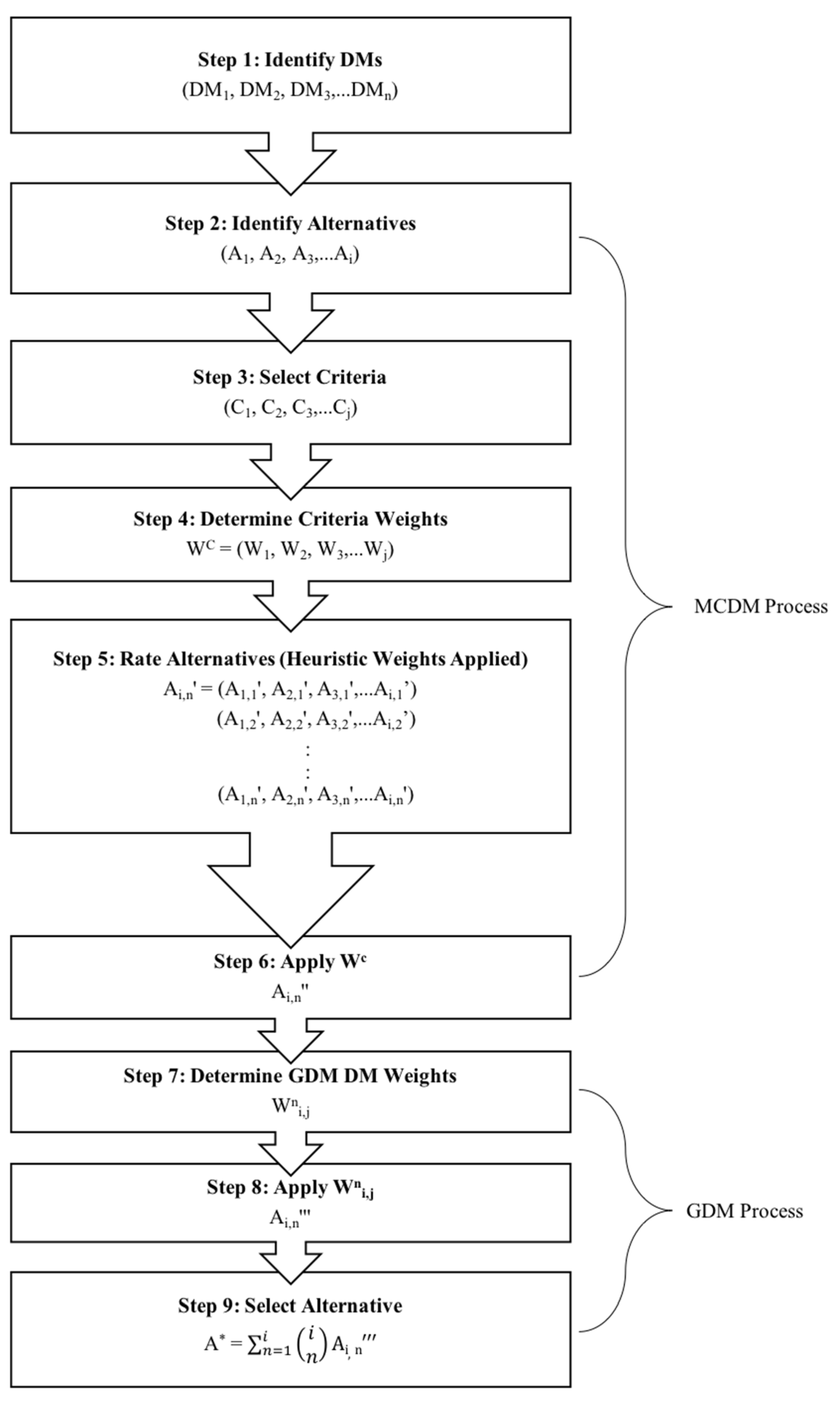
Another essential component of GDM is weighting. There are many proposed decision flow charts for MCDM considering GDM. We propose the flow chart shown in Figure 1 as a general process that includes multiple layers of criteria and DM weighting. During the decision process, multiple different phases of weighting occur. However, a key phase not generally accounted for in the formal process is internal to the decision maker and occurs during the rating of alternatives in step 5. We refer to this account of weighting as heuristic weighting.

Figure 1. Multicriteria GDM process.

Any resulting bias from step 5 can create an inappropriate imbalance in criteria scores within alternatives and/or across alternatives. It is these types of functional dependencies [3] that are difficult to characterize. Dependence between alternatives and within criteria and corresponding requirements is natural. Independence across criteria and corresponding requirements is ideal. Methods to identify and correct for dependencies in decision contexts are generally unaccounted for in traditional MCDM. 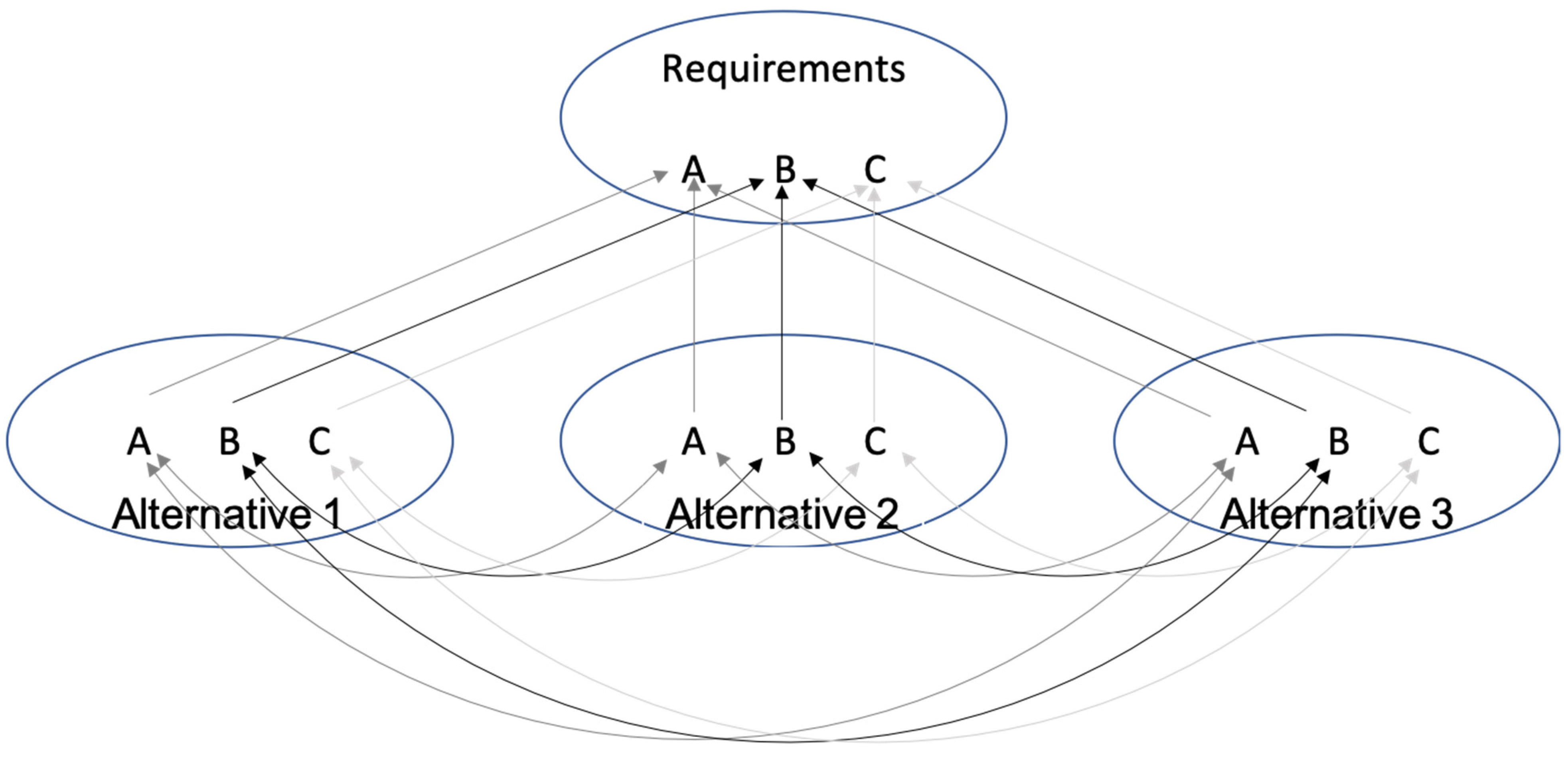Figure 2 depicts this type of scenario. As shown, there are three alternatives judged against requirements for each criterion A, B, and C. Alternatives 1, 2, and 3 are interdependent within criteria and within criteria requirements. Criteria A, B, and C are independent of each other.

Figure 2. Ideal decision context against requirements.

If dependencies cross criteria boundaries and criteria are weighted through steps 6 and 8, bias effects are compounded and cascaded through the process. It is difficult to trust judgement and weighted scores if criteria are not judged independently of each other. Requirements, whether informal or formal, biased or unbiased, are often used as supporting benchmarks to guide the decision maker in the direction of stronger criteria independence. However, it is a misconception that detailed decision, alternative, and criteria requirements alone are a sufficient mechanism to reduce bias and strengthen criteria independence. This research supports the idea that strategic facilitation through mode affects not only heuristics but also method of alternative comparison. Results support that when using a mixed mode of information presentation and evaluation, as described in Table 1, subjects not only make alternative comparisons using ratio scaling, but compatible decision makers (having identical hierarchies of alternatives) use significantly similar ratios regardless of scale range.

Table 1. Mode descriptions.

Mode	Description
Joint	Alternatives and criteria are presented and judged side by side
Separate	Alternatives and criteria are presented and judged separately (sequentially)
Mixed	Alternatives presented and judged side by side within criterion. Different criteria presented and judged separately (sequentially)

If mode is to complement the criteria weighting method, the facilitation and formulations established in Step 5 of the process is critical. DMs can be influenced by a multitude of factors when determining criteria values. When comparing criteria against specific requirements, it is ideal that criteria considerations are independent of each other and match requirement criteria. For example, the value of the price of an alternative should be determined only by the limitations established by the price requirements, and not how other criteria such as performance do or do not justify the price. If the latter occurs, it is extremely difficult to determine weight accuracy of criteria as they satisfy requirements within decision makers. Certainly, a lack of criteria independence will cloud and skew the weighting of individual criteria and cascade effects through the GDM weighting. This makes the marrying of strategic decision facilitation and weighting methods imperative to reduce the negative effects of conflicting criteria.

2. Scale Distortion

Anchoring is a scaling effect in that the anchor changes how the response scale is used [2]. These experiments provided evidence that anchoring effects are significant when making sequential judgements comparing different items, especially amongst those with high conceptual similarity, on the same scale. In contrast, there is also evidence that anchoring effects are minimized when making sequential judgments about different items using different scales [2].

In most situations, use of the same scale is unavoidable. When a decision maker has to compare alternatives with high conceptual similarity side by side, such as choosing the better consumer product in a single-objective or multiobjective scenario, identical scales are natural between alternatives and corresponding criteria. Additionally, in most circumstances, and in the case of the research presented in this article, alternatives are competing and so are considered to have high conceptual similarity. Regardless of a predefined scale, every decision maker defines the range within that scale differently. A 7 out of 10 to one decision maker may be a 5 out of 10 to another based on personal values and experiences. Furthermore, how a decision maker assigns value in pairwise comparisons determines the range utilized within the full range of the scale. Therefore, value cannot be determined in relation to the full scale. Value should be determined by the comparison ratios of alternative scores regardless of the potential value set in the range. This is especially true when aggregating and weighting scores from multiple decision makers in a GDM context. It has been shown that a DM calculates a ratio when making pairwise comparisons of alternatives [4,5]. Furthermore, current MCDM methods such as the analytic hierarchy process (AHP) make relative comparisons of alternatives based on ratio scaling [6].

Results from previous sections support that when presented alternatives in mixed mode, compatible subjects assigned value using significantly similar ratio comparisons regardless of scale range. Additionally, there was a disproportionate difference in the numbers of subjects in the subgroup that rated alternatives in the ideal rank order as they compared to requirements to subgroups that were deemed to have extreme amount of bias (i.e., last alternative was ranked first and/or first alternative was ranked last). That is, subjects with lower amounts of bias in their responses far outnumbered subjects with extreme bias in mixed mode. Therefore, there is evidence that scales are distorted from judgement of the first alternative and adjusted using similar ratios amongst compatible decision makers in mixed mode. In addition, evidence of extreme bias is significantly less prevalent in mixed mode.

Even in situations when mode reduces preference bias and consensus is reached in hierarchy of alternatives, unbalanced scale distortions between decision makers can remain. This is due to both criteria dependence and limitations of the scoring scales. This in turn causes misrepresentation of true criteria values as they satisfy criteria requirements. This is not to say that scores among decision makers should be as close as possible; however, it can be argued that the differences between alternative scores within decision makers should reflect similar ratios to other decision makers.

Consider a group decision scenario with a set $N\left(A\right)$ of alternatives, a set $N\left(DM\right)$ of decision makers (DMs), and a set N($C)$ of criteria. Now consider the following case: $N\left(A\right)=3$ alternatives (i = 1, …, 3), $N\left(DM\right)$ decision makers (m = 1, …, $N\left(DM\right)$), and $N\left(C\right)$ criteria (j = 1, …, $N\left(C\right)$). Since ratios are being considered, define ${\rho }_x^m$ ($x=1, 2$) as the ratio of scores $a_i^m$/$a_1^m$(i = 2, …, $N\left(A\right)$; m = 1, …, $N\left(DM\right)$) between alternatives $A_i^m$ and $A_1^m$ for i = 2, …, $N\left(A\right)$. Ratios are always baselined from the score of the same alternative, in this case the score $a_1^m$ of $A_1^m$. For three alternatives, there are x = 2 ratios for each criterion and decision maker. Thus, there are $N\left(A\right)-1$ unique ratios. 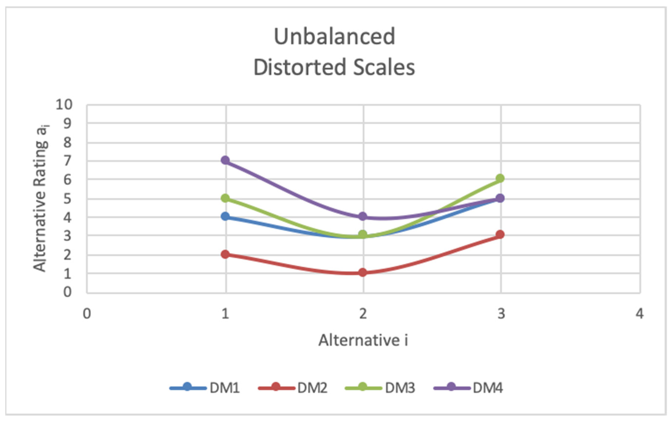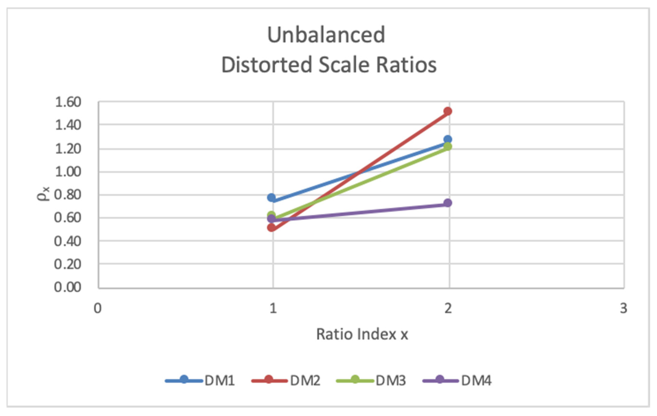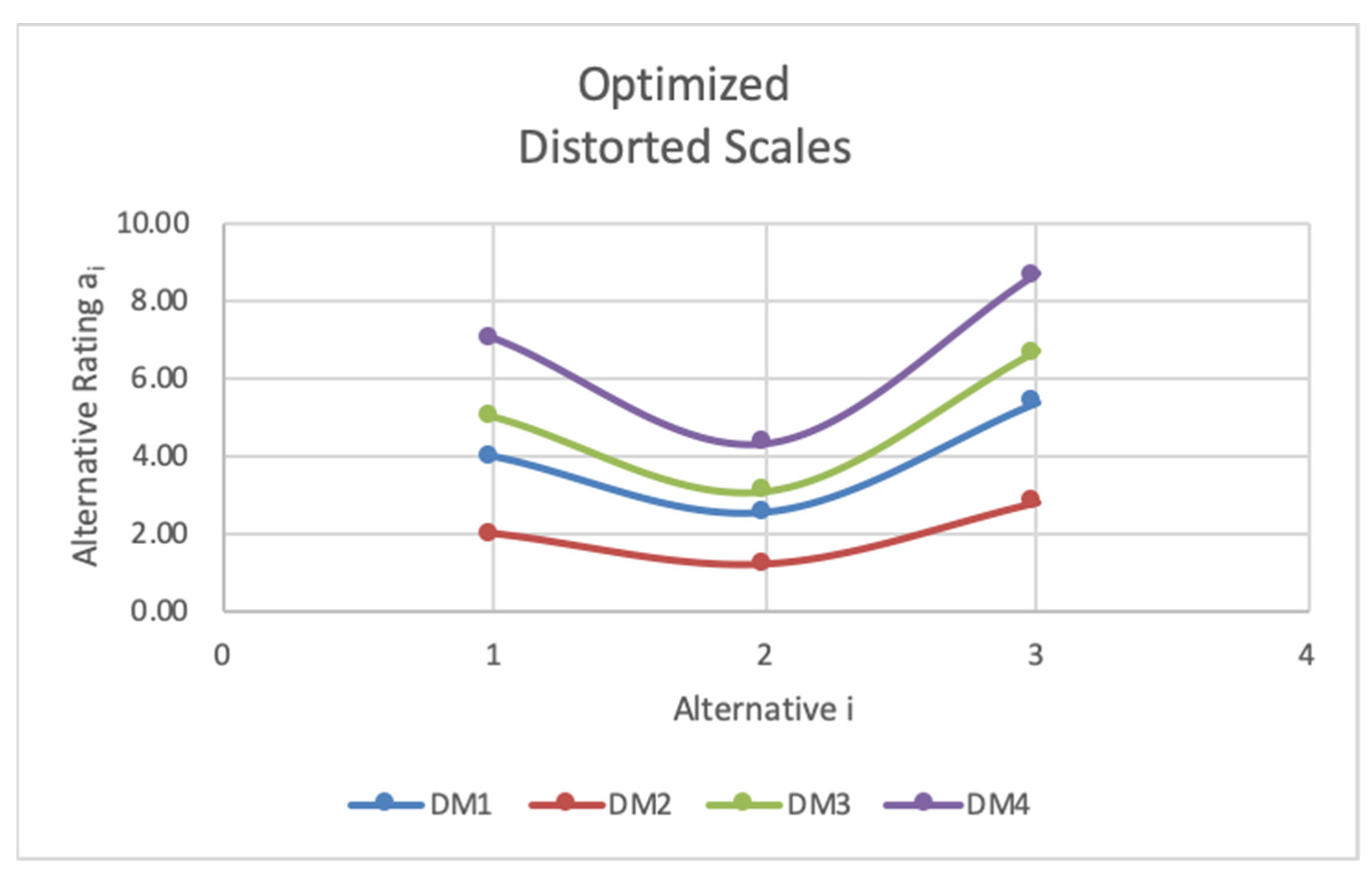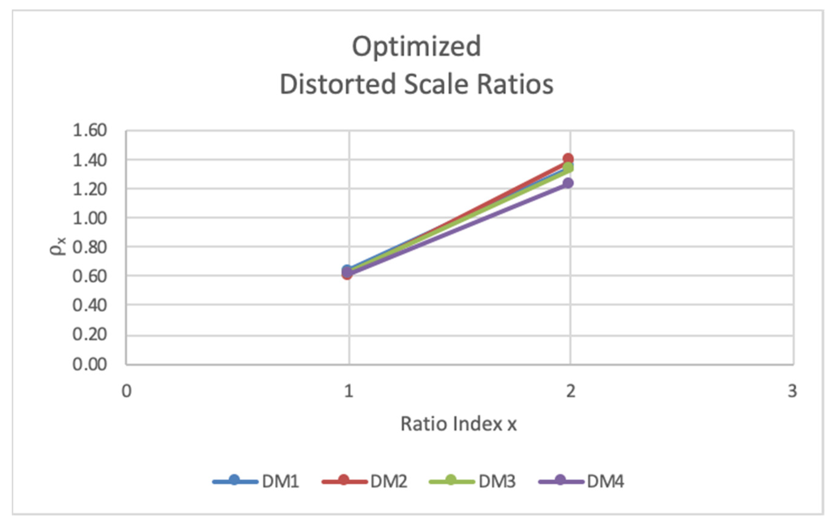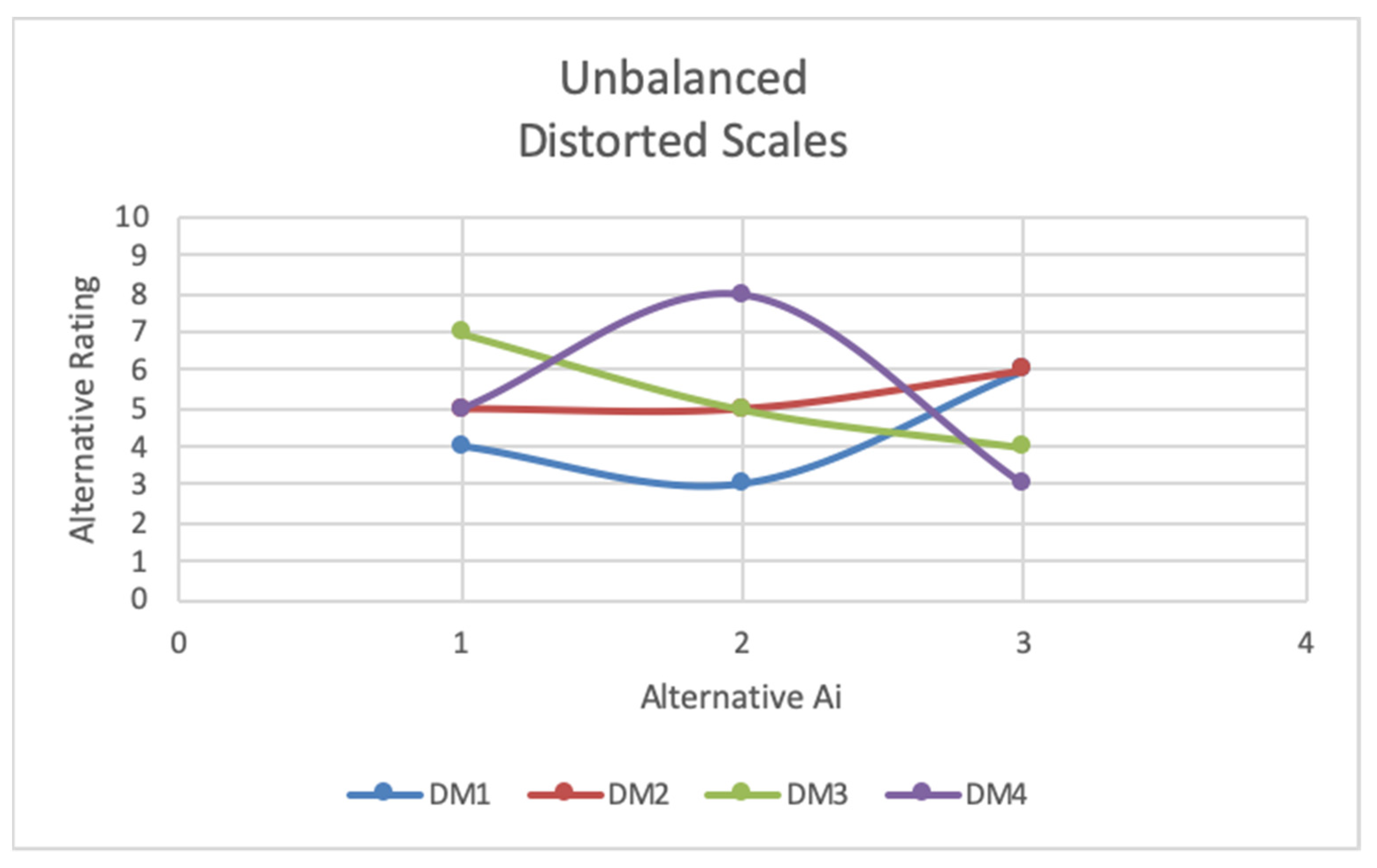Figure 3 and Figure 4 depict scale trend distortions between four ($N\left(DM\right)=4$) DMs across hypothetical judgements of three ($N\left(A\right)=3$) alternatives for a single criterion.

Figure 3. Unbalanced distorted scale scores between decision makers for a criterion.

Figure 4. Unbalanced distorted scale ratios between decision makers.

Although the trends in the alternative $A_i$ scores seem relatively similar in Figure 3, closer inspection of the ratios ${\rho }_x^m$ for DM_m in Figure 4 reveal there is an imbalance between DMs. Ratios ${\rho }_1^m$ (A₂/A₁) are relatively close between DMs; however, ratios ${\rho }_2^m$ (A₃/A₁) are much further apart, and ${\rho }_2^4<1.0$, which indicates a disagreement in hierarchy and a potential issue with criteria independence. 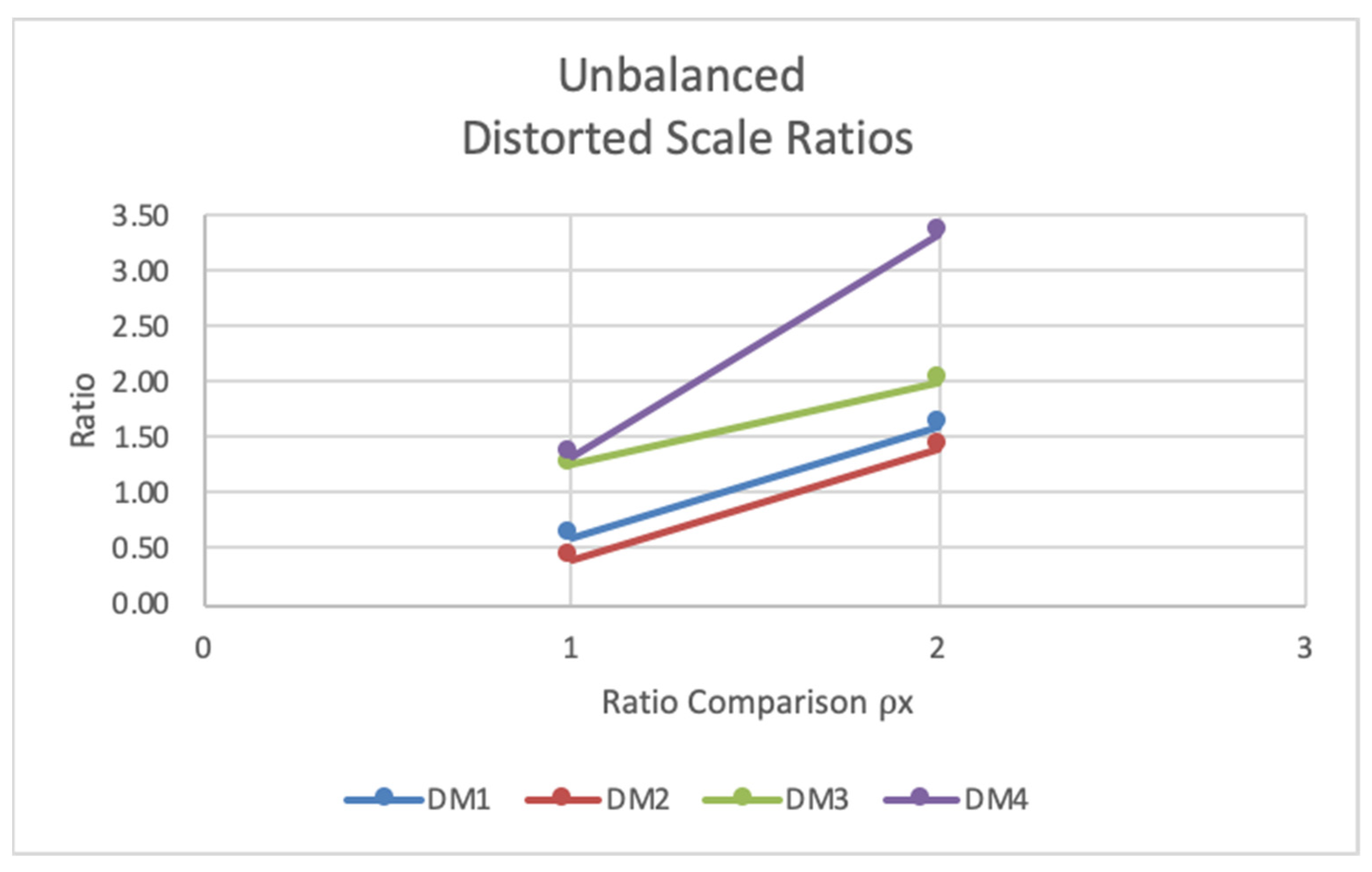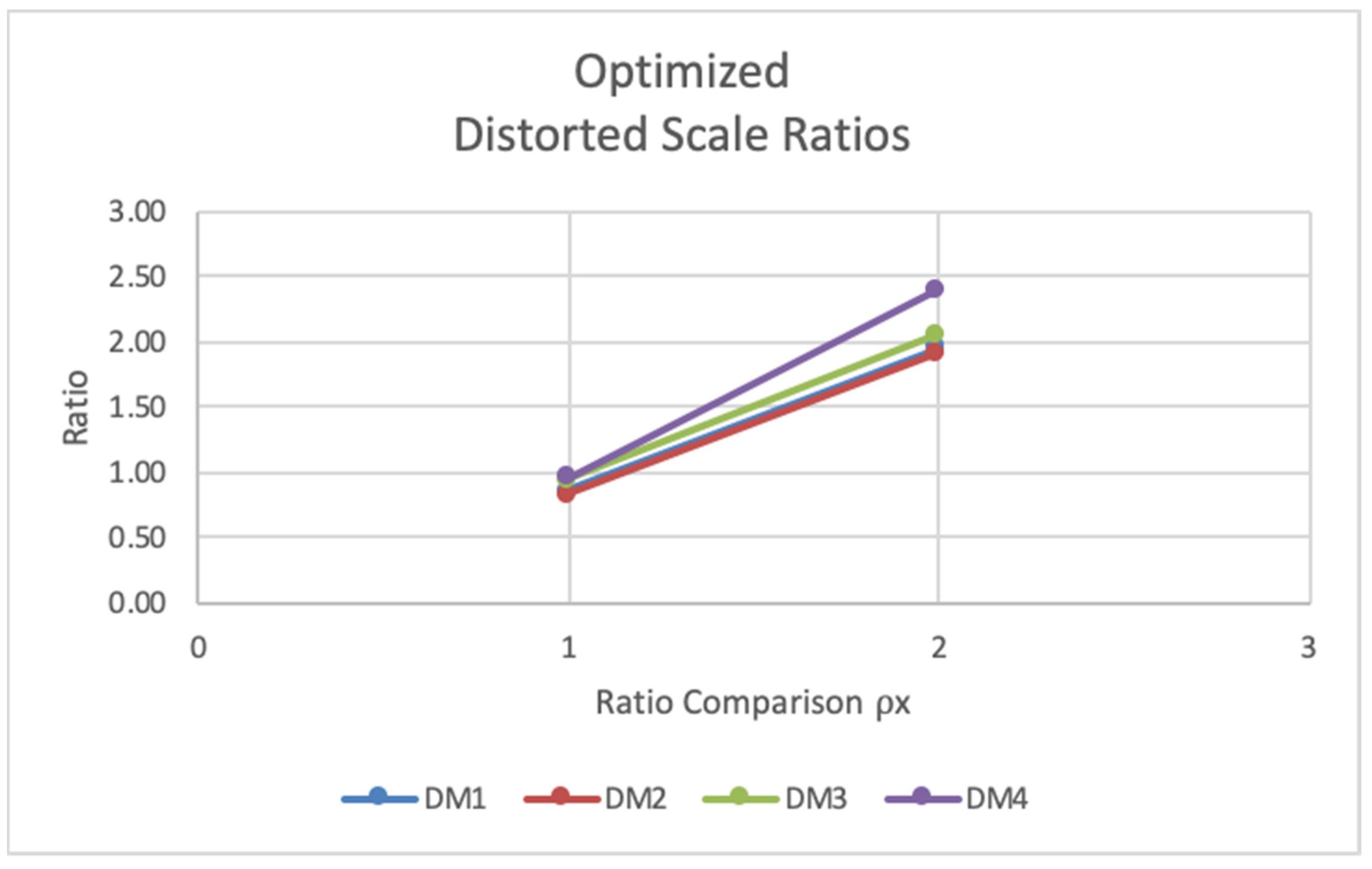Figure 5 and Figure 6 depict a scenario where scale trends display balanced distortions. There is a clear agreement between DMs in hierarchy supported by all ${\rho }_1^m<1.0$ and all ${\rho }_2^m>1.0$ in Figure 6.

Figure 5. Balanced distorted scale scores between decision makers.

Figure 6. Optimized distorted scale ratios between decision makers.

3. Optimization Method

There are two classic modes of decision making when considering a context with multiple alternatives, criteria, constraints, and objectives. If the decision-making group agrees on a set of quantifiable task variables, constraints, and objectives, then an optimum resource distribution may be obtained algorithmically. The alternative mode is to seek a satisfactory consensus distribution from group discussion [7].

Previous experiments using optimization in group decision-making processes were mainly focused on measuring the consistency between subjects (consensus) to be able to perform an optimization of a decision context given constraints or the ability of a group to concede on an appropriate and proper optimization model for their decision context [7,8,9]. Other research is focused on weighted models of interpersonal conflict in a group decision such as with the Friedkin–Johnsen model [10]. This research is uniquely different in that the optimization model intends to minimize the difference between independent value judgements of different DMs by building the constraints from the independent input of each decision maker. The constraints are built from the ratio scales that each decision maker uses in the pairwise comparisons of alternatives. The use of ratio scaling in GDM to create consistency across DMs, stronger criteria independence, and positive cross alternative anchoring forces a restructuring of the MCDM process. This restructuring is designed to identify and adjust inconsistencies and bias disparities between DMs before relative ratings are plugged into the traditional MCDM matrix shown in Table 2.

Table 2. Traditional MCDM Matrix with alternative ratings from an individual DM.

		Alternatives
Criteria	A1	A2	A3	…	Ai
C1	a11	a21	a31	…	ai1
C2	a12	a22	a32	…	ai2
C3	a13	a23	a33	…	ai3
.	.	.	.	…	.
.	.	.	.	…	.
.	.	.	.	…	.
Cj	a1j	a2j	a3j	…	aij

The optimization formulation presented here is focused on identifying where we can minimize the ratio scale disparity. This minimization must respect the boundaries of the ratio scales imposed by the DMs within the group. To accomplish this, we analyze the ratio scales across alternatives and within criteria for the group of DMs. The matrix of relative scores is shown in Table 3.

Table 3. Optimization matrix for individual criterion.

		Alternatives
Decision Maker	A1	A2	A3	…	Ai
DM1	a1j1	a2j1	a3j1	…	aij1
DM2	a1j2	a2j2	a2j2	…	aij2
DM3	a1j3	a2j3	a3j3	…	aij3
.	.	.	.	…	.
.	.	.	.	…	.
.	.	.	.	…	.
DMm	a1jm	a2jm	a3jm	…	aijm

It is important to define the critical assumptions in the decision-making process in order to rationalize the optimization formulation used in this experiment:

• Alternatives have been vetted and reduced to only the viable, best competing solutions (in this case we use $N\left(A\right)=3$ alternatives).
• Alternative criteria are rated independently against criteria requirements.
• At least 50% of DMs in the group are compatible (defined below). If not, there are very likely greater issues that need to be addressed in the process that are affecting relative ratings.

Because previous research supports the process of consistent ratio scaling, optimization can be used to reduce the ${\rho }_x^m$ ratio disparity between DMs in GDM situations with compatible DMs and situations that lack compatibility. To quantify this disparity, define:

$${\rho }_x^{max}=\underset{m\in M}{\max }{\rho }_x^m$$

(1)

and

$${\rho }_x^{min}=\underset{m\in M}{\min }{\rho }_x^m$$

(2)

For example, the difference ${\rho }_1^{max}-{\rho }_1^{min}$ is the scale distortion disparity for ${\rho }_1^{}$_. In order to reduce the total disparity and optimize the solution, we minimize the weighted sum of the ratio disparities as shown in Equation (3).

$$Minimize {{\displaystyle \sum }}_{x=1}^{N\left(A\right)-1}\left({\rho }_x^{max}-{\rho }_x^{min}\right)X_x$$

(3)

The variables in the optimization are the disparity weights $X_x$.

Consistent hierarchies amongst DMs imply consensus. In these situations, bias and dependency can still exist. Additionally, insufficient incremental scale detail can lead to inaccurate ratio comparisons. In this situation, because consensus is achieved, tighter imposed optimization constraints are appropriate, as shown in constraint Equation (4). By taking the difference between ${\rho }_1^{min}$ and ${\rho }_1^{max}$, narrow constraints are achieved. On the other hand, when DMs do not agree on hierarchies, more extreme bias exists and therefore constraints must be widened, as shown in constraint Equation (5). In this situation, to achieve the widest constraint possible, the difference of each ratio is taken from 0 (i.e., 0 – ${\rho }_2^{max}$ for the lower end and ${\rho }_1^{max}$– 0 for the upper end). Thus, the formulation has two sets of constraints, one that is used in each of these situations as described below.

Optimization for consistent hierarchies (all DMs have the same hierarchy) is subject to the following constraints:

$$\begin{gathered} \mathrm{C}1:a_{1j}^1\left({\rho }_1^{min}-{\rho }_2^{max}\right)\le a_{2j}^1{X}_1-a_{3j}^1{X}_2\le a_{1j}^1\left({\rho }_1^{max}-{\rho }_2^{min}\right) \\ \mathrm{C}2: a_{1j}^2\left({\rho }_1^{min}-{\rho }_2^{max}\right)\le a_{2j}^2{X}_1-a_{3j}^2{X}_2\le a_{1j}^2\left({\rho }_1^{max}-{\rho }_2^{min}\right) \\ ⋮ ⋮ \\ \mathrm{Cm}: a_{1j}^m\left({\rho }_1^{min}-{\rho }_2^{max}\right)\le a_{2j}^m{X}_1-a_{3j}^m{X}_2\le a_{1j}^m\left({\rho }_1^{max}-{\rho }_2^{min}\right) \end{gathered}$$

(4)

Optimization of incompatible DMs (there are at least two different hierarchies among the DMs in this criteria) is subject to the following constraints:

$$\begin{gathered} \mathrm{C}1:-a_{1j}^1{\rho }_2^{max}\le a_{2j}^1{X}_1-a_{3j}^1{X}_2\le a_{1j}^1{\rho }_1^{max} \\ \mathrm{C}2: -a_{1j}^2{\rho }_2^{max}\le a_{2j}^2{X}_1-a_{3j}^2{X}_2\le a_{1j}^2{\rho }_1^{max} \\ ⋮ ⋮ \\ \mathrm{Cm}:-a_{1j}^m{\rho }_2^{max}\le a_{2j}^m{X}_1-a_{3j}^m{X}_2\le a_{1j}^m{\rho }_1^{max} \end{gathered}$$

(5)

After the optimization is solved, the $X$ variables are used to adjust the ratios. In order to make those adjustments, we need the following definitions:

First, define a set of compatible decision makers in a criterion as those DMs that share the same hierarchy of alternative scores in that criterion. $H$ is the set of unique hierarchies represented among the ratings of all DMs for that criterion. For all of the DMs, let $h\in H$ be one of these hierarchies, $DM\left(h\right)$ be the set of DMs that indicated hierarchy $h$, and $N\left(DM\left(h\right)\right)$ be the number of compatible DMs that chose hierarchy $h$.

Now define

$$ND{M}^{*}=\underset{h\in H}{\max }N\left(DM\left(h\right)\right)$$

(6)

$$h^{*}=\underset{h\in H}{argmax}N\left(DM\left(h\right)\right)$$

(7)

Notice the following:

• $h^{*}$ is the most common hierarchy indicated by DMs for this criterion;
• $ND{M}_{}^{*}$ is the number of DMs that indicated $h_{}^{*}$ in their ratings;
• $DM\left(h_{}^{*}\right)$ is the set of DMs that indicated $h_{}^{*}$.

Next, define ${\overline{\rho }}_x\left(h\right)$ as the average of ratio $x$ across a set of compatible DMs, $DM\left(h\right)$, that chose hierarchy $h$:

$${\overline{\rho }}_x\left(h\right)={\displaystyle \sum }_{m\in DM\left(h\right)}{\rho }_x^m/N\left(DM\left(h\right)\right)$$

(8)

In order to proceed with the optimization of ratios, the following procedure is followed to leverage the information from compatible decision makers:

Case 1: If $ND{M}_{}^{*}>N\left(DM\right)/2$, then use only ratios from DMs in $DM\left(h_{}^{*}\right)$ to compute ${\overline{\rho }}_x$:

$${\overline{\rho }}_x={\overline{\rho }}_x\left(h^{*}\right)={\displaystyle \sum }_{m\in DM\left(h^{*}\right)}{\rho }_x^m/ND{M}^{*}$$

(9)

Case 2a: If $ND{M}_{}^{*}=N\left(DM\right)/2$ and there are more than two hierarchies among the DMs (i.e., there is a unique hierarchy chosen by half the DMs), then use only ratios from DMs in $DM\left(h_{}^{*}\right)$ to compute ${\overline{\rho }}_x$ (same computation as Case 1):

$${\overline{\rho }}_x={\overline{\rho }}_x\left(h^{*}\right)={\displaystyle \sum }_{m\in DM\left(h^{*}\right)}{\rho }_x^m/ND{M}^{*}$$

(10)

Case 2b: If $N_{}^{*}=N\left(DM\right)/2$ and there are only two hierarchies, each chosen by an equal number ($N\left(DM\right)/2)$ of DMs, then use all ratios in $DM$ to compute ${\overline{\rho }}_x$:

$${\overline{\rho }}_x={\displaystyle \sum }_{m\in DM}{\rho }_x^m/N\left(DM\right)$$

(11)

For example, for Case 2b, if two DMs out of four agree on a hierarchy and the other two also agree, then there are only two different hierarchies, and thus the dominant hierarchy is unclear. In this case, the ratings of all four DMs are used in ${\overline{\rho }}_x$.

Case 3: If $N_{}^{*}<N\left(DM\right)/2$ do not proceed. A majority of the DMs are not compatible.

Next, define $d_x^m$, the original distance between ${\overline{\rho }}_x$ and ${\rho }_x^m$ for DM $m$, as follows:

$$d_x^m={\overline{\rho }}_x-{\rho }_x^m \mathrm{for} x=1\dots N\left(A\right)-1, m=1\dots N\left(DM\right)$$

(12)

Next, the adjusted distance $d_x^{m, adj}$ uses the corresponding optimization solution X_x as shown in Equation (13).

$$d_x^{m, adj}=d_x^m{X}_x \mathrm{for} x=1\dots N\left(A\right)-1, m=1\dots N\left(DM\right)$$

(13)

The adjusted ratios (${\rho }_x^{m,adj}$) and ultimately adjusted alternative ratings ($a_{ij}^{m,adj}$) are then calculated using the adjusted distance ($d_x^{m, adj}$) from ${\overline{\rho }}_{x,h\left(m\right)}$ as shown in Equations (14) and (15).

$${\rho }_x^{m,adj}={\overline{\rho }}_x-d_x^{m, adj} \mathrm{for} x=1\dots N\left(A\right)-1, m=1\dots N\left(DM\right)$$

(14)

$$a_{ij}^{m,adj}=a_{ij}^m{\rho }_{i-1}^{m,adj} \mathrm{for} i=2\dots A, m=1\dots N\left(DM\right)$$

(15)

The resulting MCDM matrix for a single DM after optimizing the ratio scales for all criteria is shown in Table 4.

Table 4. Optimized MCDM matrix for DM^1.

DM1		Alternatives
Criteria	A1	A2	A3	…	Ai
C1	$a_{11}^{}$	$a_{21}^{adj}$	$a_{31}^{adj}$	…	$a_{i1}^{adj}$
C2	$a_{12}^{}$	$a_{22}^{adj}$	$a_{32}^{adj}$	…	$a_{i2}^{adj}$
C3	$a_{13}^{}$	$a_{23}^{adj}$	$a_{33}^{adj}$	…	$a_{i3}^{adj}$
.	.	.	.	…	.
.	.	.	.	…	.
.	.	.	.	…	.
Cj	$a_{1j}^{}$	$a_{2j}^{adj}$	$a_{3j}^{adj}$	…	$a_{ij}^{adj}$

4. Analysis and Discussion

As previously stated in the assumptions, test cases analyzed scenarios when at least half of the decision makers agreed on hierarchy. Twenty-one test cases were analyzed. These 21 contain each possible hierarchy combination that conflicts with hierarchy 3-1-2 (i.e., A₃ rated highest and A₂ rated lowest). The optimization toolkit of Excel Solver is used to solve for X₁ and X_2. Results are shown in Table 5.

Table 5. Original and optimized test case results for a criterion.

Case	Original Hierarchy Subgroup	A1	A2	A3	A1 Adjusted	A2 Adjusted	A3 Adjusted	Adjusted Hierarchy Subgroup
1	3-1-2	7	4	9	7	4.22	9.00	3-1-2
	3-1-2	7	6	9	7	5.77	9.00	3-1-2
	3-1-2	6	4	8	6	4.06	7.96	3-1-2
	3-1-2	4	3	5	4	2.97	5.02	3-1-2
2	3-1-2	4	3	5	4	2.74	5.20	3-1-2
	3-1-2	2	1	3	2	1.26	2.80	3-1-2
	3-1-2	4	3	5	4	2.74	5.20	3-1-2
	1-3-2	7	4	5	7	4.51	7.57	3-1-2
3	3-1-2	7	5	9	7	4.91	8.89	3-1-2
	3-1-2	8	5	10	8	5.40	10.06	3-1-2
	3-1-2	4	3	5	4	2.85	5.03	3-1-2
	1-2-3	9	8	7	9	6.78	9.75	3-1-2
4	3-1-2	6	3	9	6	3.64	9.77	3-1-2
	3-1-2	4	3	8	4	2.79	7.49	3-1-2
	3-1-2	4	3	7	4	2.79	7.00	3-1-2
	2-3-1	5	8	7	5	5.01	7.89	3-2-1
5	3-1-2	4	2	5	4	2.19	5.31	3-1-2
	3-1-2	5	3	8	5	3.03	7.71	3-1-2
	3-1-2	4	3	6	4	2.78	5.92	3-1-2
	2-1-3	4	7	3	4	5.13	4.09	2-3-1
6	3-1-2	5	3	8	5	2.93	8.25	3-1-2
	3-1-2	5	2	7	5	2.80	7.99	3-1-2
	3-1-2	4	3	8	4	2.42	7.01	3-1-2
	3-2-1	3	4	7	3	2.04	5.51	3-1-2
7	3-1-2	4	3	5	4	2.43	4.34	3-1-2
	3-1-2	5	3	7	5	2.88	5.67	3-1-2
	1-3-2	3	1	2	3	1.57	2.68	1-3-2
	1-3-2	10	6	7	10	5.77	9.05	1-3-2
8	3-1-2	3	1	5	3	1.40	4.48	3-1-2
	3-1-2	4	3	5	4	2.87	4.73	3-1-2
	1-2-3	5	4	2	5	3.74	2.72	1-2-3
	1-2-3	5	4	3	5	3.74	3.47	1-2-3
9	3-1-2	5	3	7	5	5.48	7.56	3-1-2
	3-1-2	6	3	9	6	6.37	9.34	3-1-2
	2-3-1	4	8	6	4	6.32	6.23	2-3-1
	2-3-1	3	7	6	3	5.09	5.32	3-2-1
10	3-1-2	5	3	8	5	4.13	7.08	3-1-2
	3-1-2	4	3	6	4	3.66	5.42	3-1-2
	2-1-3	4	7	3	4	6.01	3.59	2-1-3
	2-1-3	6	9	4	6	8.13	5.08	2-1-3
11	3-1-2	5	3	8	5	4.28	9.81	3-1-2
	3-1-2	5	2	7	5	4.14	9.55	3-1-2
	3-2-1	4	5	8	4	3.77	8.25	3-1-2
	3-2-1	3	4	10	3	2.86	7.20	3-1-2
12	3-1-2	5	3	6	5	3.17	6.82	3-1-2
	3-1-2	4	3	8	4	2.86	7.35	3-1-2
	1-2-3	7	6	3	7	5.42	6.35	1-3-2
	1-3-2	9	5	7	9	5.49	10.03	3-1-2
13	3-1-2	3	1	5	3	1.20	4.97	3-1-2
	3-1-2	5	3	8	5	2.66	8.05	3-1-2
	2-3-1	4	7	6	4	4.42	6.15	3-2-1
	2-1-3	6	8	4	6	5.38	5.67	1-3-2
14	3-1-2	5	2	6	5	1.89	6.20	3-1-2
	3-1-2	3	1	4	3	1.07	3.88	3-1-2
	1-3-2	8	4	7	8	3.30	8.87	3-1-2
	2-3-1	3	9	7	3	3.80	5.09	3-2-1
15	3-1-2	6	5	9	6	4.37	8.57	3-1-2
	3-1-2	5	2	6	5	2.53	6.36	3-1-2
	1-3-2	8	4	5	8	4.45	7.75	1-3-2
	2-1-3	5	6	3	5	4.58	4.78	1-3-2
16	3-1-2	7	4	10	7	4.74	9.91	3-1-2
	3-1-2	5	4	7	5	3.47	7.06	3-1-2
	1-3-2	9	3	5	9	5.92	11.59	3-1-2
	3-2-1	3	4	7	3	2.21	4.65	3-1-2
17	3-1-2	4	3	6	4	2.87	5.76	3-1-2
	3-1-2	3	2	4	3	2.09	4.18	3-1-2
	1-2-3	7	5	3	7	4.97	8.05	3-1-2
	2-3-1	2	6	5	2	2.54	3.42	3-2-1
18	3-1-2	4	3	6	4	3.20	5.72	3-1-2
	3-1-2	5	5	6	5	4.74	6.34	3-1-2
	1-2-3	7	5	4	7	5.46	6.50	1-3-2
	2-1-3	5	8	3	5	6.52	4.72	2-1-3
19	3-1-2	3	2	5	3	2.20	4.65	3-1-2
	3-1-2	6	5	8	6	4.61	8.69	3-1-2
	1-2-3	9	6	4	9	6.59	10.60	3-1-2
	3-2-1	3	5	7	3	2.84	5.26	3-1-2
20	3-1-2	4	4	5	4	3.80	5.26	3-1-2
	3-1-2	7	6	10	7	6.35	9.55	3-1-2
	2-3-1	3	8	5	3	4.40	4.29	2-3-1
	3-2-1	3	6	7	3	3.78	4.85	3-2-1
21	3-1-2	5	3	6	5	3.18	7.18	3-1-2
	3-1-2	4	3	6	4	2.86	9.05	3-1-2
	2-1-3	6	8	4	6	6.12	6.59	3-2-1
	3-2-1	4	6	7	4	4.43	7.15	3-2-1

The optimization formulation performed well when cases of bias were not extreme and consensus across all DMs was achieved, such as Case #11 shown in Figure 7, Figure 8, Figure 9 and Figure 10. Bias was considered to be extreme when at least one DM valued an alternative lowest and the other DM(s) valued the same alternative highest. In this case, DM1 and DM2 agree, and DM3 and DM4 agree on rank order of alternatives. It can be seen that the disparity in opinion is between alternative 1 and alternative 2. Recall that values of alternative criteria should be judged against criteria requirements, so there is clearly significant bias present in the evaluation between alternative 1 and alternative 2. After performing the optimization, it is shown that the bias was present in the evaluations of DM3 and DM4, and all adjusted alternative values reflect rank-order consistency (consensus) among all four DMs. It is important to note that even in situations when there is complete consensus prior to optimization, scale distortions can still exist. Therefore, weighted criteria values can skew overall alternative evaluations, necessitating adjusted scaling such as with Case #1.

Figure 7. Case #11 unbalanced distorted scales.

Figure 8. Case #11 unbalanced distorted scale ratios.

Figure 9. Case #11 adjusted distorted scales.

Figure 10. Case #11 adjusted distorted scale ratios.

In cases when bias was extreme, consensus was generally not identified after optimization. However, ratio disparities were minimized and alternative ratings and ratio scale trends were smoothed, such as in Case #18 shown in Figure 11, Figure 12, Figure 13 and Figure 14. It is shown that value disparities were significantly reduced between DMs in alternative 2 and alternative 3. So, even though consensus was not achieved in situations with extreme bias, the optimization reduced scale distortions to more accurately relate scales between DMs and provide a fairer evaluation of weighted criteria. Such situations are commensurate with decisions when group discussion may not resolve consensus.

Figure 11. Case #18 unbalanced distorted scale (extreme bias).

Figure 12. Case #18 unbalanced distorted scale ratios (extreme bias).

Figure 13. Case #18 adjusted distorted scales (extreme bias).

Figure 14. Case #18 adjusted distorted scale ratios (extreme bias).

Table 6 shows the total reduction in scale distortion disparity for each case. As shown, even in cases with extreme bias, average reduction was 54% with the tails being as high as 75%. Notice that in all cases, reductions are greater than zero for each ρ_x. Additionally, average overall reductions of cases not containing instances of extreme bias was higher at 66%. This is possibly due to the shape of the constraints in instances when consensus is stronger allowing for more confidence in bias reduction. Reductions were calculated using Equations (16) and (17).

$${\rho }_x Reduction=\frac{({\rho }_x^{max}-{\rho }_x^{min})-({\rho }_x^{max,adj}-{\rho }_x^{min,adj})}{({\rho }_x^{max}-{\rho }_x^{min})} \mathrm{for} x=1\dots N\left(A\right)$$

(16)

$$Overall Reduction=\frac{{\rho }_1 Reduction+{\rho }_2 Reduction}{2}$$

(17)

Table 6. Optimization case distortion disparity reduction.

Case	ρ1 Reduction	ρ2 Reduction	Overall Reduction
1	23%	14%	19%
2	77%	59%	68%
3 *	70%	63%	67%
4 *	64%	51%	58%
5 *	41%	39%	40%
6	87%	74%	81%
7	79%	67%	73%
8 *	40%	25%	33%
9 *	65%	56%	61%
10 *	31%	39%	35%
11	81%	59%	70%
12 *	46%	41%	44%
13 *	50%	29%	40%
14 *	66%	60%	63%
15 *	49%	47%	48%
16	92%	85%	89%
17 *	76%	73%	75%
18 *	41%	46%	44%
19 *	79%	69%	74%
20 *	69%	72%	71%
21 *	56%	57%	57%

* Denotes cases of extreme bias or disparity.

5. Conclusions

Consensus is often the measure of a sound group decision. However, consensus does not necessarily equate to balanced levels of bias across DMs, nor does it account for insufficient scale detail. Furthermore, consensus does not imply fair or balanced judgement of alternative criteria. Evidence exists to support the use of ratio scaling in pairwise comparisons of alternatives. Optimization may provide a solution to inconsistent hierarchies, unbalanced biases, and insufficient incremental scale detail. The optimization formulation and resulting test cases provided in this research support using optimization to reduce disparities between DMs to achieve stronger criteria independence and make gains toward group consensus. Further research is required to characterize different GDM contexts with varying numbers of alternatives and DMs and the viability of optimizing such scenarios. Additionally, by expanding constraints to deemed “acceptable” boundaries by the group or group facilitator, it may be possible to achieve consensus in even extremely biased cases. Finally, optimization of ratio scaling on alternative value scales opens the potential for future research and use of semiautonomous group decision-making constructs, such as a semiautonomous Delphi method. However, decision processes and support tools are only valid if they are trusted. Trust is a cornerstone in every group decision, and it must be balanced and measured as optimization decision support tools such as this are developed and institutionalized.

6. Disclaimer

The views expressed in this article are those of the authors and do not necessarily reflect the official policy or position of the Department of the U.S. Air Force, the U.S. Department of Defense, or the U.S. Government.