Abstract
Fault diagnosis is studied based on the system type, which facilitates the realization of the engineering configuration and improves the diagnosis efficiency. The fault-tolerant control method is unified based on the concept of fault compensation. According to the dynamic characteristics of the system, the method takes the boundary value of no-fault signal fluctuation as the basis for fault detection, then takes the changing intensity of the solenoid valve control signal after the fault occurs as the fault location basis. Finally, it takes the difference or ratio of the signals before and after the fault occurs as the fault estimation. For the basis of fault separation, the integral value of the fitting equation between the fault signal and time is used as the Eigenvalue of fault type separation to comprehend fault separation. A program is written in C++ and combined with MATLAB/S-Fun function to realize fault tolerance. At the same time, the dynamic model calibration and real-time fault diagnosis, and fault-tolerant control process of sensor fault diagnosis are provided, which makes it suitable for general engineering feedforward-feedback systems and has a certain suppression effect on noise. The simulation results verify that the method is not only viable and it is exact.
1. Introduction
The research purpose of this paper is based on the current configuration form of engineering system development and the limitation of the efficiency of the unified method for fault diagnosis of various systems. We intend to start from the different structures of the control system and combine the different dynamic characteristics of each system to study their faults. The diagnosis method to establish the engineering configuration method to achieve a productive system fault diagnosis. At the same time, a unified fault-tolerant method for fault diagnosis based on the compensation concept is established to facilitate engineering configuration to achieve efficient fault-tolerant control is considered. In this paper, the fault diagnosis and fault-tolerant processing of the sensor are carried out based on the feedforward-feedback control system. The sensor is an important data acquisition device in the control system and an important bridge for communication between the controller and the actuator. The normality of the sensor will directly affect the performance of the control system. Therefore, the fault diagnosis and fault-tolerant control of sensors are of great practical and application value for improving the safety and reliability of industrial systems during operation. Scholars at home and abroad have conducted extensive research on sensor fault diagnosis and fault tolerance control [1,2,3,4,5].
There are three main methods of sensor fault diagnosis. The first is fault diagnosis methods based on analytical models, such as parameter estimation methods and equivalent space methods [6,7]. The second is fault diagnosis methods based on prior knowledge, such as expert systems and neural networks [8]. The third is based on data-driven fault diagnosis methods, such as signal processing methods and multivariate statistical analysis methods [9,10,11]. In the closed-loop of the feedforward-feedback control system, the analytical model method and the prior knowledge method are hard to carry out due to the adjustment effect of the PID controller and the disturbance effect of nonlinear factors [12].
Yu Zhiwei et al. proposed a new sensor fault diagnosis technology for distributed control systems. This technology utilizes the equivalent space method to design a fault diagnosis filter bank, which can effectively reduce the fault jump amplitude caused by time lag and solve the problem of bus influence of communication lag on traditional fault diagnosis [13]. Tao Liquan et al. designed a synovial observer for aero-engine sensor fault diagnosis, which can effectively diagnose other types of faults, such as deviation and pulse faults. The synovial observer is a fault diagnosis method based on an analytical model. Compared with general linear observers, it can overcome the disturbance of nonlinear factors in the system. However, there are also disadvantages, because the aero-engine works in a high temperature and pressure environment and is interfered with by external factors such as wind and air pressure, which may cause a large deviation between the output of the observer and the actual signal, resulting in the problem of misdiagnosis [14]. Wei et al. proposed a convolutional neural network offline diagnostic method for processing time series. The method adds a shift layer after the input layer of the neural network, which avoids the loss of fault feature information due to the direct connection between the time series and convolution layer. It is worth noting that the neural network fault diagnosis method is based on the comparison between the predicted value and the actual value to achieve the fault diagnosis. The predicted value requires a large number of sample signals to train the algorithm, which is very difficult in engineering practice [15].
Fault-tolerant control is mainly divided into passive fault-tolerant control and active fault-tolerant control. Passive fault-tolerant control incorporates reliable stabilization, simultaneous stabilization, and integrity control [16]. Active fault-tolerant control incorporates control law rescheduling, control law reconfiguration design, and model tracking reconfiguration control [17]. Reference [18] proposed a fault-tolerant control scheme with a fault alarm based on the neural network by utilizing the implicit function theorem, which can perform adaptive active fault-tolerant control for nonlinear faults. Reference [19] proposed a three-loop fault-tolerant control system, which is theoretically analyzed from the perspective of the pose controller requirements of the manipulator and has high robustness to the system dealing with parameter changes. Yu Ming et al. proposed an active fault-tolerant control method based on an optimized adaptive threshold and fault reconstruction strategy. The synovial observer was used to reconstruct the fault, and then an adaptive active fault-tolerant control law was designed according to the reconstruction results. It shows that the fault-tolerant method can achieve fault detection and fault tolerance within 0.06 s [20].
At present, the fault diagnosis method based on a data-driven approach is one of the research hotspots. The output signal of the sensor has the characteristics of strong dynamics and is greatly affected by noise interference. It is difficult to implement fault diagnosis methods based on analytical models and prior knowledge. Therefore, to solve this problem, a data-driven sensor fault diagnosis and fault-tolerant control method are proposed.
2. Fault Diagnosis and Fault Tolerance Methods
2.1. Experimental Principle
The experiment was based on the complex system fault diagnosis and fault-tolerant control innovation platform of a four-capacity water tank and built a feedforward-feedback control system. By simulating and processing the sensor failure, the goal of the liquid level in the water tank stabilization at the set value even in a sensor failure environment was achieved. The complex system fault diagnosis and fault-tolerant control innovation platform are depicted in Figure 1. The block diagram of the feedforward-feedback control system is illustrated in Figure 2.
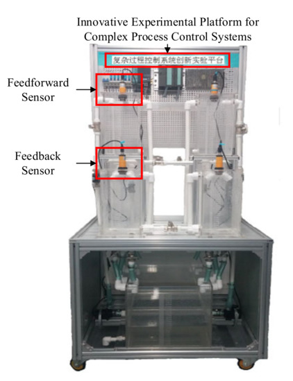
Figure 1.
The innovative platform for fault diagnosis and fault-tolerant control of complex systems.
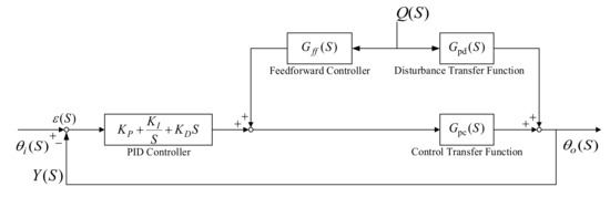
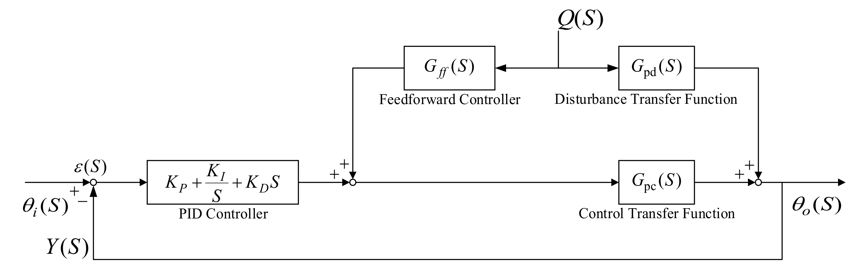
Figure 2.
Feedforward-feedback control system block diagram.
In the figure, θi(S) is the input signal; θo(S) is the output signal; Y(S) is the feedback signal; ε(S) is the deviation signal; Q(S) is the interference signal.
First, the PID controller and the feedforward controller generate the control signal of the solenoid valve based on the deviation signal and the interference signal, respectively. Then the control signal and the interference signal are canceled after passing through the control transfer function and the interference transfer function, respectively. This not only gives play to the advantages of timely feedforward correction, but also retains the advantages that feedback control can overcome various disturbances and lastly test the controlled variables.
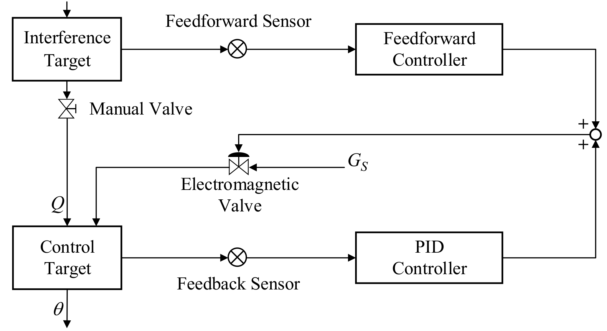
Based on the two upper and lower water tanks on the left side of the innovative platform, a feedforward-feedback control system was built, and the built-in semi-physical simulation model is shown in Figure 3.

Figure 3.
Hardware-in-the-loop simulation model.
2.1.1. Tuning PID Controller Parameters
According to the qualitative relationship between the controller parameters and the system dynamic performance and steady-state performance, the controller parameters were adjusted experimentally.
- First, set moderate PID parameters at the beginning of debugging to prevent abnormal situations such as system instability or excessive shock;
- Then a step signal is delivered and the PID parameters are set according to the overshoot of the manipulated variable and the number of oscillations.
2.1.2. Determining the Feedforward Controller Transfer Function
Adjust the opening of the manual valve to conserve the liquid level in the lower tank near the set value. For the interference channel, the opening of the manual valve is fixed, so there is a proportional relationship between the liquid level of the upper tank and its output flow, which is a first-order inertia link. For the control channel, the proportional solenoid valve is used to inversely offset the interference, which is likewise a first-order inertial link. Consequently, the transfer functions of the interference channel and the control channel are:
In the formula, Gpd(S) and Gpc(S) are the transfer functions of the interference channel and the control channel, respectively.
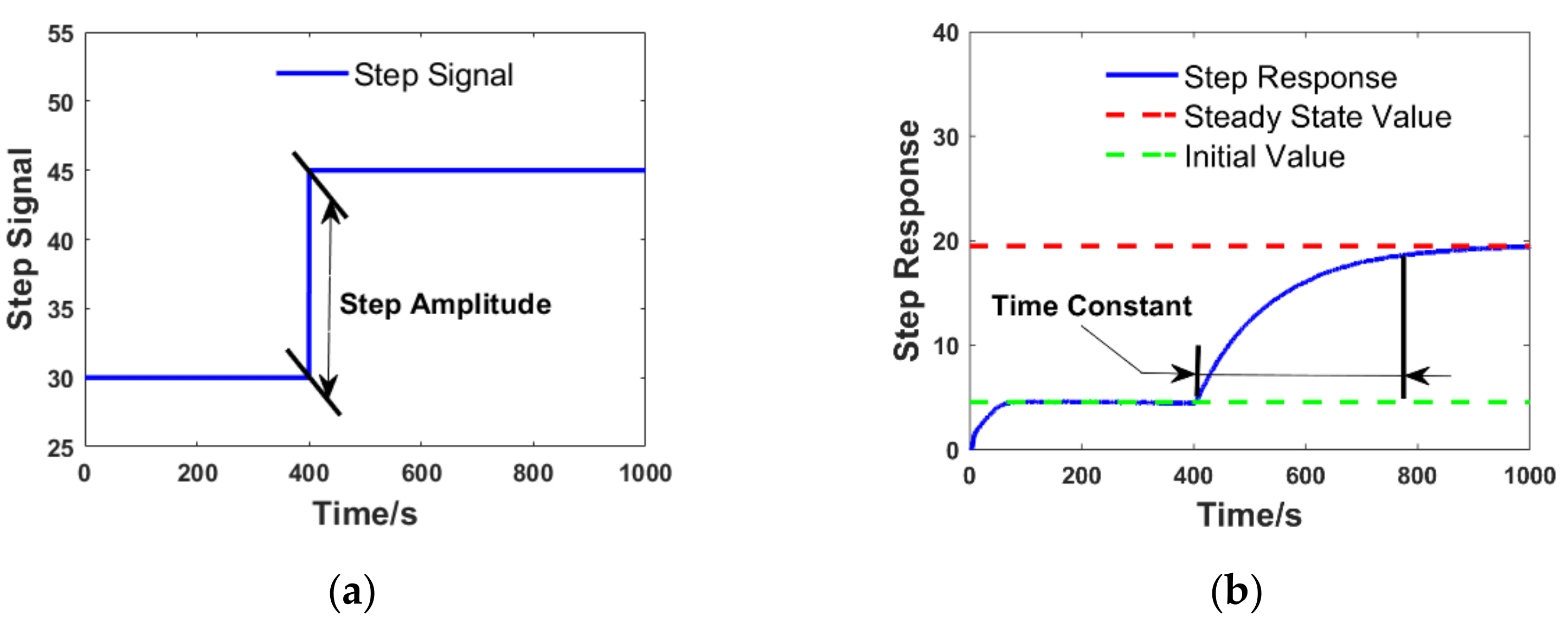
Taking the transfer function of the control channel as an example, input a step signal with a suitable amplitude to the solenoid valve, so that the lower water tank reaches a balanced state at a higher liquid level, as shown in Figure 4. The relevant parameters to determine the transfer function of the control channel based on the step response curve are:
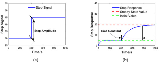
Figure 4.
The figure is a step response curve graph: (a) Step Signal; (b) Step Response Curve.
In the formula, yst represents the steady-state value of the step response curve; yin represents the initial value of the step response curve; x0 represents the amplitude of the step signal; the time constant T0 is obtained at the steady-state value of 0.632 times.
Similarly, for the transfer function of the interference channel, the step response curve of the lower tank can be obtained by increasing the liquid level of the upper tank. Subsequently, the relevant parameters of the transfer function of the interference channel are calculated according to the above method.
The transfer function of the feedforward-feedback control system illustrated in Figure 2 is:
In the formula, Gc(S) stands for PID controller transfer function. The invariance condition is applied, i.e., when Q(S) is not 0, θo(S) is 0. Substituting this relationship into the transfer function of the feedforward-feedback system, the transfer function of the feedforward controller can be derived:
The feedforward compensation device that meets the above formula can make the controlled quantity not affected by the disturbance quantity and realize the full compensation.
2.2. Fault Detection Method
Fault detection is the beginning of the fault diagnosis task. Generally speaking, the output signal of the sensor is abnormal at a certain time after the system is stable. At this time, the fault detection module detects the fault signal in time and sends an alarm signal.
When the sensor fails, its output signal will change sharply compared to the no-fault signal. Consequently, it is first required to compute the boundary value of the normal fluctuation of the non-fault signal as the basis for judging whether the sensor fails. The stack structure is used to compute the rate of change in the newly acquired signal compared to the last sampled signal in real-time. Subsequently, record the maximum rate of change in l groups of non-faulty signals, which is used to count the boundary value when the system fails:
In the formula, kM represents the change rate of the adjacent signal of the feedback sensor; kV represents the change rate of the adjacent signal of the feedforward sensor; Mt+T and Mt represent the adjacent output signal of the feedback sensor; Vt+T and Vt represent the adjacent output signal of the feedforward sensor; t and T represent the system running time and sampling period, respectively.
Taking the output signal of the feedback sensor as an example, compute the mean and standard deviation of the maximum rate of change in l groups to determine the threshold for fault detection:
In the formula, KM represents the mean value of the maximum rate of change in l groups of no-fault signals; σM represents the standard deviation of the maximum rate of change in l groups of no-fault signals; ωM represents the threshold of fault detection; vM represents the weight of the standard deviation. Use different weights to improve the accuracy of the detection.
Similarly, the fault detection threshold of the feedforward sensor is:
The fault detection method is to compare the maximum change rate of a group of signals with the threshold value. If it exceeds the threshold value range, it is established that the output signal of the sensor is inaccurate, otherwise, it is determined that the signal is not faulty.
2.3. Fault Location Method
According to the control system demonstrated in Figure 3, the output signals of the feed-forward sensor and the feedback sensor are used as the disturbance signal and the feedback signal of the system, respectively. The interference signal and feedback signal pass through the feedforward controller and the PID controller, respectively, to generate the control signal of the solenoid valve. Accordingly, the control signal can be used as the basis for the location of the fault.
When the feedback sensor has a single fault, it is equivalent to a sudden change in the liquid level of the control object. Subsequently, the solenoid valve control signal will modify sharply for reverse adjustment. The mathematical model of the feedback sensor fault location is:
In the formula, kval represents the change rate of the solenoid valve control signal; ωval represents the threshold value of the solenoid valve control signal; the tMval represents the adjustment time of the solenoid valve control signal when the feedback sensor has a single fault; the tVval represents the adjustment time of the solenoid valve control signal when the feedforward sensor has a single fault.
When a single fault of the feedforward sensor fails, the liquid level of the controlled object cannot change abruptly. Then, the rate of change in the solenoid valve control signal will not exceed the threshold. The mathematical model of the feedforward sensor fault location is:
2.4. Fault Estimation Method
The purpose of fault estimation is to confirm the strength and timing of the failure of the sensor output signal. Starting from the external characteristics of faults, this paper defined the types of faults as additive faults and multiplicative faults. The mathematical models for the two types of failures are:
In the formula, a is the deviation of the additive fault; k is the gain of the multiplicative fault; Y, Ya, and Yk are the signal values in the no-fault state, the additive fault state, and the multiplicative fault state, respectively.
Therefore, based on the mathematical model of the fault, it can be determined that the time when the fault occurs is the time corresponding to the rate of change exceeding the threshold during the fault detection process. The strength of the additive fault is the difference between the signals before and after the fault occurs, and the strength of the multiplicative fault is the ratio of the signals before and after the fault occurs. In this experiment, the deviation is called the strength of additive faults, and the gain is called the strength of multiplicative faults.
Based on the mathematical model of the fault type, determine the fault qualitative mathematical model of the feedback sensor as:
In the formula, TM represents the fault time of the feedback sensor; MTM represents the output signal of the sensor at the time of failure; MTM-T represents the sensor output signal at the moment before the failure.
Similarly, the fault intensity estimation model of the sensor output signal of the feedforward is:
2.5. Fault Isolation Method
The purpose of fault isolation is to determine whether the fault is additive or multiplicative.
2.5.1. Feedback Sensor
When different types of faults occur in a sensor, there is a deviation in the adjustment trend of the system, and the fault isolation is realized by investigating the characteristic information of the deviation. Figure 5 demonstrates the regulation trend of the system under different fault conditions.
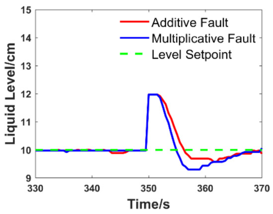
Figure 5.
System tuning trend.
Information can be drawn from the system adjustment trend chart: the signal had a sudden change in the 350th second, and after a reaction time of about two seconds, the controller started to re-adjust the system dynamically according to the fault signal until it stabilized. The system’s adjustment interval was from 2 s to 20 s after the fault occurs.
After the fault arises, the signal value in the adjustment interval of the system is fitted by the least-squares method and the time. Subsequently, to improve the sensitivity of fault characterization, the inverse function transformation is performed on the fitting equation, and the integral value of the inverse function is used as the eigenvalue of fault separation:
Taking the fault deviation (or gain) as the independent variable and the corresponding fault characteristic as the dependent variable, the characteristic equation is obtained by the univariate linear regression method:
In the formula, Ma is the characteristic equation of additive fault; Mk is the characteristic equation of multiplicative fault.
The fault estimation value is substituted into the characteristic equation to gain the corresponding Ma and Mk and then compared with the characteristic value. The feedback sensor fault separation model is:
when e1 is less than e2, it is determined that the feedback sensor has an additive failure; otherwise, it is determined that the sensor has a multiplicative failure.
2.5.2. Feedforward Sensor
Since there is no feedback loop in the feedforward channel, there is no feedback regulation of the feedforward signal after the fault occurs, but the rate of change in the faulty signal is different from the rate of change in the no-faulty signal:
In the formula, KaV is the rate of change in the output signal after an additive fault occurs; KkV is the rate of change in the output signal after a multiplicative fault occurs.
The upper water tank simulates the interference object, and the interference has no predetermined change rule. The use of the cubic polynomial fitting equation can better fit the output signal of the feedforward sensor, which perfectly reflects the linear relationship between the signal and time. The fitting equation is:
In the formula, V(t) represents the no-fault signal fitting equation; SV(t) represents the fault signal fitting equation. The estimated values of the no-fault signal and the faulty signal according to the fitting equation are:
In the formula, V(1) and V(2) represent the estimated value of the non-fault signal; SV(1) and SV(2) represent the estimated value of the fault signal; TV represents the time when the output signal of the feedforward sensor fails.
The rate of change in the additive fault value and the multiplicative fault value of the no-fault estimated value at this intensity are calculated, respectively, and then compared with the rate of change in the fault signal. The feedforward sensor fault separation model is:
when e1 is less than e2, it is determined that the feedforward sensor has an additive failure; otherwise, it is determined that the sensor has a multiplicative failure.
2.6. Fault Tolerant Control Methods
The principle of fault-tolerant control is to achieve the inverse compensation of the signal according to the fault intensity and fault type determined by the fault diagnosis result.
If there is no fault, the compensation signal is the original signal.
If an additive fault occurs, the original fault output signal will be subtracted from the fault deviation value in the fault compensation link, and then used as the feedback signal of the system. The inverse model of fault compensation is:
If a multiplicative fault occurs, the original signal will be divided by the fault gain value to switch to the feedback signal of the system, and the fault compensation inverse model is:
2.7. Online Calibration and Experimental Procedures
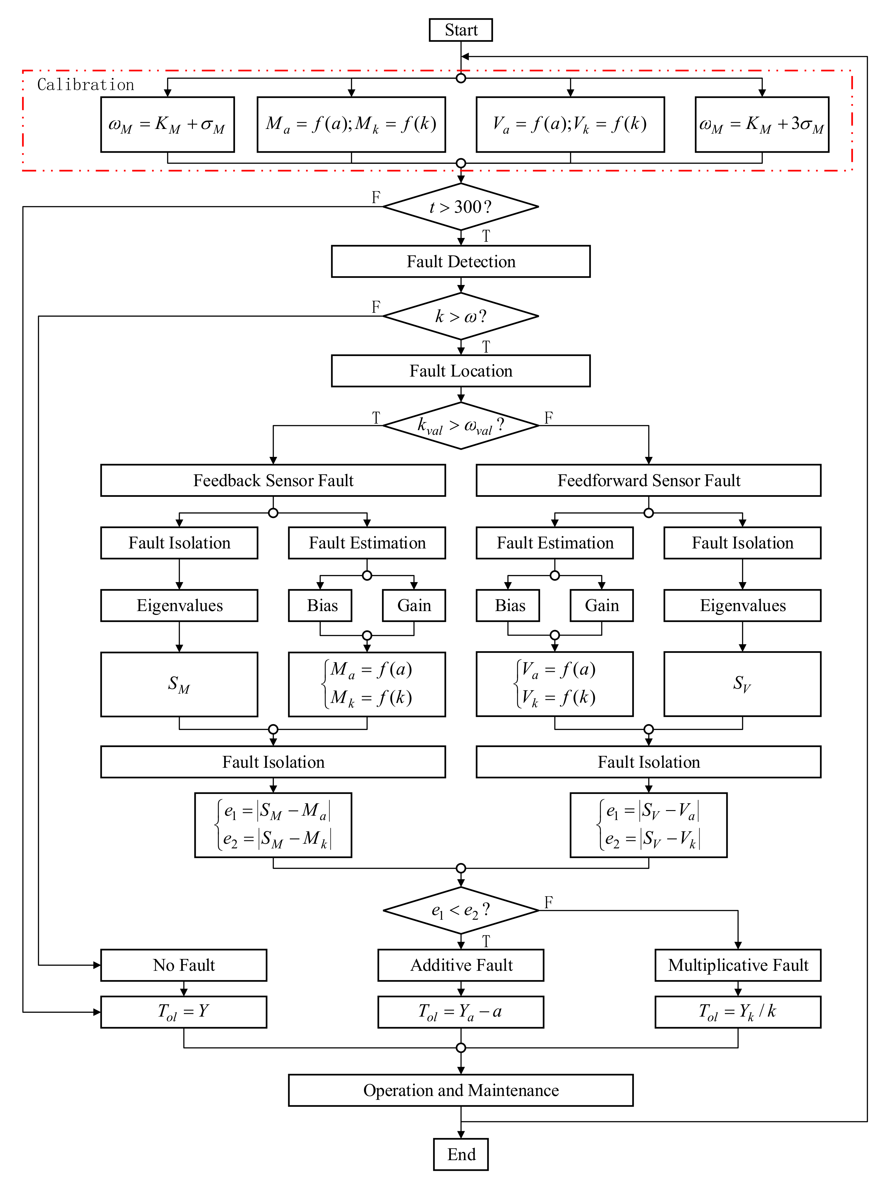
The flow of sensor fault diagnosis dynamic model calibration and real-time fault diagnosis and fault-tolerant control is demonstrated in Figure 6.
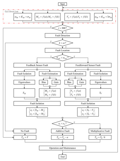
Figure 6.
Flow chart of dynamic model calibration, fault diagnosis, and fault-tolerant control.
When the system running time reached the 300th second, the fault detection procedure was started. The fault detection module processed the signal online, and if it is found that the rate of change in the signal exceeds the threshold, that is, when k is greater than ω, it is determined that the sensor is faulty. Then start the fault location procedure to determine which sensor is faulty. If kval is greater than ωval, then the feedback sensor is faulty, otherwise, the feedforward sensor is faulty. Third, determine the characteristic value and fault intensity of the faulty sensor, and characterize the fault according to the mathematical model of fault separation. Finally, the fault-tolerant compensation module inversely compensates the fault signal based on the result of fault diagnosis, to realize the correct operation of the sensor in the fault environment.
3. Simulation Verification
3.1. Test System
The innovative platform connected the OPC server to the lower computer PLC, and the MATLAB/Simulink virtual controller can regulate the liquid level of the water tank through the PID operation, combined with the configuration of the Wincc monitoring interface. Real-time monitoring and online dynamic data of Workspace in MATLAB for real-time data analysis and establishment of diagnostic and fault-tolerant models. By calling the S-Fun function to write the program, the M file was dynamically linked to the MATLAB software to realize the fault diagnosis and the verification of the fault-tolerant control method.
Combined with the hardware-in-the-loop simulation model and the experimental process, these modules were connected sequentially to the control system. After testing, there was no error in the program of each module, and the interface connection between the test modules was correct, the whole system met the requirements of function and performance and can be simulated and verified. The simulation verification model is displayed in Figure 7.
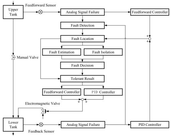
Figure 7.
Implementation with control points.
In the figure, the fault detection module was used to detect whether the sensor fails. The fault location module was used to determine which sensor is faulty. The fault estimation module was used to determine the time and intensity of the fault occurrence. The fault isolation module was used to determine the type of fault. The fault decision module was used to store the fault diagnosis results. The fault-tolerant control module was used to realize the inverse compensation of the fault signal.
3.2. Data Collection
The expected value of the control object was set to 10 cm, the system running time was 600 s, the sampling frequency was set to 2 Hz, the range of deviation was ±2 cm, and the range of gain was 0.8% to 1.2%. Faults were simulated at random time points during system operation, and then fault tolerance compensation was achieved after 50 s. The fault gradient of each set of experiments was 2%, and each sensor gathered 40 sets of fault data and 10 sets of non-fault data to determine relevant experimental parameters.
3.2.1. Determine the Threshold
Ten groups of fault-free signals were gathered, and the maximum rate of change in each group of feedforward sensor signals, the maximum rate of change in feedback sensor signals, and the maximum rate of change in control signals were calculated, and the recorded, as presented in Table 1.

Table 1.
The maximum rate of change in the no-fault signal.
The mean and standard deviation of 10 groups of data were computed and the thresholds of the sensor and solenoid valve control signals were determined. The results are shown in Table 2.
Table 2.
Threshold-related parameters.
Lastly, the threshold value of the feedforward sensor signal was 0.031, the threshold value of the feedback sensor signal was 0.036, and the change rate of the solenoid valve control signal was 0.068.
3.2.2. Determine the Characteristic Equation
The characteristic equation of the feedback sensor fault data was determined, according to the fault separation algorithm. The eigenvalues of various types of fault signals are shown in Table 3, Table 4, Table 5 and Table 6. The characteristic equations determined are shown in Table 7. (Note: Call the MATLAB/Ployfit function for data fitting).
Table 3.
Eigenvalues of a > 0.
Table 4.
Eigenvalues of a < 0.
Table 5.
Eigenvalues of k > 1.
Table 6.
Eigenvalues of k < 1.
Table 7.
Eigenvalue fitting equation.
3.3. Failure Detection Algorithm Verification
The obtained fault signal was identified according to the fault detection algorithm to determine the detection accuracy of the algorithm.
Table 8 and Table 9 exhibit the detection results of some faults. (Note: ‘0’ means no-fault identified; ‘1’ means fault identified)
Table 8.
Additive fault detection results.
Table 9.
Multiplicative fault detection results.
When the deviation range was outside ±0.2 and the gain range was outside 0.92 to 1.02, the fault detection algorithm can detect whether the sensor fails, according to the fault detection results.
The sensor’s fault signal was re-collected for fault location, fault estimation, fault separation, and fault-tolerant control algorithm verification, according to the fault detection results. The sample data were fault signals with deviations of ±5 mm and gains of 1.05 and 0.95. Figure 8 and Figure 9 show some data before and after the failure. Figure 10 and Figure 11 show the fault detection results.
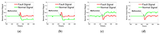
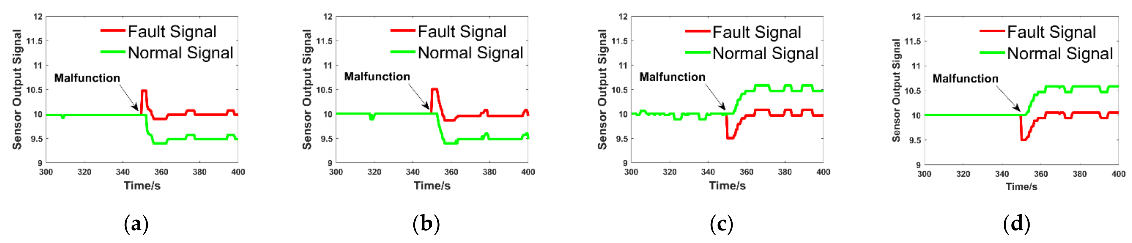
Figure 8.
Feedback sensor data: (a) Fault data with a deviation of 0.5; (b) Fault data with a gain of 1.05; (c) Fault data with a deviation of −0.5; (d) Fault data with a gain of 0.95.
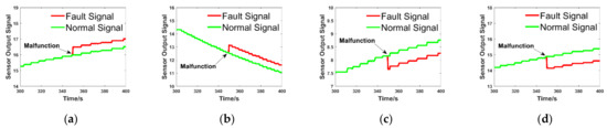
Figure 9.
Feedforward sensor data: (a) Fault data with a deviation of 0.5; (b) Fault data with a gain of 1.05; (c) Fault data with a deviation of −0.5; (d) Fault data with a gain of 0.95.
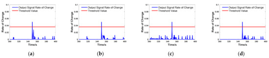
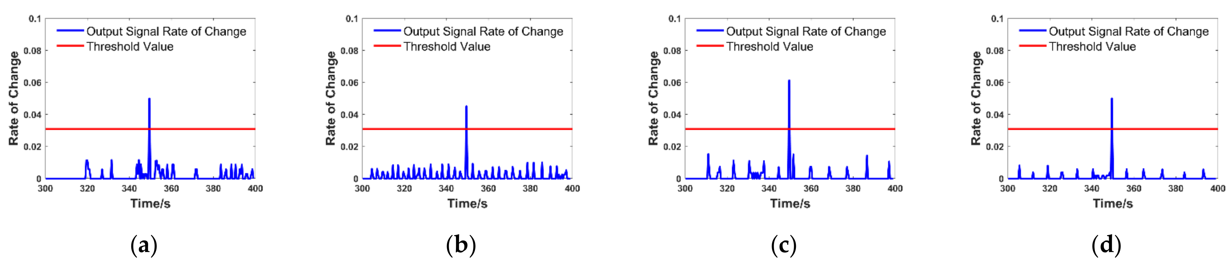
Figure 10.
Feedback sensor fault detection results: (a) Fault data with a deviation of 0.5; (b) Fault data with a gain of 1.05; (c) Fault data with a deviation of −0.5; (d) Fault data with a gain of 0.95.
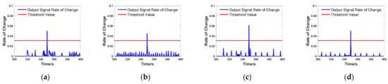
Figure 11.
Feedforward sensor fault detection results: (a) Fault data with a deviation of 0.5; (b) Fault data with a gain of 1.05; (c) Fault data with a deviation of −0.5; (d) Fault data with a gain of 0.95.
According to the fault detection result, the rate of change in the sensor output signal exceeded the threshold, so it can be calculated that both the feedforward sensor and the feedback sensor are faulty.
3.4. Failure Location Algorithm Verification
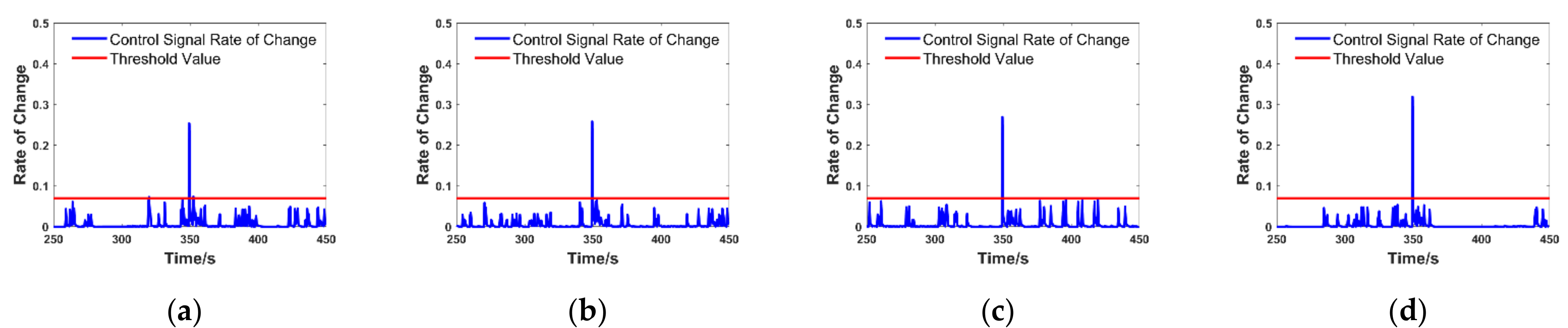
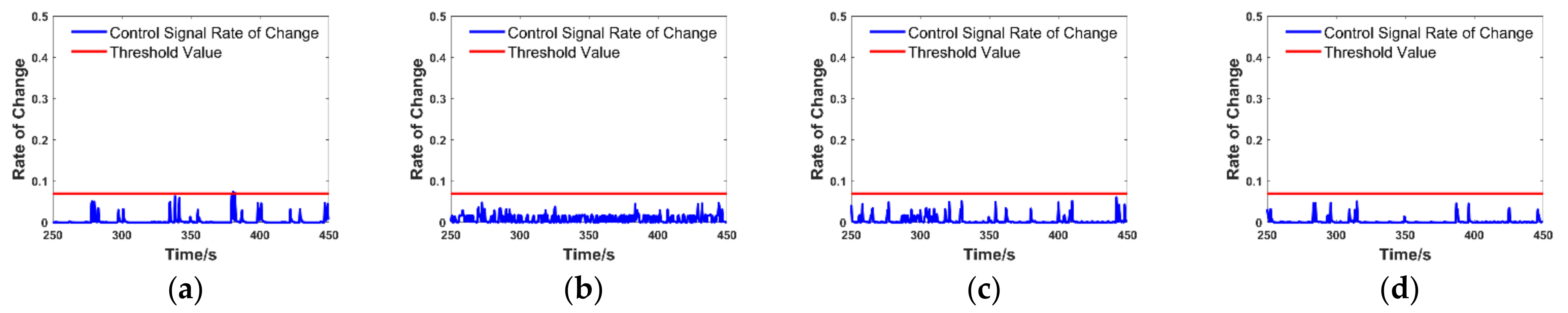
Figure 12 and Figure 13 are the change rates of the solenoid valve control signals corresponding to the above experimental data.
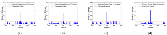
Figure 12.
The rate of change in the solenoid valve control signal when the feedback sensor is a single fault: (a) The rate of change in the control signal when the deviation was 0.5; (b) The rate of change in the control signal when the gain was 1.05; (c) The rate of change in the control signal when the deviation was −0.5; (d) The rate of change in the control signal when the gain was 0.95.
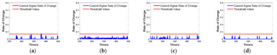
Figure 13.
The rate of change in the solenoid valve control signal when the feedforward sensor is a single fault: (a) The rate of change in the control signal when the deviation was 0.5; (b) The rate of change in the control signal when the gain was 1.05; (c) The rate of change in the control signal when the deviation was −0.5; (d) The rate of change in the control signal when the gain was 0.95.
According to the fault location results, it can be concluded that when the rate of change in the control signal exceeded the threshold, it was determined that the feedback sensor was faulty. Otherwise, it was determined that the feedforward sensor was faulty.
3.5. Fault Estimation Algorithm Verification
According to the fault detection result, the fault occurrence time of the feedforward sensor and the feedback sensor was the 350th second. Taking the experimental data of Figure 8a as an example, according to the estimation model of the fault intensity, the signal may have an additive fault with a deviation of 0.5 or a multiplicative fault with a gain of 1.0501. Similarly, the strength estimation results of other fault signals are shown in Table 10.
Table 10.
Fault estimation results.
3.6. Fault Isolation Algorithm Verification
The fitting interval of the fault signal of the feedback sensor was 2 s to 10 s after the fault occurred. The fitting interval of the fault signal of the feedforward sensor was 50 s before and after the fault occurred. Table 11 shows the feedback sensor fault separation results. Table 12 shows the fault separation results of the feed-forward sensor.
Table 11.
Feedback sensor diagnostic results.
Table 12.
Feedforward sensor diagnostic results.
The fault diagnosis results were consistent with the experimental data and satisfied the conditional requirements of fault-tolerant control.
3.7. Fault Tolerant Control Algorithm Verification
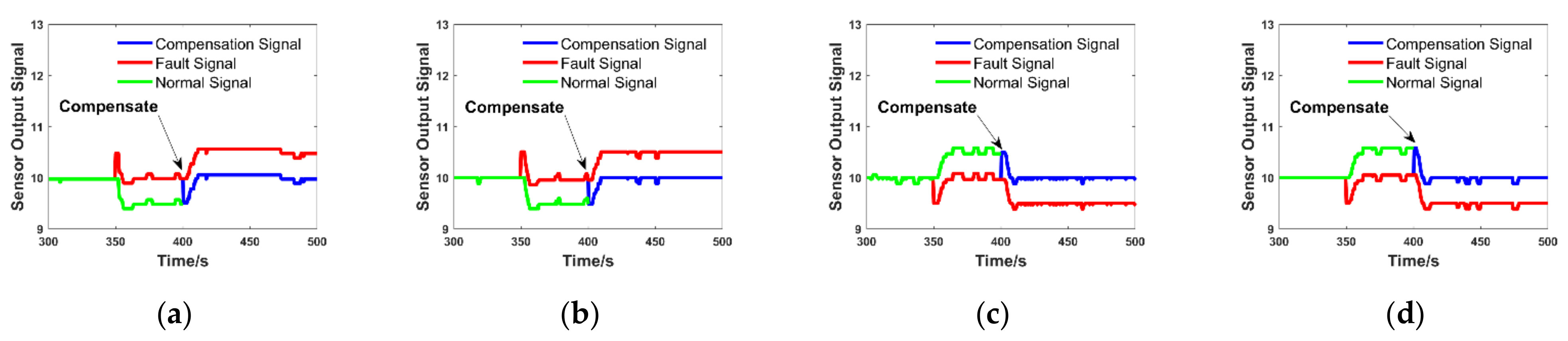
To sufficiently reflect the fault-tolerant process, this experiment was set to start the fault-tolerant control program 50 s after the fault occurred, and the compensation results are shown in Figure 14 and Figure 15.
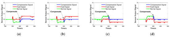
Figure 14.
Feedback sensor fault compensation results: (a) Compensation signal with a deviation of 0.5; (b) Compensation signal with a gain of 1.05; (c) Compensation signal with a deviation of −0.5; (d) Compensation signal with a gain of 0.95.
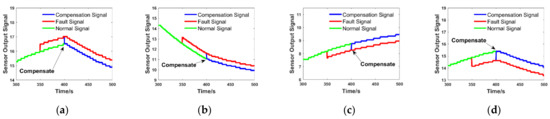
Figure 15.
Feedforward sensor fault compensation results: (a) Compensation signal with a deviation of 0.5; (b) Compensation signal with a gain of 1.05; (c) Compensation signal with a deviation of −0.5; (d) Compensation signal with a gain of 0.95.
The no-fault signal stabilized around the setpoint before the feedback sensor failed. At the 350th second, a fault occurred, and the system adjusted the liquid level based on the fault signal, so that the no-fault signal deviated from the set value, while the fault signal stabilized around the set value. At the 400th second, the fault-tolerant control program was started, and the compensation signal was inversely compensated based on the fault signal, which coincided with the no-fault signal. Finally, the system proceeded to modify the liquid level based on the compensation signal so that the compensation signal was stable near the set value.
Before the feedforward sensor failed, the no-fault signal accurately displayed the liquid level of the upper tank. At the 350th second a fault occurred, and the fault signal deviated from the actual liquid level. In the 400th second, the fault-tolerant control program was started, and the compensation signal was inversely compensated based on the fault signal, which coincided with the no-fault signal, indicating that the compensation signal accurately displayed the liquid level of the upper water tank.
4. Discussion
In order to reflect the novelty and superiority of the fault diagnosis and fault-tolerant control method proposed in this paper, the accuracy of fault diagnosis, fault-tolerant control accuracy, universality, and anti-interference were compared with some references. The comparison results are shown in Table 13. (Ⅰ: Inferior; Ⅱ: Medium; Ⅲ: Higher)
Table 13.
Research comparison.
In this experiment, after further processing the fault signal, it was determined that the feedback sensor fault detection dead zone was 2%, the fault location accuracy was 100%, the maximum error of fault estimation was less than 1%, and the fault separation dead zone was 0%. It was determined that the fault detection dead zone of the feedforward sensor was 2%, the fault location accuracy was 100%, the maximum error of fault estimation was less than 1.5%, and the fault separation dead zone was 0%. In summary, the fault diagnosis accuracy of this experiment was about 98.5%, and the deviation between the compensation signal and the normal signal was less than 0.05%.
Compared with the literature in Table 13, the novelty of this method is that it can determine the type and intensity of faults, which are not covered in other articles. The superiority of this paper is that it has higher accuracy in fault diagnosis and fault-tolerant control and higher anti-noise interference ability. More importantly, the fault handling method has excellent universality.
Combined with the above fault handling results, the fault diagnosis method proposed in this paper can fully mine the fault information even for weak faults, such as the time when the fault occurred, the intensity of the fault, and the type of the fault. The fault-tolerant control module can realize the accurate inverse compensation of the fault signal according to the fault diagnosis result, to achieve the goal that the sensor can still output a fault-free signal in the fault state, and ensure the normal operation of the control system, which is beneficial to improving the safety and reliability of the industrial system.
Although the fault diagnosis algorithm still has high diagnostic accuracy even for some weak faults, due to the influence of system noise and environmental noise on the fault detection accuracy, the phenomenon of feedback sensor compensation confusion will appear in the empirical verification link. There are two solutions to this problem. The first idea is to merge the stacking concept with the dynamic window residual sum method. The maximal window residual of each group of signals and the threshold used to determine the fault detection can effectively reduce the false alarm rate of the fault. The second idea is to utilize a slow flow device to reduce the fluctuation of the liquid level from a practical point of view, thereby reducing the impact of environmental noise.
In addition, complex control systems will likewise have multiple faults, and these faults will show propagation, that is, abnormal equipment can not only cause sub-equipment to fail but also other related equipment to fail. For example, when the actuator fails, it may also cause a sudden change in the sensor, which can lead to misdiagnosis. Accordingly, for the problem of multiple faults and the non-single mapping relationship between faults and causes, the characteristic information of distinct faults should be sufficiently excavated to form a complete set of fault diagnosis methods. This method not only has highly important educational value but also has very realistic application value [22].
The ultimate goal of theoretical research is to apply it to engineering practice. To understand the real-time fault diagnosis and fault-tolerant control of sensors using algorithms in engineering applications, the MATLAB/S-Fun function was used. This is because MATLAB/Simulink is an important modeling and simulation tool for studying dynamic systems. Its powerful graphical modeling capabilities are generally used in the control field, particularly the S-Fun function it provides. We can utilize C, MATLAB, and C++ by ourselves and other languages to write modules to extend the functionality of Simulink. At present, the fault processing method is still in the theoretical research stage, and many experiments are needed to further optimize the fault diagnosis and fault-tolerant control algorithm. Therefore, the sensor fault diagnosis and fault-tolerant control algorithm based on the feedforward-feedback control system currently designed will be verified in the field of chemical process, so that more noise interference factors can be considered, and the fault processing algorithm can be further optimized.
5. Conclusions
Based on the current configuration forms of engineering system development and the limitations of the efficiency of unified methods for fault diagnosis of various systems, this paper summarized related fault diagnosis and fault-tolerant control methods. Combined with the research results of contemporary fault diagnosis and fault-tolerant control theory and engineering application, a real-time diagnosis and fault-tolerant control scheme based on the data-driven feedforward-feedback control system for single sensor fault was proposed. Given the complex nonlinear problems of the actual industrial system, this scheme considered fault diagnosis by using the data generated during the operation of the system. The fault characteristic information was extracted by analyzing the real-time data during the operation of the system, and a mathematical model of fault detection, fault location, fault estimation, fault separation, and fault-tolerant control was established based on this characteristic information. Through a large number of simulation experiments, it was proven that the fault diagnosis method has the advantages of small calculations, strong real-time performance, and high anti-interference ability. Most importantly, it can effectively overcome the problems of low diagnostic efficiency caused by the difficulty of modeling the system and the lack of empirical knowledge in traditional fault diagnosis methods.
The main contributions of this paper are: First, based on the structure of the control system, the ideas of efficient fault diagnosis and unified and efficient fault-tolerant control based on compensation were studied, respectively, which is convenient for engineering configuration. The second is based on the dynamic characteristics of the system and real-time data drive, the proposed feedforward-feedback control system sensor fault diagnosis, and the fault-tolerant control method, which improves the accuracy of fault diagnosis and the performance of fault-tolerant control. Third, the dynamic model calibration and real-time fault diagnosis, and fault-tolerant control process of sensor fault diagnosis are given, which makes the method suitable for general engineering feedforward-feedback control system, and has a certain degree of restraining effect on the noise of engineering system.
At present, there is still a gap between the research content of this paper and the above goals, and only the fault handling task of one type of equipment in the feedforward-feedback control system was completed. In the following scientific research tasks, we will continue to study the fault handling methods of other equipment and other systems and strive to establish an effective system fault diagnosis engineering configuration method and fault-tolerant control method.
Author Contributions
Conceptualization, W.N.; methodology, W.N., Q.Z.; software, Q.Z.; validation, W.N., Q.Z.; formal analysis, W.N., Q.Z., Y.G., Z.W.; investigation, Q.Z., Y.G., S.G.; resources, Z.W.; data curation, Q.Z.; writing—original draft preparation, Q.Z.; writing—review and editing, W.N.; visualization, Q.Z.; supervision, W.N., S.G.; project administration, W.N.; funding acquisition, W.N. All authors have read and agreed to the published version of the manuscript.
Funding
This research is supported by the Project of Public Welfare Technology Application Industry Field of the Zhejiang Natural Science Foundation Committee (LGG20F 030005).
Data Availability Statement
The data presented in this study are available on request from the corresponding author. The data are not publicly available due to [privacy].
Conflicts of Interest
The authors declare no conflict of interest.
References
- Zhong, M.; Xue, T. A survey on model-based fault diagnosis for linear discrete time-varying systems. Neurocomputing 2018, 306, 51–60. [Google Scholar] [CrossRef]
- Wang, X.Q.; Wang, Z.; Xu, Z.X. Comprehensive diagnosis and tolerance strategies for electrical faults and sensor faults in dual three-phase drives. IEEE Trans. Power Electron. 2019, 34, 6669–6684. [Google Scholar] [CrossRef]
- Zhang, Z.L.; Xiao, B.X. Sensor fault diagnosis and fault-tolerant control for forklift based on sliding mode theory. IEEE Access 2020, 8, 84858–84866. [Google Scholar] [CrossRef]
- Cartocci, N.; Napolitano, M.R.; Costante, G.; Valigi, P.; Fravolini, M.L. Aircraft robust data-driven multiple sensor fault diagnosis based on optimality criteria. Mech. Syst. Signal Process. 2022, 170, 108668. [Google Scholar] [CrossRef]
- Tan, Q.; Mu, X.W.; Fu, M.; Yuan, H.Y.; Sun, J.H.; Liang, G.H.; Sun, L. A new sensor fault diagnosis method for gas leakage monitoring based on the naive Bayes and probabilistic neural network classifier. Measurement 2022, 194, 111037. [Google Scholar] [CrossRef]
- Qian, Y.J.; Kan, Z.; Liu, X.; Luo, L. Simulation Research on Sensitivity of Ring Electrostatic Sensor by Nonparametric Estimation Method. Sens. Microsyst. 2021, 40, 37–40. [Google Scholar]
- Enciso, L.; Noack, M.; Reger, J.; Pérez-Zuñiga, G. Modulating Function-Based Fault Diagnosis Using the Parity Space Method. IFAC Pap. Online 2021, 54, 268–273. [Google Scholar] [CrossRef]
- Pan, X.W.; Zhang, F.S.; Lu, C. Design of Fault Diagnosis Expert System Based on Fault Tree. Coal Min. Mach. 2021, 42, 174–176. [Google Scholar]
- Wu, G.Q.; Tao, Y.C.; Zeng, X. Data-driven transmission sensor fault diagnosis method. Journal of Tongji University. 2021, 49, 272–279. [Google Scholar]
- Zhou, G.L.; Jiang, Y.Q.; Lu, J.X.; Mei, G.M. Comparison of Vibration Signal Processing Methods for Fault Diagnosis Model Based on Convolutional Neural Network. Chin. Sci. Pap. 2020, 15, 729–734. [Google Scholar]
- Liu, Y.Y.; Li, X.Y.; Zhang, G.R.; Du, W.Q.; Cai, B.B. Sensor fault detection in papermaking wastewater treatment process based on multivariate statistical analysis. Zhonghua Pap. 2017, 38, 41–48. [Google Scholar]
- Zhou, D.H.; Liu, Y.; He, X. Review on Fault Diagnosis Techniques for Closed-loop Systems. Acta Autom. Sin. 2013, 39, 1933–1943. [Google Scholar] [CrossRef]
- Yu, Z.W.; Guo, Y.Q. Sensor Fault Diagnosis Technology of Turboshaft Engine Distributed Control System. Propuls. Technol. 2022, 43, 318–325. [Google Scholar]
- Tao, L.Q.; Ma, Z.; Wang, W.; Zhang, Z.; Liu, C. A comparative study of sensor fault diagnosis methods based on sliding mode observer and neural network. Meas. Control. Technol. 2020, 39, 21–27. [Google Scholar]
- Wei, R.N.; Jiang, J.; Xu, H.Y.; Zhang, D.M. Novel topology convolutional neural network fault diagnosis for aircraft actuators and their sensors. Trans. Inst. Meas. Control 2021, 43, 2551–2566. [Google Scholar] [CrossRef]
- Zhou, D.H.; Ding, X. Fault Tolerant Control Theory and Its Application. Acta Autom. Sin. 2000, 26, 788–797. [Google Scholar]
- Zhang, W.C.; Li, Q. Stable weighted multiple models adaptive control: Discrete-time stochastic plant. Int. J. Adapt. Control Signal Process. 2013, 27, 562–581. [Google Scholar] [CrossRef]
- Shen, Q.; Jiang, B.; Shi, P.; Lim, C.-C. Novel neural networks-based fault-tolerant control scheme with fault alarm. IEEE Trans. Cybern. 2014, 44, 2190–2201. [Google Scholar] [CrossRef]
- Yang, P. Research on Adaptive Fault-Tolerant Control Technology of Rigid Satellite Attitude Control System under Actuator Failure. Master Thesis, Nanjing University of Posts and Telecommunications, Nanjing, China, 2019. [Google Scholar]
- Yu, M.; LI, W.L.; Lan, D. Sensor Fault Detection and Active Fault Tolerant Control of Nonlinear Electromechanical Systems Based on Optimal Adaptive Threshold. J. Instrum. 2022, 43, 1–11. [Google Scholar]
- Wen, J.B.; Zhao, H.Y.; Liu, Z.N.; Bao, H. Sensor Fault Diagnosis and Fault Tolerance Processing Based on Improved Neural Network. Sens. Microsyst. 2019, 38, 132–134, 138. [Google Scholar]
- Peng, K.X.; Ma, L.; Zhang, K. Review of Quality-related Fault Detection and Diagnosis Techniques for Complex Industrial Processes. Acta Autom. Sin. 2017, 43, 349–365. [Google Scholar]


Publisher’s Note: MDPI stays neutral with regard to jurisdictional claims in published maps and institutional affiliations. |
© 2022 by the authors. Licensee MDPI, Basel, Switzerland. This article is an open access article distributed under the terms and conditions of the Creative Commons Attribution (CC BY) license (https://creativecommons.org/licenses/by/4.0/).