Article

Combined Grey Wolf Optimizer Algorithm and Corrected Gaussian Diffusion Model in Source Term Estimation

Jiangsu Key Laboratory of Hazardous Chemicals Safety and Control, College of Safety Science and Engineering, Nanjing Tech University, Nanjing 211816, China
*
Author to whom correspondence should be addressed.
Processes 2022, 10(7), 1238; https://doi.org/10.3390/pr10071238
Submission received: 24 May 2022 / Revised: 16 June 2022 / Accepted: 18 June 2022 / Published: 22 June 2022

Abstract

:
It is extremely critical for an emergency response to quickly and accurately use source term estimation (STE) in the event of hazardous gas leakage. To determine the appropriate algorithm, four swarm intelligence optimization (SIO) algorithms including Gray Wolf optimizer (GWO), particle swarm optimization (PSO), genetic algorithm (GA) and ant colony optimization (ACO) are selected to be applied in STE. After calculation, all four algorithms can obtain leak source parameters. Among them, GWO and GA have similar computational efficiency, while ACO is computationally inefficient. Compared with GWO, GA and PSO, ACO requires larger population and more iterations to ensure accuracy of source parameters. Most notably, the convergence factor of GWO is self-adaptive, which is in favor of obtaining accurate results with lower population and iterations. On this basis, combination of GWO and a modified Gaussian diffusion model with surface correction factor is used to estimate the emission source term in this work. The calculation results demonstrate that the corrected Gaussian plume model can improve the accuracy of STE, which is promising for application in emergency warning and safety monitoring.

1. Introduction

In recent years, there have been frequent public safety accidents caused by hazardous gas leakages or emissions in the process of industrial production, leading to serious harm to human safety and the ecological environment. Therefore, it puts forward a higher requirement for source term estimation (STE) methods. The main methods for locating source terms are stochastic probability method based on Bayes inference, inverse Lagrangian stochastic models and optimization methods [1,2].
On the one hand, various algorithmic methods were developed to improve the accuracy and efficiency of STE. For example, Sohn et al. combined Bayesian inference and stochastic Monte Carlo methods (BMC) in probabilistic statistics for estimating leak source parameters [3,4,5]. However, the computational efficiency of the BMC method is low [6]. Subsequently, Markov chain Monte Carlo sampling method (MCMC) has received attention, which is applied in solving multi-source estimation [7,8,9,10,11,12,13,14]. Methods based on probability and statistics like MCMC require a lot of prior data. Such methods are not applicable in emergency situations where prior data is insufficient and time is limited.
Therefore, it is a better choice to use optimization algorithm to trace the source of leakage in emergency situations. Singh et al. [15,16] employed the least-squares method for emission source estimation. Bieringer et al. [17] combined a quasi-Newtonian method, the Broyden–Fletcher–Goldfarb–Shanno (BFGS) algorithm, with a simple Gaussian diffusion model to refine an initial guess of source parameters obtained from an inverse SCIPUFF run. Classical algorithms, such as Newton’s method and least square method, are fast in calculation, but they are very dependent on initial values and tend to fall into local extremums. Meta-heuristic algorithms have global search capability and are often used in STE of source parameters. Commonly used heuristic optimization algorithms in source item identification studies include genetic algorithm (GA), simulated annealing (SA), particle swarm optimization (PSO), etc. GA transforms the optimization process into a process similar to the crossover and mutation of chromosomal genes in biological evolution, and can quickly obtain good optimization results [18]. SA is a widely used optimization algorithm that can effectively solve local optimal solution problems [19]. PSO was inspired by bird predation which was often used to deal with complex nonlinear problems [20]. ACO is an intelligent optimization algorithm with better superiority in discrete optimization problems [21]. Wang [22] used a hybrid GA to reverse the source term and proposed composite cost functions named WSD to improve the estimation accuracy. Wang et al. [23] proposed a hybrid strategy to improve the performance of STE by combining PSO, GA and SA, but such strategy makes the computing time slightly longer. Recently, SIO has received attention in several fields, especially in STE. Ma et al. introduced the firefly algorithm (FA) to track emission sources., and proposed an active firefly algorithm (AFA) to improve the accuracy and efficiency of STE [24,25]. However, each optimization algorithm has their certain serviceability, leading to some limitations. For example, GA has poor local search capability and PSO is prone to fall into local extremes. Therefore, it is necessary to find an algorithm that combines excellent local optimization and global optimization ability to improve STE.
On the other hand, the diffusion model has a significant impact on the accuracy of STE. Numerous studies improve the accuracy of STE by enhancing the accuracy of diffusion models. [26] proposed a diffusion model based on radial basis function neural network and Gaussian model (Gaussian-RBF network) to improve the performance of STE. Wu et al. [27] combined Bayesian inference and CFD model to propose an effective SET model. Allen, Haupt and Young [28] added the more complex the Second-Order Closure Integrated Puff (SCIPUFF) model to the GA-based STE model and demonstrated its applicability. However, complex diffusion models reduce the estimation efficiency, and simple models are difficult to apply to various scenarios. Therefore, it is necessary to modify the simple model to suit more complex environments.
In this study, a novel swarm intelligence optimization algorithm, GWO, is combined with a modified Gaussian diffusion model to improve the performance of STE. Different methods were used to compare with GWO. In order to study the applicability of GWO to STE inverse problem, the influence of different factors on GWO in estimating source term have been tested. The results show that GWO can estimate the source term quickly and reliably, and has great application prospects in early warning. In addition, a modified Gaussian diffusion model is introduced in STE by adding a terrain correction parameter, which shows strong applicability in different terrains by case validation.

2. Models and Methods

2.1. STE Model Based on Optimization Algorithm

The principle of the STE model based on the optimization algorithm is to transform the problem of estimating the source parameters into an optimization problem of finding the minimum value. In this paper, GWO algorithm is mainly used to solve the objective function. The basic form of the objective function is shown in Equation (1).
m i n f o b j = i = 1 N C o b s i C p r e i 2
where C o b s i is the concentration measured by the sensor at the position i;   C p r e i is the concentration predicted by the forward dispersion model; N is the number of the measurement;   m i n f o b j is the object function, which represents the error between measurement and prediction.
Gaussian plume model is widely used in STE due to its ease to use, high computational efficiency, and high accuracy. In order to compare and contrast with the previous work, the Gaussian plume model is used as the forward diffusion model in this paper when discussing the feasibility of the algorithm. The basic Gaussian plume model is represented as follows:
C x , y , z = Q 2 π u σ y σ z e x p 1 2 y 2 σ y 2 e x p 1 2 z H σ z 2 + e x p 1 2 z + H σ z 2
where C(x, y, z) is the gas concentration at position (x, y, z), g/m3; u is the wind speed, m/s; Q is the emission source strength, g/s; H is the height of the plume, m; σ y and σ z are the distance deviation coefficients in crosswind and vertical direction, which are determined by the recommended formulas [29]. Atmospheric stability is classified with Pasquill’s stability category.

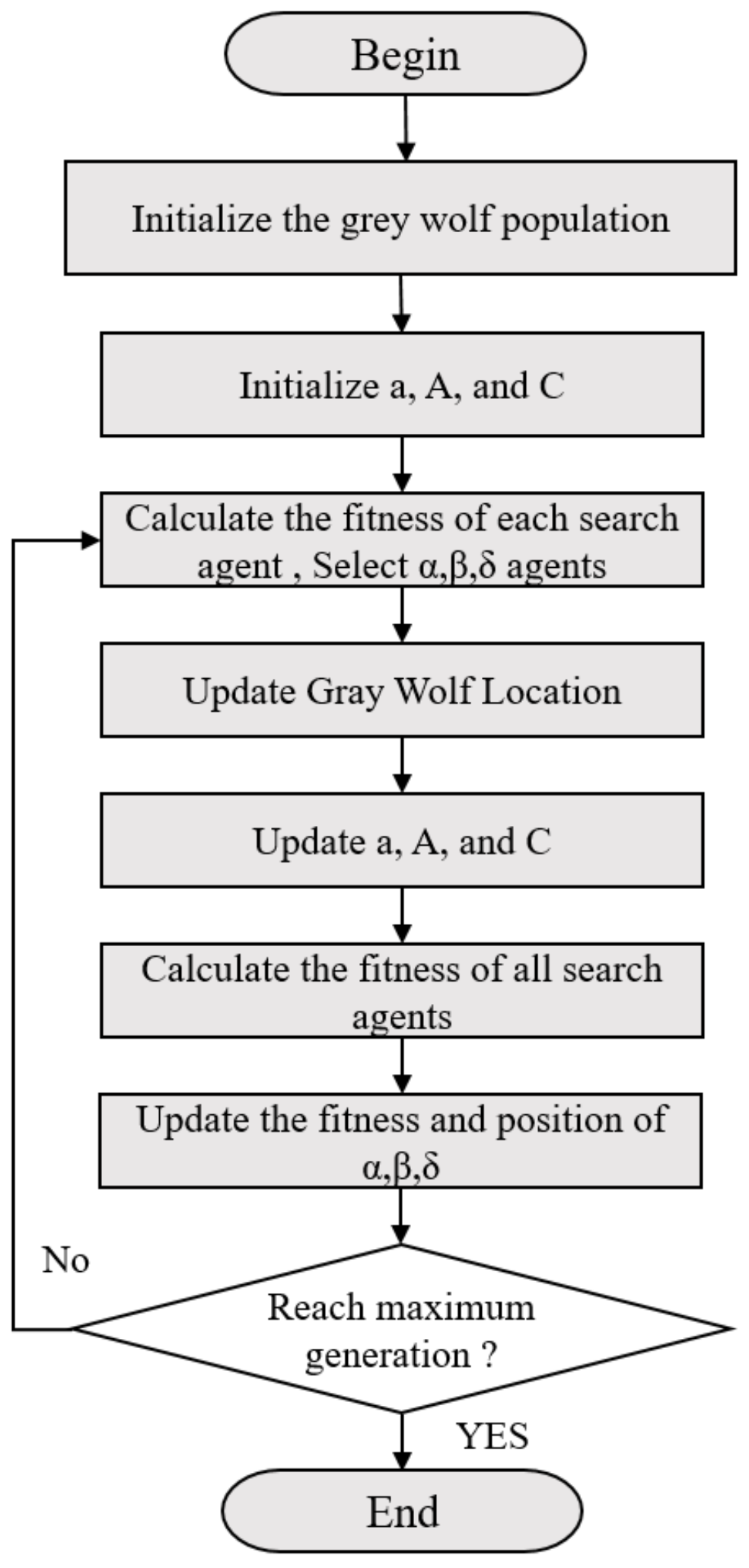
2.2. Grey Wolf Optimizer (GWO)

GWO, proposed by Mirjalili et al. [30], is a swarm intelligence algorithm inspired by wolves’ class system and prey predation process. In GWO, the fittest solution is named alpha ( α ), the second and third-best solutions are named beta ( β ) and delta ( δ ). The other candidate solutions are assumed to be omega ( ω ). In the GWO algorithm, the hunting (optimization) is guided by α , β and δ . The ω wolves follow the above three kinds of wolves.
Grey wolves will encircle their prey during hunting. The mathematical model of the enveloping behavior is shown as follows:
D = C · X P t X ( t  
X t + 1 = X P t A · D  
where t indicates the current iteration; A   and C are coefficient vectors; X P is the position vector of the prey;   X is the position vector of a grey wolf.
A and C are calculated as follows:
A = 2 a · r 1 a  
C = 2 · r 2  
where r 1 and r 2 are random vectors in [0, 1]; components of a are linearly decreased from 2 to 0 throughout iterations, and a is calculated as follows:
a = 2 2 t t m a x  
α usually guides the hunt. β and δ might also participate in hunting occasionally. The other search agents update their positions according to the best search agent. Such behavior can be formulated as follows:
D α = C 1 · X α X D β = C 2 · X β X D δ = C 3 · X δ X  
X 1 = X α A 1 · D α X 2 = X β A 2 · D β X 3 = X δ A 3 · D δ  
X t + 1 = X 1 + X 2 + X 3 3  
It is worth noting that when   A > 1 , the grey wolves will expand the encirclement and mainly conduct a global search. When A < 1 , the grey wolves narrow the encirclement to hunt the prey, mainly conducting a local search finally. Moreover, A with the number of iterations is influenced by Equations (5) and (7).
The pseudo code of GWO algorithm is shown in Algorithm 1. The computation process of basic GWO is shown in Figure 1.
Algorithm 1: Pseudo code of the GWO algorithm
Initialize the grey wolf population Xi (i = 1, 2, …, n)
Initialize a, A, C
For Xi (i = 1, 2, …, n) do
Calculate fitness
End for
Save the first three best wolves as Xα, Xβ and Xδ
While (t < Max number of iterations)
For each search agent
  Update the position of the current search agent by Equations (9)–(11)
End for
 Update a, A, and C
For Xi (i = 1, 2, …, n) do
Calculate fitness
End for
 Update a Xα, Xβ and Xδ
t = t + 1
End while
Return Xα

2.3. Case Study

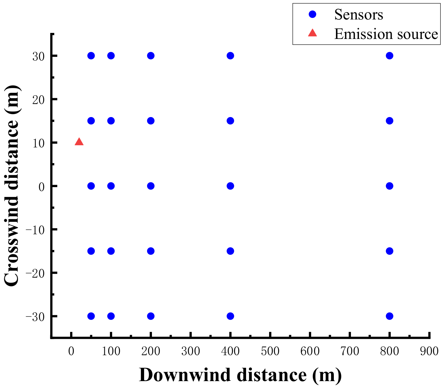
2.3.1. Simulation Cases

Simulation data from Gaussian plume models are used for comparing the performance of GWO with other optimization methods. Twenty-five sensors are set on the monitoring surface at the height of 1.5 m above ground, as shown in Figure 2. All sensors are assumed to be located downwind of the leak source, which is at point (30, 20) in the coordinate system. The wind speed is 2 m/s. The atmosphere is stable, rated “F” in the stability categories of Pasquill. The gas is emitted from a point source with a leakage rate of 8801.2 g/s. Seventeen of the Twenty-five sensors measured concentrations of more than 10−3, which were selected for emission source identification.

2.3.2. Experimental Cases

Simulation data from Gaussian plume models and experimental data from the Prairie grass experiment [31] are used for comparing the performance of GWO with other optimization methods. The parameters of the Gaussian plume model and each algorithm are the same as above. Run 17 and run 33 were selected from 68 sets of experimental results from the Prairie grass experiment.
In run 17, the leakage rate is 56.5 g/s, the height of the leakage source is 0.46 m, the wind speed is 2.87 m/s, the wind direction is 184°, the air temperature is 27.3 °C, and the atmospheric stability level is E, the leak source location was set to 94.6 and 66.8.
In run 33, The leakage rate is 94.7 g/s, the height of the leakage source is 0.46 m, the wind speed is 6.9 m/s, the wind direction is 181°, the air temperature is 29.1 °C, and the atmospheric stability level is ‘C’, the leak source location was set to 109 and 76.6.
The parameter settings of each algorithm are consistent with the reference [18,19,20,21,22,23,24,25,26]. For the PSO algorithm, the acceleration constant is set to 1.5. For the ACO algorithm, the pheromone volatility was set to 0.8, and the probability of route conversion was set to 0.2. For the GA method, the crossover probability is set to 0.6, and the variance probability is set to 0.7. The CPU is AMD Ryzen5 3600X with a calculation frequency of 3.8 GHz. The size of the population for all algorithms is 500, and the number of generations is 1000, and the results are averaged over 100 independent calculations. In the simulation case, the initial values of X, y and Q are [0, 1000], [−500, 500] and [0, 20,000], and in the experimental case, they are [0, 200], [−200, 200] and [0, 1000].

2.3.3. Skill Scores

A skill score is defined in reference [26] to assess the performance of different methods for evaluating source items. A smaller value of the skill score indicates a higher estimation accuracy. The skill scores of downwind positions, crosswind position and source strength are defined as relative errors, given as:
S i = r e s t , i r r e a l , i / r r e a l , i  
where i represents the corresponding source term (x, y, Q);   r e s t is the estimated value and r r e a l is the real value. The location score is calculated as follows:
S l = S x 2 + S y 2  
The average skill score of the source term is defined as:
S a = ( S l + S q ) / 2  

3. Results and Discussion

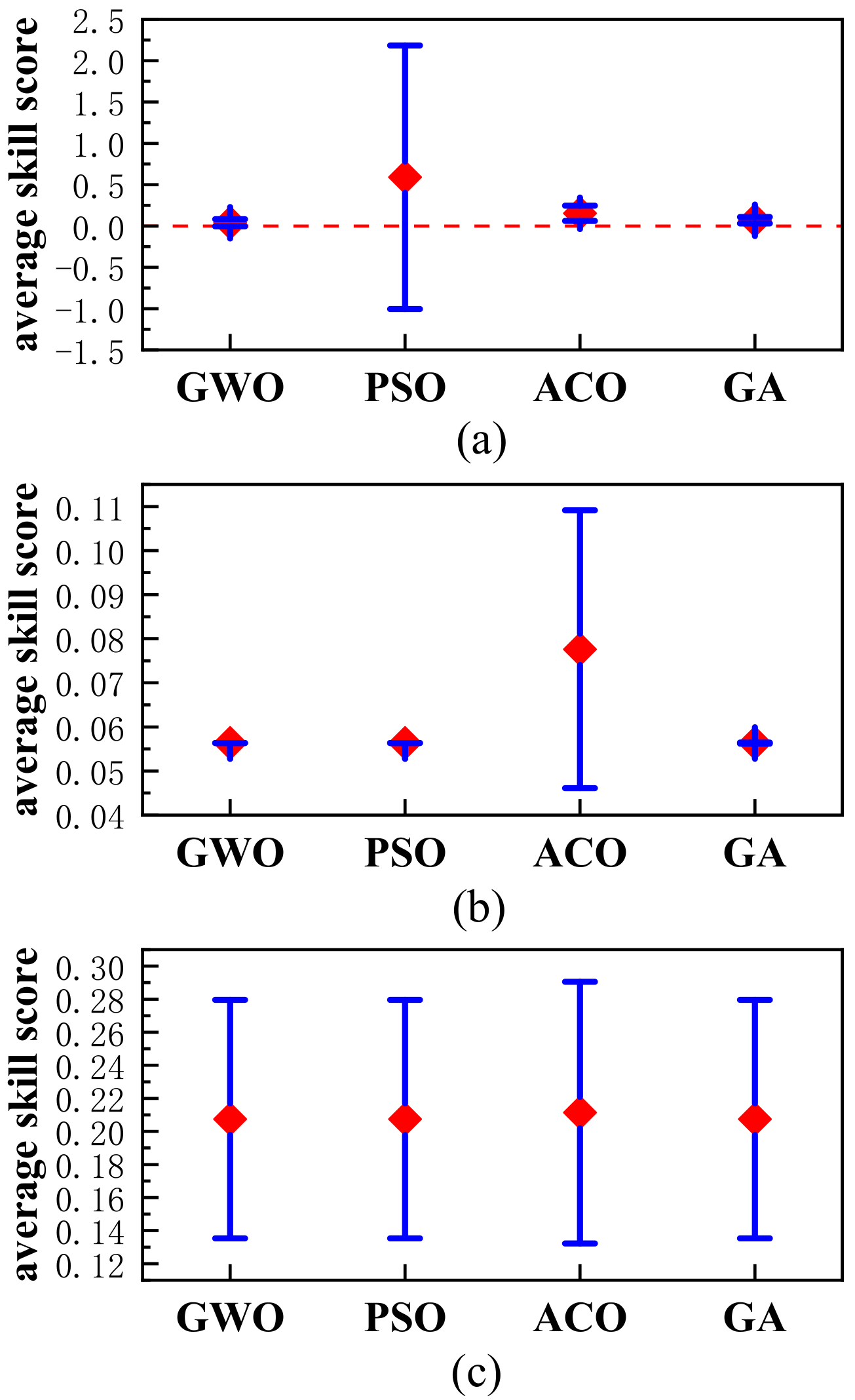
3.1. Estimation Results

The simulated data are used to compare the convergence performance of different algorithms in source term estimation, and the results are shown in Figure 3.
It can be seen that the final fitness values of GWO and PSO are close, and PSO converges faster. GWO performs self-adaptive convergence under the control of convergence factor. GWO converges faster in the early and late iterations, slower in the middle. As shown in Figure 3, PSO reaches convergence within 400 steps. GA reaches convergence within 500 steps, but the convergence accuracy is poor. The convergence of ACO is slow, and we can tell from Figure 3 that ACO does not reach convergence within 1000 steps. The convergence accuracy of GWO is the highest among the four methods.
Using the data from numerical simulation, run 17 and run 33 estimate the source parameters, and the results are shown in Table 1, Table 2 and Table 3. The average skill scores in the three STE cases are shown in Figure 4. The estimation of GWO takes a very short time, close to the GA with the shortest calculation time. GWO also performs extremely well in terms of estimation accuracy. PSO performs poorly in larger scenarios (simulation cases) due to the high initial value requirement of PSO. PSO is prone to premature convergence when the initial value is not appropriate, which seriously affects the estimation accuracy. ACO is very time-consuming and has low convergence accuracy at the population size and number of iterations described above. GA performs well in terms of estimation efficiency and accuracy. And GWO has the highest accuracy in several cases. The robustness of the STE for GWO is at the highest level in all cases. These algorithms perform differently in different scenarios. The GWO has advantages in each scenario. From the selected cases, some scenarios will indeed weaken the advantages of GWO algorithm, but will not eliminate these advantages. In summary, all four methods can successfully estimate the approximate information of emission sources. The GWO performs better among the four methods. The number of populations and iterations in this part of this paper are the same as in reference [25], which can be compared. The estimation efficiency and accuracy of GWO in this paper are better than the passive firefly algorithm (PFA) [25].
When estimating the source term by optimization algorithm, the number of populations, iterations and sensors are three factors playing essential roles in efficiency and accuracy. Therefore, the effects of these factors on estimation accuracy are discussed in the following section.

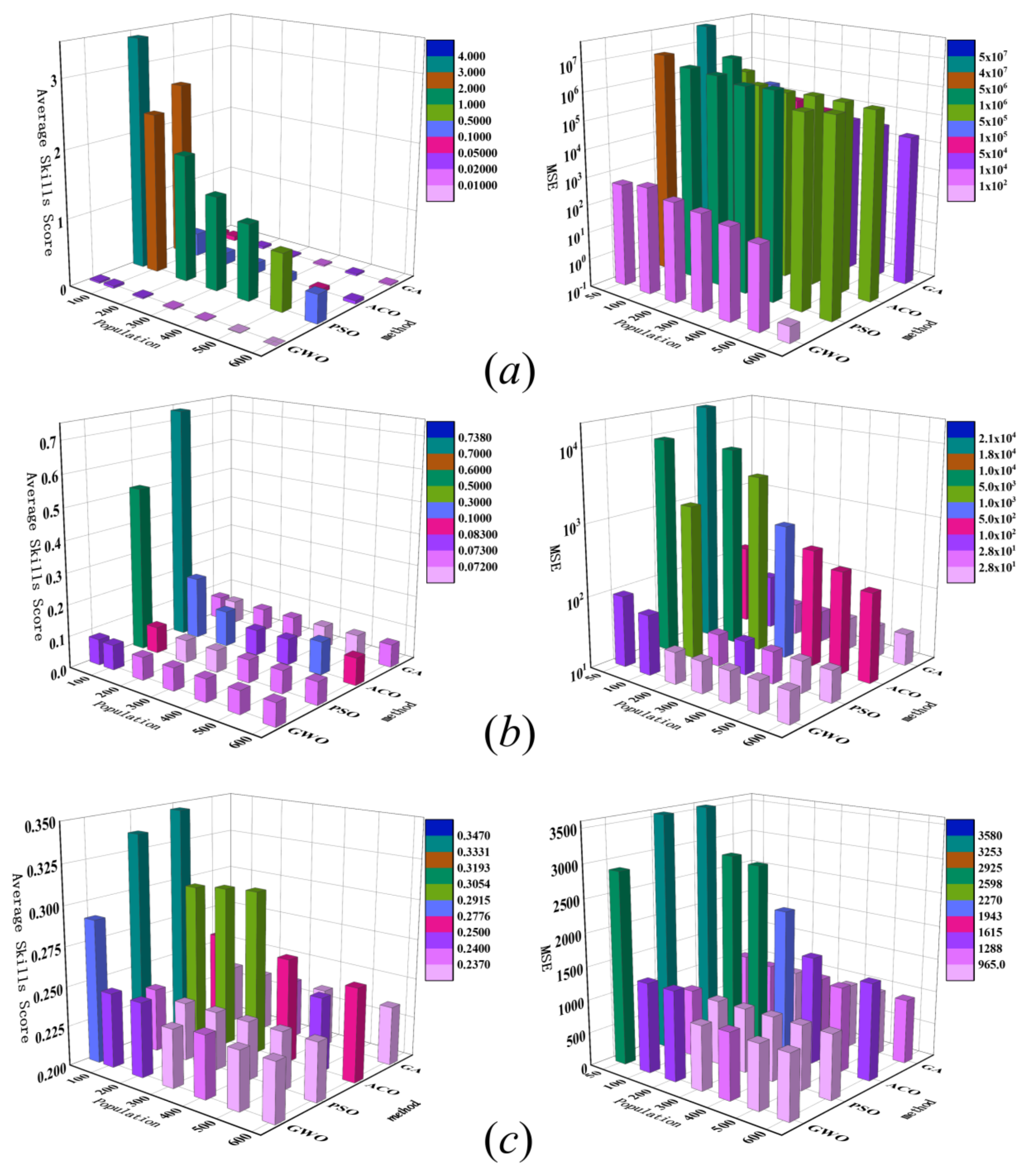
3.2. Effect of Population Size

Figure 5 shows the estimation results (the average skill score and MSE) of the five algorithms for the three cases under different population numbers (50–600), as the evidence for judgements of estimated accuracy and stability. All results are averaged by repeating the calculation 100 times.
The results demonstrate that the estimation accuracy and stability of the various methods improve with the increase in the population. In the experimental case, the estimation accuracy and stability of GWO, PSO and GA can reach almost the same level when the population size is large enough. In the simulation case, the advantage of high GWO convergence accuracy is revealed due to the absence of systematic errors. The performance of the GWO algorithm gets worse. As can be seen from the results of run 33, skill scores and MSE fluctuated with increasing population size and stabilized only when the population size reached 500. Therefore, in some cases, GWO requires a large population size to estimate emission source parameters more accurately. And in most cases (in the simulated case and run 33) GWO-based STE can effectively track the leak source at a smaller population size. Compared with reference [25], in run 17, the GWO population size reaches 200, and the accuracy reaches the highest number, while PFA requires a population size of 400. In run 33, the population size required for GWO to achieve the highest accuracy is also smaller than that of PFA.

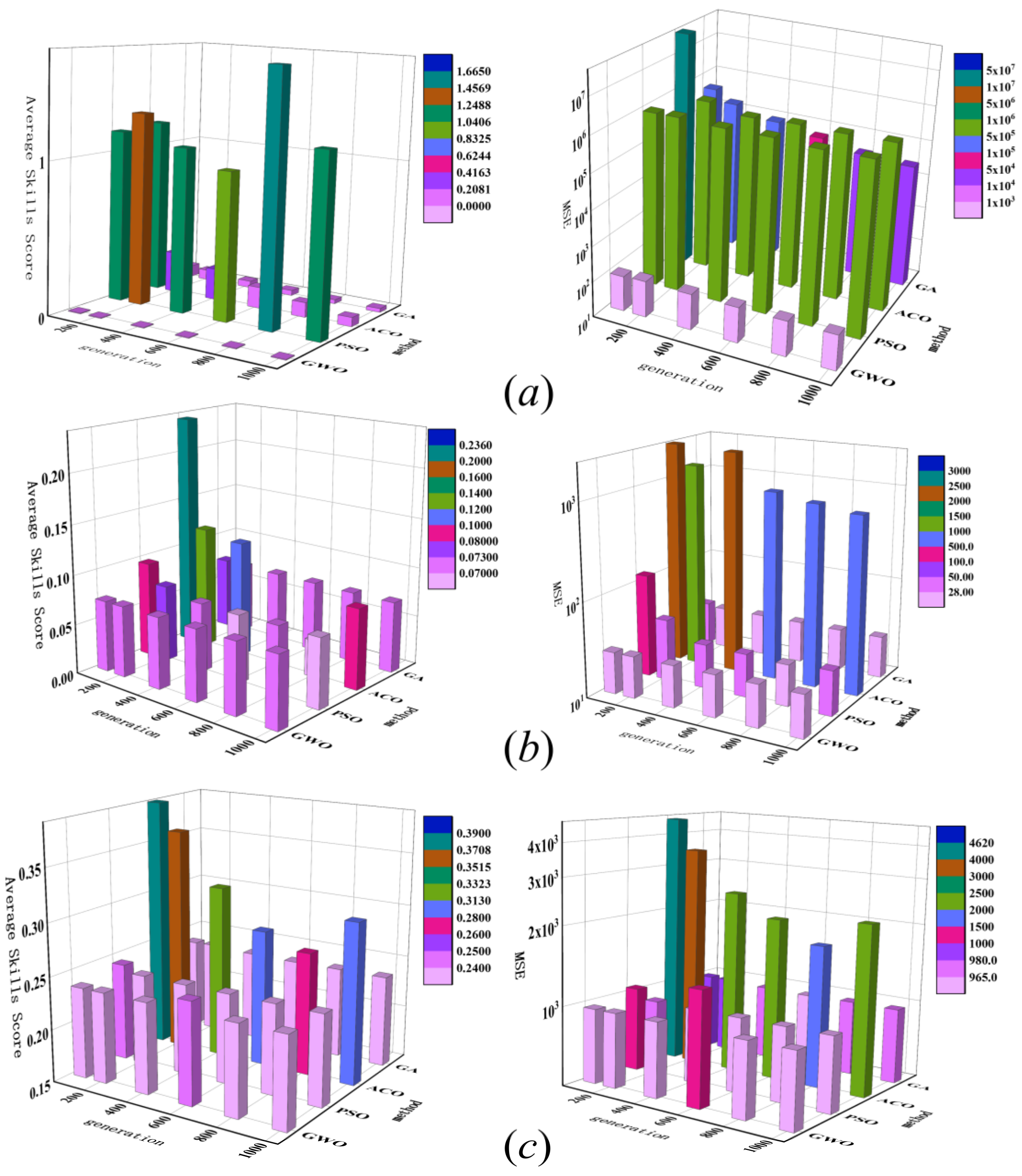
3.3. Effect of the Number of Iterations

The estimated source parameters obtained by GWO with different iterations numbers for three cases are compared with those of the other four algorithms in Figure 6.
The generation number is set in the range of 100–1000. It is noticeable that the estimation performance of ACO is more easily influenced by the number of iterations. The estimation accuracy and stability of PSO increase with the number of iterations when the number of iterations is small. Furthermore, GWO and GA are always stable in the number of iterations from 100 to 1000. And in the test of run 33, the accuracy of GWO suddenly deteriorates when the number of iterations is 600. This is due to the premature convergence of GWO. Also, this situation can show that the increase in iteration number does not reduce the chance of premature convergence. And the GWO-based STE at low number of iterations can have reliable estimation results.

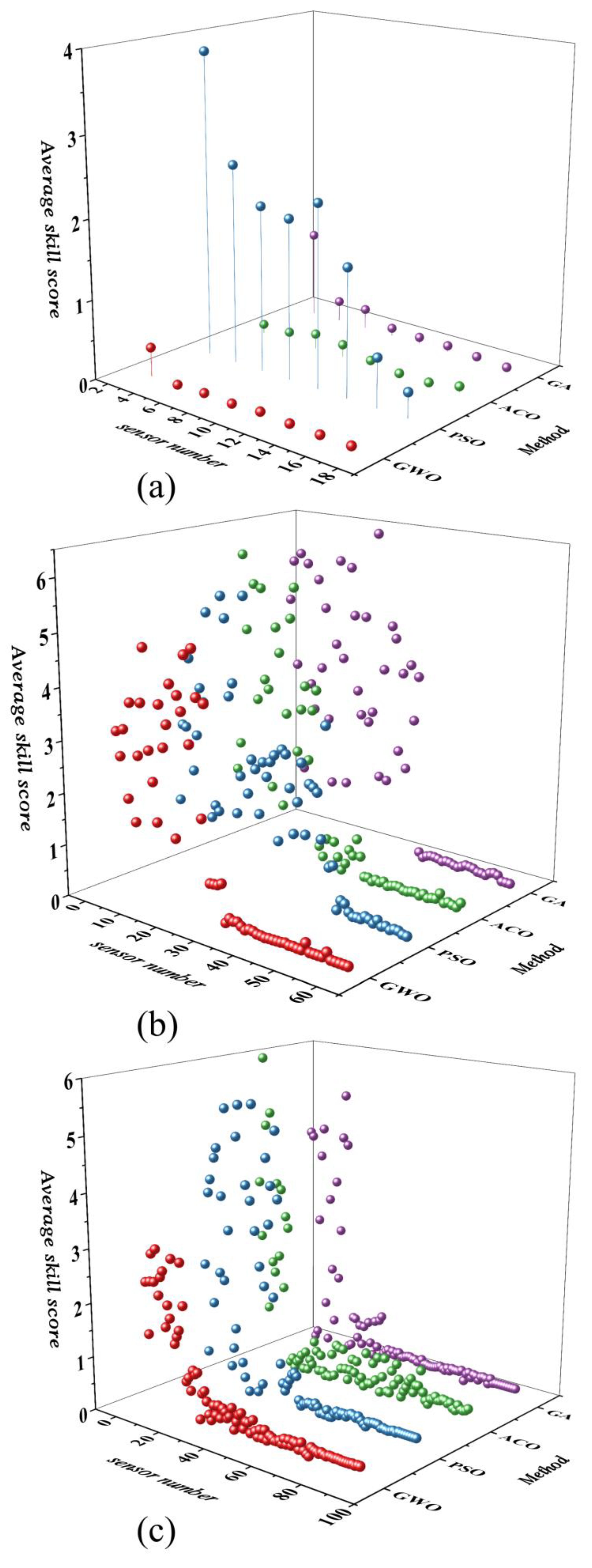
3.4. Effect of Sensor Number

The number of valid sensors affects the source term estimation. In the above three cases, the source terms were estimated using the concentrations of different numbers of effective sensors to investigate the effect on the estimation results. The skill scores estimated by four methods under different numbers of sensors are shown in Figure 7.
As shown in Figure 7, the average skill score of the various algorithms decreases with the increasing number of sensors. The number of sensors can have a significant impact on tracking emission sources. A threshold value for the number of sensors exists for each method. When the number of sensors reaches this threshold, the leak source parameters can be effectively estimated. As can be seen in Figure 7, the threshold is smaller for GWO than for other methods. Moreover, GWO is more robust than other methods when the number of sensors is less than the threshold. Therefore, GWO can obtain more accurate source term estimation results with fewer sensors than the other comparison methods. This is significant for the practical application of STE. A threshold value for the number of sensors exists for each method. However, GWO requires fewer sensors to achieve effective STE.

4. Gaussian Diffusion Model with Terrain Parameter Correction

The diffusion of gas leakage is a complex process, and any diffusion model has its own applicability and limitations. The Gaussian plume model makes idealized assumptions about complex turbulent processes and meteorological conditions for the sake of computational simplicity. These assumptions simplify the process of gas diffusion as well as the boundary conditions. Gaussian plume models are widely used in the study of forward diffusion and STE. However, the Gaussian plume model tends to produce large errors in practical application due to overly ideal assumptions. This can be reflected in the test of the experimental cases in this paper.
The diffusion of gases is influenced by the reflection of turbulence from the ground. The diffusion of gases can develop differently in various surface conditions, resulting in diverse diffusion results. Therefore, correction parameters controlled by topography are added to the Gaussian diffusion model. The range of values of the corresponding ground roughness z0 for different ground conditions is given in Table 4 [32].
The correction method of Gaussian plume model is as follows:
σ y = σ y 0 · f y  
σ z = σ z 0 · f z  
f y z 0 = 1 + a 0 z 0  
f z x , z 0 = b 0 c 0 l n x d 0 + e 0 l n x 1 z 0 f 0 g 0 l n x  
where σ y 0   and σ z 0 are the diffusion coefficient in the horizontal and vertical directions; f y and f z are the diffusion correction coefficients in the horizontal and vertical directions; and a 0 g 0 are a series of empirical correction factors, which have different values at different atmospheric stability.
Based on Table 5 and the experimental cases, a correction term with a roughness value of 0.1 is added to the Gaussian plume model in this section. Another control group with z0 = 0.2 and z0 = 0.3 are taken as the control group with unreasonable selection of roughness value. The performance of the modified Gaussian diffusion model in the GWO-based STE model is shown in Figure 8.
As shown in Figure 8, the highest estimation accuracy is achieved for z0 = 1. The estimation results for a suitable ground roughness (z0 = 0.1) are better than those without or with unreasonable corrections. The Gaussian plume model with correction has superior performance on STE. The method adopted in this section to correct the Gaussian plume model can effectively improve the accuracy of STE.

5. Conclusions

In this work, STE is investigated in terms of both optimization algorithm and diffusion model. A novel swarm intelligence algorithm, the GWO algorithm, has been used for estimating emission source parameters. Due to the adaptability feature, GWO has high convergence accuracy and estimated efficiency in STE. Compared with the other three algorithms, GWO has displayed satisfactory estimation accuracy and stability with acceptable estimation efficiency. As the number of populations and iterations increases, GWO is more robust than other methods. Although each of these methods requires a sufficient amount of sensor data to effectively estimate leak source information, GWO requires a smaller number of sensors than the other methods. Besides, GWO is more robust than other methods when the number of sensors is less than the threshold. After introducing corrections into the Gaussian plume model for different surface conditions, the results show improved calculation accuracy. It has proved that reasonable correction according to the ground roughness is an effective method for enhancing the accuracy of STE. All in all, the promising GWO algorithm is introduced to estimate the leakage source term, and the commonly used Gaussian plume model is modified to improve the accuracy of STE. Of course, GWO still suffers from premature convergence in tracking emission sources, which needs to be improved in subsequent studies. The following research can consider improving the convergence factor or adopting a hybrid strategy to improve the performance of GWO in STE.

Author Contributions

Conceptualization, methodology, software, data curation, writing—original draft preparation Y.L.; writing—review and editing, Y.J., X.Z. and Y.Q.; validation, resources, supervision Y.P. All authors have read and agreed to the published version of the manuscript.

Funding

This work was supported by Natural Science Fund for Distinguished Young Scholars of Jiangsu Province of China, grant number BK20190036.

Acknowledgments

This work was supported by Natural Science Fund for Distinguished Young Scholars of Jiangsu Province of China. Yong Pan acknowledged the sponsorship of Qing Lan Project.

Conflicts of Interest

The authors declare no conflict of interest. The funders had no role in the design of the study; in the collection, analyses, or interpretation of data; in the writing of the manuscript, or in the decision to publish the results.

Abbreviations

GWOGray Wolf optimizer
STEsource term estimation
PSOparticle swarm optimization
GAgenetic algorithm
ACOant colony optimization
SAsimulated annealing
BMCBayesian inference and stochastic Monte Carlo methods
MCMCMarkov chain Monte Carlo sampling method
BFGSBroyden-Fletcher-Goldfarb-Shanno algorithm
CFDComputational Fluid Dynamics
SCIPUFFThe Second-Order Closure Integrated Puff model
FAFirefly algorithm
PFAPassive firefly algorithm
AFAActive firefly algorithm

Nomenclatures

C o b s i Concentration measured by the sensor at the position i;
C p r e i Concentration predicted by the forward dispersion model;
NNumber of the measurement;
m i n f o b j Object function;
C(x, y, z)Gas concentration at position (x, y, z), g/m3;
uWind speed, m/s; Q is the emission source strength, g/s;
HHeight of the plume, m;
σ y   and   σ z Distance deviation coefficients in crosswind and vertical direction;
A   and C Coefficient vectors;
X P Position vector of the prey;
X Position vector of a grey wolf;
r 1 and r 2 Random vectors in [0, 1];
aConvergence factor;
tCurrent iteration number;
tmaxThe maximum number of iterations;
S i Skill score, where i represents the corresponding source term (x, y, Q);
S l Location score;
S a Average skill score;
r e s t The estimated value;
r r e a l The real value;
f y Diffusion correction coefficients in the horizontal direction;
f z Diffusion correction coefficients in the vertical direction;
a0–g0Empirical correction factors, which have different values at different atmospheric stability.

References

  1. Singh, S.K.; Rani, R. Assimilation of concentration measurements for retrieving multiple point releases in atmosphere: A least-squares approach to inverse modelling. Atmos. Environ. 2015, 119, 402–414. [Google Scholar] [CrossRef]
  2. Hutchinson, M.; Oh, H.; Chen, W.H. A review of source term estimation methods for atmospheric dispersion events using static or mobile sensors. Inf. Fusion 2017, 36, 130–148. [Google Scholar] [CrossRef] [Green Version]
  3. Sohn, M.D.; Reynolds, P.; Singh, N.; Gadgil, A.J. Rapidly locating and characterizing pollutant releases in buildings. Air Waste Manag. Assoc. 2002, 52, 1422–1432. [Google Scholar] [CrossRef] [PubMed]
  4. Sohn, M.D.; Sextro, R.G.; Gadgil, A.J.; Daisey, J.M. Responding to sudden pollutant releases in office buildings: 1. Framework and analysis tools. Indoor Air 2003, 13, 267–276. [Google Scholar] [CrossRef] [PubMed]
  5. Sohn, M.D.; Small, M.J.; Pantazidou, M. Reducing uncertainty in site characterization using Bayes Monte Carlo methods. Environ. Eng.-ASCE 2000, 126, 893–902. [Google Scholar] [CrossRef]
  6. Qian, S.S.; Stow, C.A.; Borsuk, M.E. On Monte Carlo methods for Bayesian inference. Ecol. Model. 2003, 159, 269–277. [Google Scholar] [CrossRef]
  7. Senocak, I.; Henuartner, N.W.; Short, M.B.; Daniel, W.B. Stochastic event reconstruction of atmospheric contaminant dispersion using Bayesian inference. Atmos. Environ. 2008, 42, 7718–7727. [Google Scholar] [CrossRef] [Green Version]
  8. Chow, F.K.; Kosovic, B.; Chan, S. Source inversion for contaminant plume dispersion in urban environments using building-resolving simulations. Appl. Meteorol. Climatol. 2008, 47, 1553–1572. [Google Scholar] [CrossRef] [Green Version]
  9. Yee, E.; Flesch, T.K. Inference of emission rates from multiple sources using Bayesian probability theory. Environ. Monit. 2010, 12, 622–634. [Google Scholar] [CrossRef]
  10. Xue, F.; Kikumoto, H.; Li, X.F.; Ooka, R. Bayesian source term estimation of atmospheric releases in urban areas using LES approach. Hazard. Mater. 2018, 349, 68–78. [Google Scholar] [CrossRef]
  11. Liu, Z.Z.; Li, X.F. The impact of sensor layout on Source Term Estimation in urban neighborhood. Build. Environ. 2022, 213, 108859. [Google Scholar] [CrossRef]
  12. Jia, H.Y.; Kikumoto, H. Sensor configuration optimization based on the entropy of adjoint concentration distribution for stochastic source term estimation in urban environment. Sust. Cities Soc. 2022, 79, 103726. [Google Scholar] [CrossRef]
  13. Ling, Y.S.; Huang, T.; Yue, Q.; Shan, Q.; Hei, D.; Zhang, X.; Shi, C.; Jia, W. Improving the estimation accuracy of multi-nuclide source term estimation method for severe nuclear accidents using temporal convolutional network optimized by Bayesian optimization and hyperband. J. Environ. Radioact. 2022, 424, 106787. [Google Scholar] [CrossRef] [PubMed]
  14. Eslinger, P.W.; Schrom, B.T. Utility of atmospheric transport runs done backwards in time for source term estimation. J. Environ. Radioact. 2019, 203, 98–106. [Google Scholar] [CrossRef]
  15. Singh, S.K.; Rani, R. A least-squares inversion technique for identification of a point release: Application to Fusion Field Trials 2007. Atmos. Environ. 2014, 92, 104–117. [Google Scholar] [CrossRef]
  16. Singh, S.K.; Sharan, M.; Issartel, J.P. Inverse modelling methods for identifying unknown releases in emergency scenarios: An overview. Int. J. Environ. Pollut. 2015, 57, 68–91. [Google Scholar] [CrossRef]
  17. Bieringer, P.E.; Rodriguez, L.M.; Vandenberghe, F.; Hurst, J.G.; Bieberbach, G., Jr.; Sykes, I.; Hannan, J.R.; Zaragoza, J.; Fry, R.N., Jr. Automated source term and wind parameter estimation for atmospheric transport and dispersion applications. Atmos. Environ. 2015, 122, 206–219. [Google Scholar] [CrossRef]
  18. Annunzio, A.J.; Young, G.S.; Haupt, S.E. A Multi-Entity Field Approximation to determine the source location of multiple atmospheric contaminant releases. Atmos. Environ. 2012, 62, 593–604. [Google Scholar] [CrossRef]
  19. Thomson, L.C.; Hirst, B.; Gibson, G.; Gillespie, S.; Jonathan, P.; Skeldon, K.D.; Padgett, M.J. An improved algorithm for locating a gas source using inverse methods. Atmos. Environ. 2007, 41, 1128–1134. [Google Scholar] [CrossRef]
  20. Pan, Y.; Jiang, J.C.; Wang, R.; Jiang, J.J. Predicting the net heat of combustion of organic compounds from molecular structures based on ant colony optimization. J. Loss Prev. Process Ind. 2011, 24, 85–89. [Google Scholar] [CrossRef]
  21. Qin, X.Q. A prediction model of mine gas emission base on a new ant colony algorithm. Appl. Mech. Mater. 2013, 318, 379–384. [Google Scholar] [CrossRef]
  22. Wang, Y.; Huang, H.; Huang, L.D.; Zhang, X.L. Source term estimation of hazardous material releases using hybrid genetic algorithm with composite cost functions. Eng. Appl. Artif. Intell. 2018, 75, 102–113. [Google Scholar] [CrossRef]
  23. Wang, Y.D.; Chen, B.; Zhu, Z.Q.; Wang, R.X.; Chen, F.R.; Yong, Z.; Zhang, L. A hybrid strategy on combining different optimization algorithms for hazardous gas source term estimation in field cases. Process Saf. Environ. Protect. 2020, 138, 27–38. [Google Scholar] [CrossRef]
  24. Ma, D.L.; Tan, W.; Zhang, Z.X.; Hu, J. Gas emission source term estimation with 1-step nonlinear partial swarm Optimization-Tikhonov regularization hybrid method. Chin. J. Chem. Eng. 2018, 26, 356–363. [Google Scholar] [CrossRef]
  25. Ma, D.L.; Gao, J.M.; Zhang, Z.X.; Wang, Q.S. An Improved Firefly Algorithm for Gas Emission Source Parameter Estimation in Atmosphere. IEEE Access 2019, 7, 111923–111930. [Google Scholar] [CrossRef]
  26. Ma, D.L.; Deng, J.Q.; Zhang, Z.X. Comparison and improvements of optimization methods for gas emission source identification. Atmos. Environ. 2013, 81, 188–198. [Google Scholar] [CrossRef]
  27. Wu, J.S.; Liu, Z.; Yuan, S.Q.; Cai, J.T.; Hu, X.F. Source term estimation of natural gas leakage in utility tunnel by combining CFD and Bayesian inference method. J. Loss Prev. Process Ind. 2020, 68, 104328. [Google Scholar] [CrossRef]
  28. Haupt, S.E.; Young, G.S.; Allen, C.T. Validation of a receptor-dispersion model coupled with a genetic algorithm using synthetic data. J. Appl. Meteorol. Climatol. 2007, 45, 476–490. [Google Scholar] [CrossRef]
  29. Briggs, G.A. Diffusion Estimation for Small Emissions; ATDL Contribution File No. 79; Atmospheric Turbulence and Diffusion Laboratory: Oak Ridge, TN, USA, 1973. [Google Scholar] [CrossRef] [Green Version]
  30. Mirjalili, S.; Mirjalili, S.M.; Lewis, A. Grey Wolf Optimizer. Adv. Eng. Softw. 2014, 69, 46–61. [Google Scholar] [CrossRef] [Green Version]
  31. Barad, M.L. Project Prairie Grass, a Field Program in Diffusion; Geophysical Research Paper, No. 59; Report AFCRC-TR-58-235(I); Air Force Cambridge Research Center: Cambridge, MA, USA, 1958; pp. 1–305. [Google Scholar]
  32. Zhang, W.; Zhang, X. Dispersion modeling of important toxic substance spills. J. Saf. Health Environ. 1996, 3, 1–19. [Google Scholar]
Figure 1. The flow chart of GWO algorithm. Where A is the convergence coefficient vector, C is the random coefficient vector, and a is the convergence factor.
Processes 10 01238 g001
Figure 2. Distribution of leakage source and sensors in simulation case.
Processes 10 01238 g002
Figure 3. The convergence process of different method.
Processes 10 01238 g003
Figure 4. The average skill scores in (a) simulation case, (b) run 17 and (c) run 33, represented by mean values (red diamond) and standard deviation (blue error bars).
Processes 10 01238 g004
Figure 5. Comparison results of different optimization algorithms with different population numbers in (a) simulation case, (b) run 17 and (c) run 33.
Processes 10 01238 g005
Figure 6. Comparison results of different optimization algorithms with different iterations numbers in (a) simulation case, (b) run 17 and (c) run 33.
Processes 10 01238 g006
Figure 7. Comparison results of different optimization algorithms with different numbers of valid sensors. (a) in simulation case, (b) in run 17 and (c) in run 33.
Processes 10 01238 g007
Figure 8. Performance of the modified Gaussian diffusion model in source term estimation.
Processes 10 01238 g008
Table 1. Source estimation results of different methods for simulation case.
MethodEstimation ResultsRelative ErrorMSEConsuming Time/s
x/my/mQ/g s−1xyQ
Real value30158801.20-----
GWO29.799914.99508799.170.67%0.03%0.02%399.463.11
PSO63.248915.08868584.18110.1%0.59%2.47%745,0104.12
ACO27.771015.00988703.317.43%0.06%1.11%536,57424.42
GA30.874715.06138734.842.92%0.41%0.75%37,644.63.01
Table 2. Source estimation results of different methods for run 17.
MethodEstimation ResultsRelative ErrorMSEConsuming Time/s
x/my/mQ/g s−1xyQ
Real value94.666.856.5-----
GWO92.548468.309661.09802.17%2.26%8.14%27.62941.51
PSO92.682368.308560.99591.20%2.26%7.87%28.51971.81
ACO90.790168.424663.02584.25%2.43%11.55%265.87314.79
GA92.531268.314861.10952.19%2.27%8.16%27.83341.46
Table 3. Source estimation results of different methods for run 33.
MethodEstimation ResultsRelative ErrorMSEConsuming Time/s
x/my/mQ/g s−1xyQ
Real value10976.694.7-----
GWO105.291081.9778126.7113.41%7.00%33.80%1348.42801.79
PSO105.804181.9892125.1062.93%7.02%32.11%963.76142.26
ACO103.5763581.8642131.7724.98%6.86%39.15%2077.85036.50
GA105.816781.9941125.0532.92%7.03%32.05%981.06361.73
Table 4. Range of ground roughness values for different surface conditions.
Surface Typesz0 (m)
Grassland or open country≤0.1
Crop areas0.1~0.3
Village or scattered trees0.3~1
urban1~4
Develop urban≥4
Table 5. The value of the coefficient a0g0.
Stability Class ABCDEF
a 0 g 0   Coefficient
a 0 0.0420.1150.150.380.30.57
b 0 1.101.51.492.532.42.913
c 0 0.03640.0450.01820.130.110.0944
d 0 0.43640.8530.870.550.860.753
e 0 0.050.01280.010460.0420.016820.0228
f 0 0.2730.1560.0890.350.270.29
g 0 0.0240.01360.00710.030.0220.023
Publisher’s Note: MDPI stays neutral with regard to jurisdictional claims in published maps and institutional affiliations.

