Practical Application-Oriented Energy Management for a Plug-In Hybrid Electric Bus Using a Dynamic SOC Design Zone Plan Method

Abstract

The main problem in current energy management is the ability of practical application. To address the problem, this paper proposes a reinforcement learning (RL)-based energy management by combining Tubule Q-learning and Pontryagin’s Minimum Principle (PMP) algorithms for a plug-in hybrid electric bus (PHEB). The main innovation distinguished from the existing energy management strategies is that a dynamic SOC design zone plan method is proposed. It is characterized by two aspects: ① a series of fixed locations are defined in the city bus route and a linear SOC reference trajectory is re-planned at fixed locations; ② a triangle zone will be re-planned based on the linear SOC reference trajectory. Additionally, a one-dimensional state space is also designed to ensure the real-time control. The off-line trainings demonstrate that the agent of the RL-based energy management can be well trained and has good generalization performance. The results of hardware in loop simulation (HIL) demonstrate that the trained energy management has good real-time performance, and its fuel consumption can be decreased by 12.92%, compared to a rule-based control strategy.

1. Introduction

The environmental pollution caused by the rapid development of the transportation industry cannot be ignored, and the electric vehicle is expected to solve this dilemma [1]. Plug-in hybrid electric vehicles (PHEVs), characterized by combining an electric motor and an internal combustion engine, can reduce gas emissions [2]. In practice, at least two power sources are deployed in the PHEV, that is, at least two degrees of freedom will be introduced into the energy management [3]. Therefore, energy management is the most important issue for the PHEVs [4,5].

Many energy management strategies such as rule-based, optimization–based, prediction-based, and reinforcement learning (RL)-based methods have been proposed. Nevertheless, no matter what methods are proposed, how to realize the real-time and economic control in real world is the objective of these methods. The rule-based energy management can easily realize real-time control in the real world. However, only when the key parameters are elaborately designed can the control performance improve. For example, Ding N. et al. proposed a hybrid energy management system based on a rule-based control strategy and genetic algorithm to improve the fuel economy and overcome the battery limitations [6]. Li P. et al. proposed an intelligent logic rule-based energy management method by optimizing the working area of the engine [7]. The optimization-based energy management can realize better economic control in the real world, although the real-time control performance may be sacrificed. For example, Hassanzadeh M. et al. proposed an energy management strategy based on PMP to improve the fuel economy and battery life in the uncertain traffic condition [8]. Wang W. et al. proposed an economic method based on dynamic programming (DP) and a feedback energy management system, which can maintain the state of charge of the battery (SOC) within the desired range [9]. Geng S. et al. compared various prediction methods and equivalent consumption minimization strategy (ECMS) implementations to evaluate the fuel consumption [10]. The prediction method-based energy management can realize real-time control in the real world, while the prediction precision should be well controlled. For example, Lian J. et al. proposed a predictive control algorithm by combining the long short-term memory network (LSTM) and the model predictive control (MPC) strategy to reduce fuel consumption under the constrains of SOC trajectory [11]. Liu Y J. et al. proposed a robust design method based on the Taguchi robust design method, where a nonlinear model predictive control (NMPC) is deployed to realize the real-time energy management [12]. In contrast, the RL-based energy management may be a promising method to realize real-time and economic control in the real world because it can realize self-learned control, thereby enhancing the control performance. For example, Lin X. et al. proposed an intelligent energy management strategy based on an improved RL algorithm with exploration factor to enhance the adaptability and improve the fuel economy [13]. Zhang H. et al. proposed a novel RL-based energy management method named Coach-Actor-Double Critic with a bi-level onboard controller to improve the self-leaning ability and adaptability [14]. However, the RL-based energy management also has some disadvantages that may hinder its practical application.

The RL-based energy management is mainly focused on the Q-learning (QL) algorithm. The easy implementation and good real-time control performances make the Tabular QL-based strategy the most popular method [15,16]. However, the problem of the “curse of dimensionality” is difficult to be avoided, once the state space is sufficiently large. Moreover, it can only solve the problem of discrete state and action. The key problem of RL-based energy management is to accurately identify the optimal action based on current state. As SOC should decline to the expected value at the destination, the best action may have a strong relationship with required power, velocity, and travelled distance for PHEV. Moreover, only when the state is adequately discrete can the action catch the best action [17]. Therefore, more than three states may be defined to ensure the strategy has good generalization performance. In this case, if every state is a discrete 100 segments, 1,000,000 states may be generated in the Q-table. This may lead to the “curse of dimensionality” problem, once the strategy is implemented into the currently used vehicle controller. Deep QL (DQL) based strategies can solve the continuous state space problem, which can avoid the “curse of dimensionality” problem by substituting the Q-table by a neural network model (NN) [18,19]. However, the control performance may deteriorate once the fitting precision of neural network (NN) is low. In contrast, Ref. [20] proposed an Action-Critic control framework (AC) to solve the problem of continuous state and action space. However, multiple NNs should be designed in the strategy. Therefore, it is difficult to implement into currently used controllers in order to realize real-time control, because the computation burden will be greatly increased. Similarly, Ref. [21] further proposed a deep deterministic policy gradient (DDPG) framework which considers the traffic information. However, it also has the similar problems as AC.

Thanks to the instantaneous optimization performance of Pontryagin’s Minimum Principle (PMP) and its easy implementable performance for the current vehicle controller, it is a feasible method to be used in real-world, once the co-state can be dynamically recognized [22,23]. So, if we combine the QL and the PMP as the recognition algorithm in a dynamical and uncertain traffic environment, the control performance may be enhanced. However, the “curse of dimensionality” problem should be avoided, if the real-time energy management control is to be satisfied. To solve this problem, Ref. [24] proposed a feasible method by designing the state as the difference between the feedback SOC and the reference SOC. Here, the SOC reference trajectory is designed by the optimal SOC trajectories calculated by a series of historical driving conditions. Inspired by this method, this paper proposes an RL-based energy management together with a similar state variable design method. In particular, the main difference between Ref. [24] and our work is that a dynamic linear SOC reference trajectory is planned at fixed locations based on the feedback SOC, and a triangle zone will be re-planned based on the reference SOC trajectory. The main advantage of this method is that the dynamic triangle zone can provide a margin for the fuel economy improvement, and can guide the feedback SOC reach the objective SOC.

The remainder of this paper is structured as follows. The modeling of the PHEB is introduced in Section 2. The RL-based energy management is detailed in Section 3. The results and discussion are presented in Section 4, and the conclusions are drawn in Section 5.

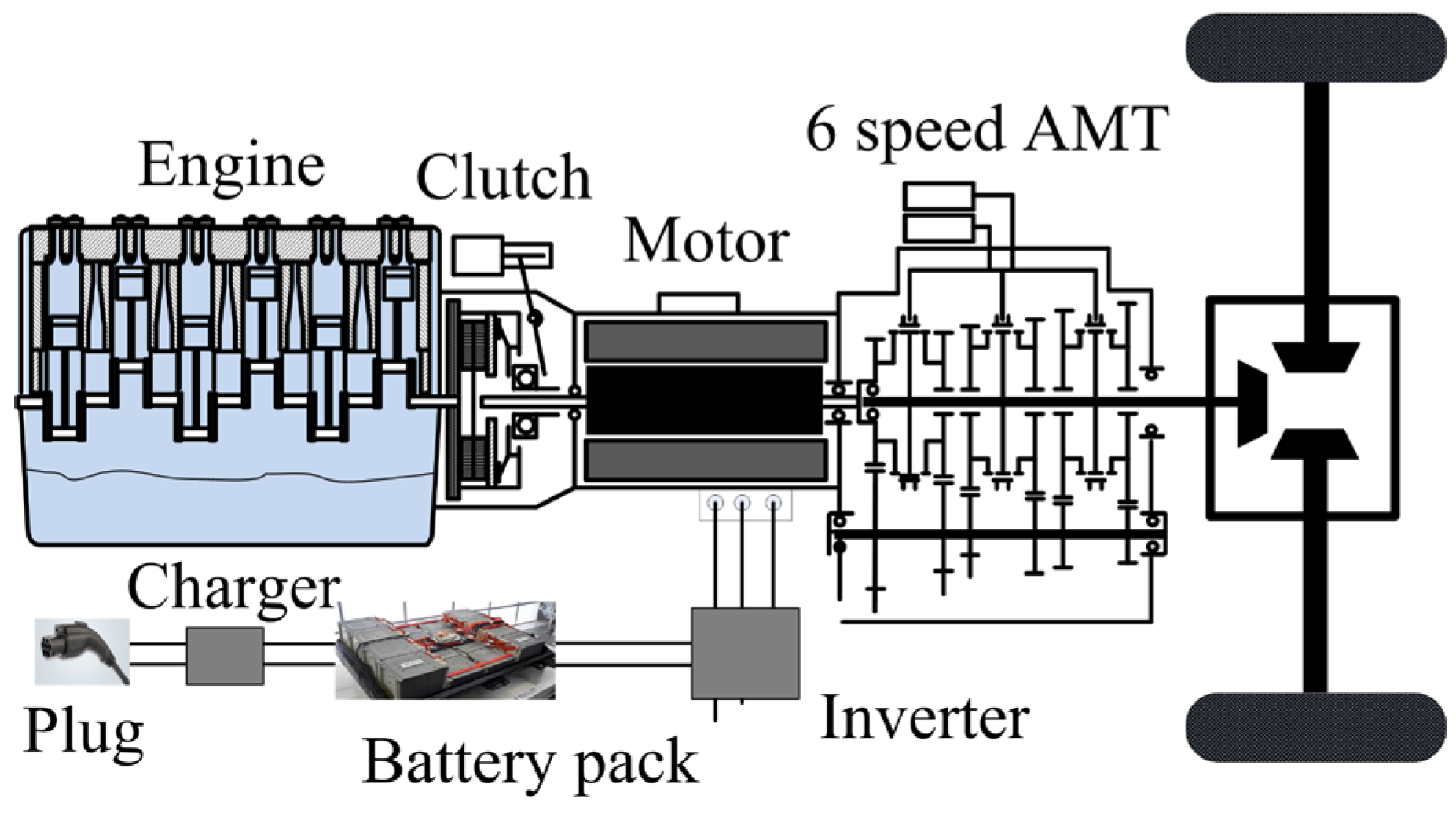
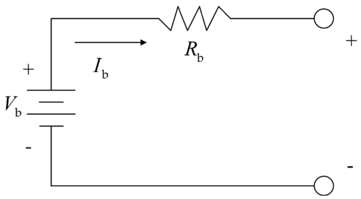
2. The Description of the PHEB

Figure 1 shows the layout of the PHEB. It is constituted by an engine, a clutch, an electric motor (EM), and a 6-speed automated mechanical transmission (AMT). The gears used in this paper are from 2 to 6, without considering the climbing driving conditions. Many working modes such as engine driving, hybrid driving, motor driving, and regenerative braking can be realized based on the driving demand and energy management.

An engine model that can satisfy the energy management requirement is indispensable. Based on the fuel consumption rate MAP of the engine (Figure 2), the instantaneous fuel consumption of the engine is formulated by

$$m_{\mathrm{e}}=\frac{T_{\mathrm{e}}\cdot n_{\mathrm{e}}}{9500}\cdot \frac{b_{\mathrm{e}}(T_{\mathrm{e}},n_{\mathrm{e}})}{3600}\cdot \Delta t$$

(1)

where $m_{\mathrm{e}}$ denotes the instantaneous fuel consumption of the engine; $T_{\mathrm{e}}$ denotes the torque of the engine; $n_{\mathrm{e}}$ denotes the speed of the engine; and $b_{\mathrm{e}}(T_{\mathrm{e}},{\omega }_{\mathrm{e}})$ denotes the fuel consumption rate of the engine.

Similarly, the motor is formulated by

$$\left\{\begin{array}{l}{P}_{\mathrm{m}}=n_{\mathrm{m}}\cdot T_{\mathrm{m}}\cdot {\eta }_{\mathrm{m}}{}^{-\mathrm{sgn}(T_{\mathrm{m}})}/9550\\ \mathrm{sgn}(T_{\mathrm{m}})=\left\{\begin{array}{l}1\hspace{1em}\hspace{1em}\hspace{1em}\mathrm{if}\hspace{1em}{T}_{\mathrm{m}}\ge 0\left(\mathrm{motoring} \mathrm{mode}\right)\\ -1\hspace{1em}\hspace{1em} \mathrm{if}\hspace{1em}{T}_{\mathrm{m}}<0\left(\mathrm{generating}\hspace{1em}\mathrm{mode}\right)\end{array}\right.\end{array}\right.$$

(2)

where $P_{\mathrm{m}}$ denotes the power of the motor; ${\eta }_{\mathrm{m}}$ denotes the efficiency of the motor, which can be interpolated by a look-up table formulated by the efficiency map of the motor (Figure 3); and $n_{\mathrm{m}}$ and $T_{\mathrm{m}}$ denote the speed and the torque of the motor, respectively.

As shown in Figure 4, the battery is formulated as a Rint model; it is described as

$$\left\{\begin{array}{l}S\dot{O}C=-\frac{1}{Q_{\mathrm{b}}}{I}_{\mathrm{b}}\\ I_{\mathrm{b}}=\frac{1}{2R_{\mathrm{b}}}(V_{\mathrm{b}}-\sqrt{V_{\mathrm{b}}{}^2-4R_{\mathrm{b}}{P}_{\mathrm{b}}})\end{array}\right.$$

(3)

where $V_{\mathrm{b}}$ denotes the battery voltage; $P_{\mathrm{b}}$ denotes the battery power; $R_{\mathrm{b}}$ denotes the internal resistance; and $Q_{\mathrm{b}}$ denotes the battery capacity.

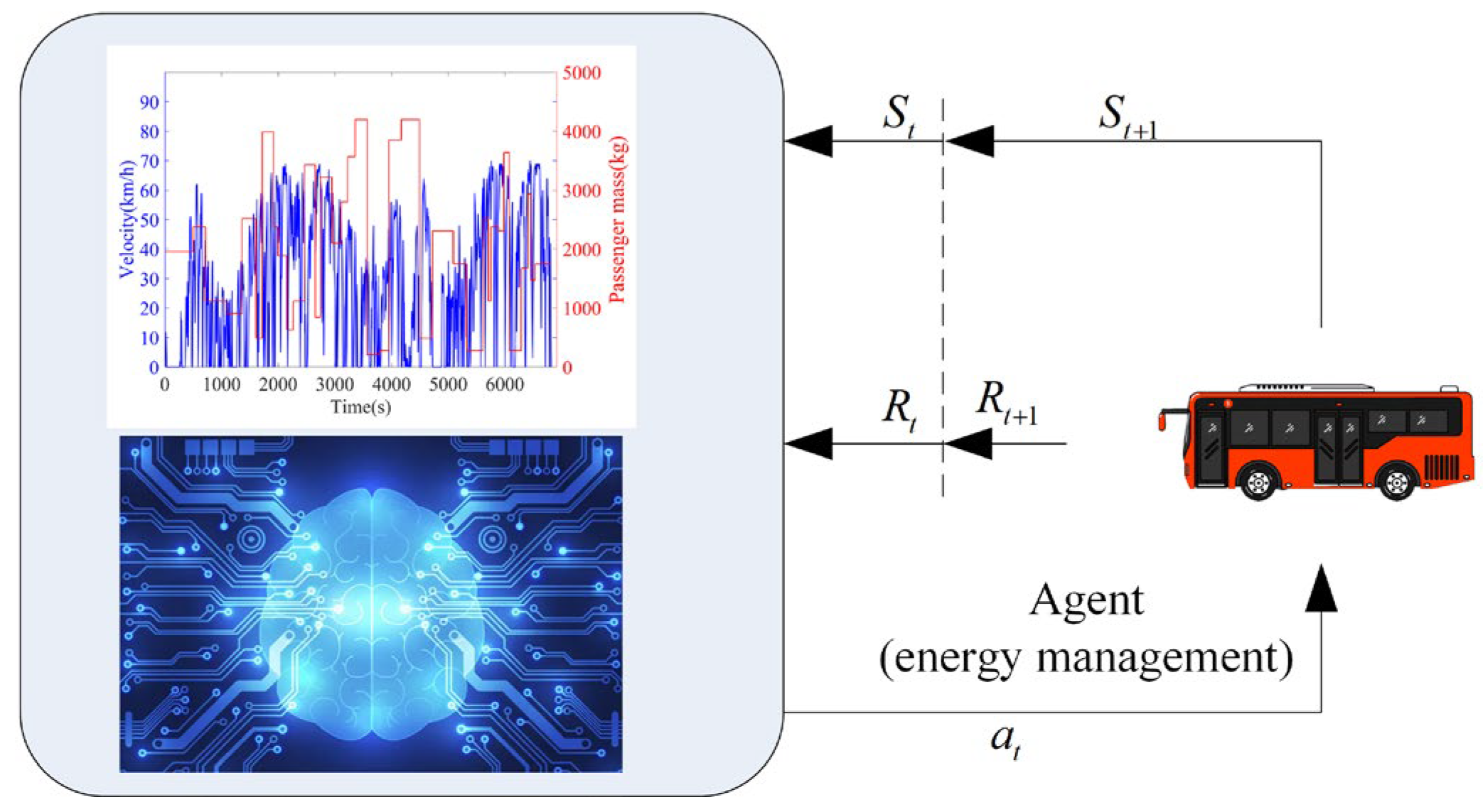
3. The Formulation of the RL-Based Energy Management

3.1. The Formulation of PMP

In this paper, an economic gear shift strategy is executed during shift process. In consideration of minimizing the fuel consumption, the objective function is described as

$$\min J={\displaystyle {\int }_{t_0}^{t_{\mathrm{f}}}\left[m_{\mathrm{e}}\left(u(t)\right)\right]\mathrm{d}t}$$

(4)

where $J$ denotes the performance index function and $u(t)$ denotes the control vector, which is the throttle of the engine ($u(t)=[th(t)]$). Here, the throttle of the engine is denoted by $th(t)$, which ranges from 0 to 1.

Inspired by Ref. [25], the energy management can be converted into instantaneous optimization problem by minimizing the Hamiltonian function, which can be described as

$$\left\{\begin{array}{l}H(x(t),u(t),\lambda (t),t)=m_{\mathrm{e}}(u(t))+\lambda (t)\cdot S\dot{O}C(t)\\ u^{*}(t)=\arg \min \left\{\left.H(x(t),u(t),\lambda (t),t)\right\}\right.\\ S\dot{O}C(t)=-\frac{V_{\mathrm{b}}(x(t))-\sqrt{V_{\mathrm{b}}^2(x(t))-4R_{\mathrm{b}}(x(t))P_{\mathrm{b}}(u(t))}}{2R_{\mathrm{b}}(x(t))Q_{\mathrm{b}}}\end{array}\right.$$

(5)

where $u^{*}(t)$ denotes the optimum control solution; $H(x(t),u(t),\lambda (t),t)$ denotes the Hamiltonian function, whereby the first term is the instant fuel consumption, and the second term is the delta SOC which is multiplied by co-state; and $\lambda (t)$ denotes the co-state.

Theoretically, the co-state is the only key parameter to influence the optimization performance and is a time-varied value. It can be also approximately recognized as constant over the whole trip, based on Refs. [22,23]. Moreover, it can also be adapted in real-time, based on the driving conditions [26].

Furthermore, some constraints, with respect to the physical components of the PHEB, are also indispensable, which is described as

$$\mathrm{S.t.} \left\{\begin{array}{l}{\omega }_{\mathrm{e\_min}}\le {\omega }_{\mathrm{e}}\left(t\right)\le {\omega }_{\mathrm{e\_max}}\\ {\omega }_{\mathrm{m\_min}}\le {\omega }_{\mathrm{m}}\left(t\right)\le {\omega }_{\mathrm{m\_max}}\\ P_{\mathrm{e\_min}}\left({\omega }_{\mathrm{e}}\left(t\right)\right)\le P_{\mathrm{e}}\left(t\right)\le P_{\mathrm{e\_max}}\left({\omega }_{\mathrm{e}}\left(t\right)\right)\\ P_{\mathrm{m\_min}}\left({\omega }_{\mathrm{m}}\left(t\right)\right)\le P_{\mathrm{m}}\left(t\right)\le P_{\mathrm{m\_max}}\left({\omega }_{\mathrm{m}}\left(t\right)\right)\end{array}\right.$$

(6)

where ${\omega }_{\mathrm{e}}(t)$ and ${\omega }_{\mathrm{m}}(t)$ denote the rotate speeds of the engine and the motor, respectively; ${\omega }_{\mathrm{e\_min}}$, ${\omega }_{\mathrm{e\_max}}$ and ${\omega }_{\mathrm{m\_min}}$, ${\omega }_{\mathrm{m\_max}}$ denote the corresponding rotate speed boundaries; $P_{\mathrm{e}}(t)$ and $P_{\mathrm{m}}(t)$ denote the powers of the engine and the motor, respectively; and $P_{\mathrm{e\_min}}$, $P_{\mathrm{e\_max}}$ and $P_{\mathrm{m\_min}}$, $P_{\mathrm{m\_max}}$ denote the corresponding power boundaries.

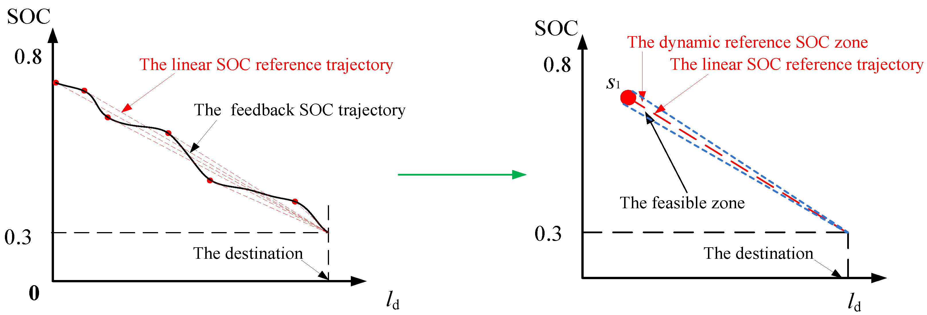
3.2. The Design of the Dynamic SOC Design Zone

In this paper, only one state for the difference between the feedback SOC and reference SOC trajectory is designed for the RL-based energy management. Therefore, the SOC reference trajectory becomes the key issue. As shown in Figure 5, a novel dynamic SOC design zone plan method is proposed. The basic principle is that a linear SOC reference trajectory will be firstly planned at the fixed location, and simultaneously a dynamic reference SOC zone will be defined based on the linear SOC reference trajectory. There are two advantages to this method.

(1). The state of the difference of SOC between the dynamic reference SOC and the feedback SOC is only defined. In this case, only a Q-matrix with 100 rows and 27 columns is designed, which can ensure the real-time control of the strategy.

(2). In practice, the real driving conditions cannot be completely predicted, so the optimal SOC trajectory is usually not completely predicted. In this case, taking the optimal SOC trajectory as reference trajectory is infeasible. However, if a feasible zone (the floating value is designed as 0.02) is defined based on the liner SOC reference trajectory, the feedback SOC may be controlled within a feasible zone, and a great margin for the fuel economy improvement may be provided. This is also the most important innovation in this paper.

The main difference between the proposed method and the existing methods are listed as follows.

(1). In Ref. [24], only a SOC reference trajectory is designed, based on a series of optimal SOC trajectories. In terms of our method, the SOC reference trajectory is only based on the fixed location. Moreover, a triangle zone will be also defined to improve the fuel economy of the PHEB.

(2). In Ref. [25], only an efficient zone is defined based on a series of optimization SOC trajectories, and no dynamic reference SOC trajectory is planned. Moreover, three states should be designed, and the efficient zone is designed off-line.

In addition, the dynamic SOC design zone plan method can be described as

$$\left\{\begin{array}{l}SO{C}_{\mathrm{ref}}=\frac{SO{C}_{\mathrm{T}}-SO{C}_{\mathrm{fnl}}}{D_{\mathrm{T}}-D_{\mathrm{fnl}}}\cdot \left(D_{\mathrm{ref}}-D_{\mathrm{fnl}}\right)+SO{C}_{\mathrm{fnl}}\\ SO{C}_{\mathrm{upper}}=\frac{SO{C}_{\mathrm{T}}+0.02-SO{C}_{\mathrm{fnl}}}{D_{\mathrm{T}}-D_{\mathrm{fnl}}}\cdot \left(D_{\mathrm{ref}}-D_{\mathrm{fnl}}\right)+SO{C}_{\mathrm{fnl}}\\ SO{C}_{\mathrm{lower}}=\frac{SO{C}_{\mathrm{T}}-0.02-SO{C}_{\mathrm{fnl}}}{D_{\mathrm{T}}-D_{\mathrm{fnl}}}\cdot \left(D_{\mathrm{ref}}-D_{\mathrm{fnl}}\right)+SO{C}_{\mathrm{fnl}}\end{array}\right.$$

(7)

where $SO{C}_{\mathrm{ref}}$ and $D_{\mathrm{ref}}$ denote the reference SOC and travelled distance at current time step, respectively; $SO{C}_{\mathrm{T}}$ and $D_{\mathrm{T}}$ denote the dynamic value of target SOC and the travelled distance, respectively, which are updated after fixed distance step; and $SO{C}_{\mathrm{fnl}}$ and $D_{\mathrm{fnl}}$ denote the value of target SOC and travelled distance at destination, respectively.

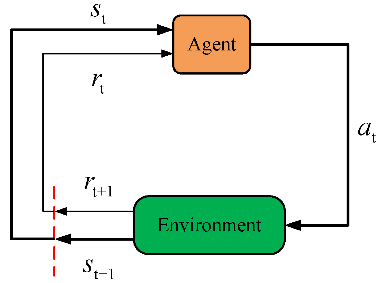
3.3. The Formalation of the RL-Based Energy Managemtn

QL is one of the most important RL methods, based on the Temporal-Difference (TD) method. The update process of the Q value can be described as

$$Q(s_t,a_t)\leftarrow Q(s_t,a_t)+\alpha \left[r_{t+1}+\gamma \underset{a}{\max }Q(s_{t+1},a)-Q(s_t,a_t)\right]$$

(8)

where $\alpha$ denotes the learning rate, which is defined as 0.95 in this paper; $\gamma$ denotes the discount factor, which is defined as 0.8 in this paper; $r_{t+1}$ denotes the immediate reward at time $t$; and $\underset{a}{\max }Q(s,a)$ denotes the maximum Q value in the next state.

As shown in Figure 6, at every time step, the agent will obtain a state $S_t$ from the environment, and an action $a_t$ will be evaluated by the agent. Then, a state of the environment $s_{t+1}$ will be adapted, and a corresponding reward $r_{t+1}$ will be transmitted to the agent.

As an instantaneous optimization algorithm, PMP-based energy management has good real-time control performance. The only challenge is to recognize the co-state for the unrepeatable, stochastic driving conditions. In addition, QL is widely regarded as an intelligent algorithm that can adapt well to uncertain circumstances. Motivated by this, an RL-based energy management, combining PMP and RL, is proposed. As shown in Figure 7, at every time step, the agent will evaluate an action based on the states, and the states of PHEB will be adapted based on the action, then a reward will be generated and transmitted to the agent.

(1)

The state

As stated above, the difference between the feedback SOC and the reference SOC is defined as the sole state, which is descried as

$$s_t=SO{C}_{\mathrm{f}}-SO{C}_{\mathrm{ref}}$$

(9)

where $SO{C}_{\mathrm{f}}$ denotes the feedback SOC. The state $s_t$ ranges from −0.04 to 0.04, and is sampled by 100 points. That is to say, the number of rows is only 100, which provides a basis to reduce the dimensionality of the Q and R tables.

(2)

The action

The co-state is defined as the only action, which ranges from −2800 to −4000. Specifically, the action space is

$$a_t=\left[\begin{array}{l}-2800,-2900,-3000,-3100,-3200,-3250,-3275,-3300,-3325,-3350,-3375,-3390,-3400,\\ -3410,-3425,-3450,-3475,-3500,-3525,-3550,-3575,-3600,-3650,-3700,-3800,-3900,-4000\end{array}\right]$$

(10)

(3)

The reward

As stated above, the reward is defined as Equation (11). Specifically, if the feedback SOC at time step $t+1$ is larger than the upper boundary, then a punishment will be provided to the Q-value function. Moreover, the further the deviation is, the greater the punishment will be; if the feedback SOC at time step $t+1$ is lower than the lower boundary, then a punishment will be provided to the Q-value function. Moreover, if the feedback SOC at time step $t+1$ located in the feasible zone (between the lower and upper boundaries), a reward will be provided to the Q-value function, and the closer the feedback SOC to the reference, the greater the reward will be.

$$r_t=\left\{\begin{array}{l}-abs(SO{C}_{\mathrm{f}}(t+1)-SO{C}_{\mathrm{upper}}(t+1))\hspace{1em}\hspace{1em}\hspace{1em}\hspace{1em}SO{C}_{\mathrm{f}}(t+1)>SO{C}_{\mathrm{upper}}(t+1)\\ -abs(SO{C}_{\mathrm{f}}(t+1)-SO{C}_{\mathrm{lower}}(t+1))\hspace{1em}\hspace{1em}\hspace{1em}\hspace{1em}SO{C}_{\mathrm{f}}(t+1)<SO{C}_{\mathrm{lower}}(t+1)\\ \frac{10}{1+100\ast \mathrm{abs}(SO{C}_{\mathrm{f}}(t+1)-SO{C}_{\mathrm{r}}(t+1))}\hspace{1em}\hspace{1em}\hspace{1em}\hspace{1em}\hspace{1em}\hspace{1em}\hspace{1em}\hspace{1em}SO{C}_{\mathrm{lower}}(t+1)\le SO{C}_{\mathrm{f}}(t+1)\le SO{C}_{\mathrm{upper}}(t+1)\end{array}\right.$$

(11)

(4)

The ε-greedy algorithm

To realize the self-learning control, the ε-greedy algorithm is deployed, which is formulated by

$${\pi }^{\ast }(a|s)=\left\{\begin{array}{l}a=\mathrm{random}(A)\hspace{1em}\mathrm{if} r_{\mathrm{n}}<\epsilon \\ a=\underset{}{\max }Q(s,a)\hspace{1em}\mathrm{if} r_{\mathrm{n}}\ge \epsilon \end{array}\right.$$

(12)

where $r_{\mathrm{n}}$ is the random number, which ranges from 0 to 1.

(5)

The RL-based energy management algorithm

1: initializing the Q and R tables with null matrix

2: for episode = 1, M do

3:  for t = 1, T do

4:    observing the current state $s_t$ ($s_t=SO{C}_{\mathrm{f}}-SO{C}_{\mathrm{ref}}$)

5:    selecting the action $a_t$ with ε-greedy algorithm

6:    executing the action($a_t$) and observing the next state

7:    calculating the immediate reward based on Eq. (11)

8:    updating the Q-Table by: $Q(s_t,a_t)\leftarrow Q(s_t,a_t)+\alpha \left[r_{t+1}+\gamma \underset{a}{\max }Q(s_{t+1},a)-Q(s_t,a_t)\right]$

9:  end

10:  if the feedback SOC is bigger than 0.85 or lower than 0.25 or abs ($s(t)$) is bigger than 0.04 11:   continue;

12:  end

13:  end

14: end

As shown in Figure 8, the design process is divided into three steps: off-line training, off-line verification, and hardware in the loop (HIL) with controller.

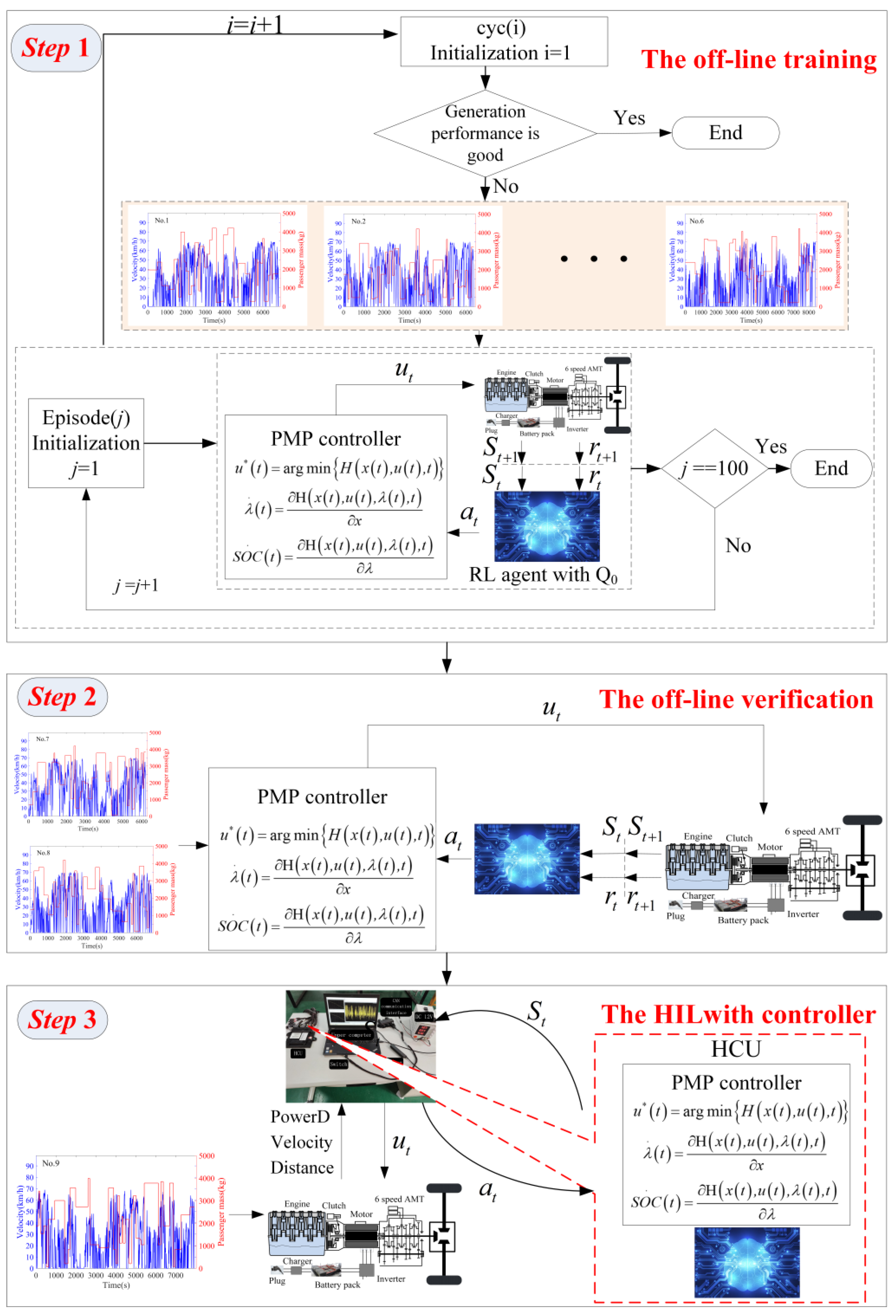
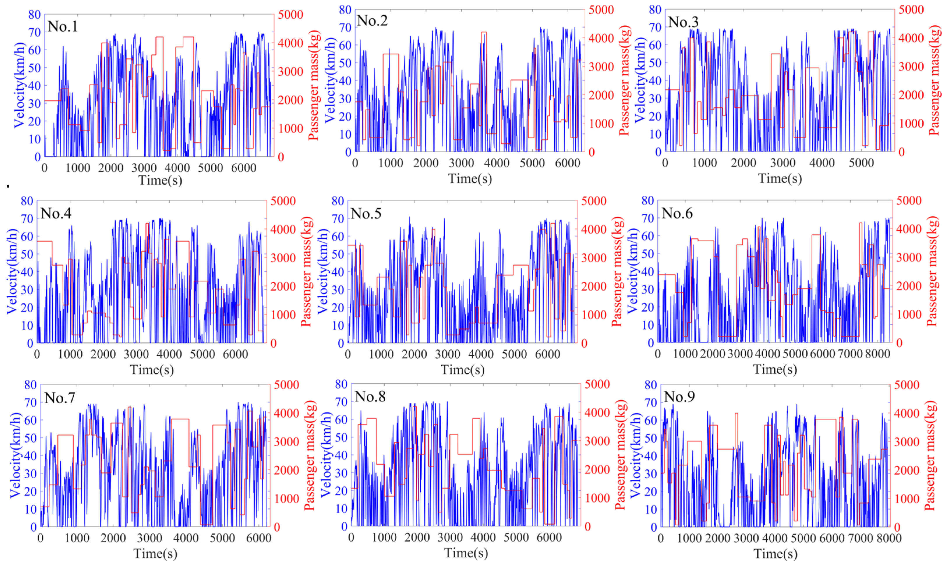
4. Result Discussions

A series of historical driving cycles of the PHEB are deployed for training and testing. The total length of route is about 50 km and has 39 bus stops; the number of passengers at per station is assumed to be random. Moreover, as shown in Figure 9, a series of combined driving cycles, including driving cycle and passenger mass, are designed in this paper.

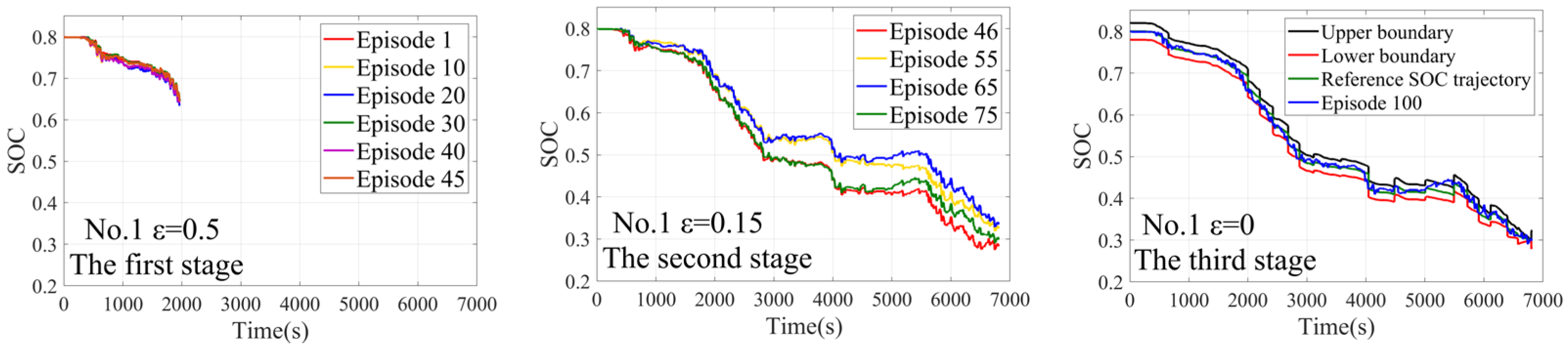
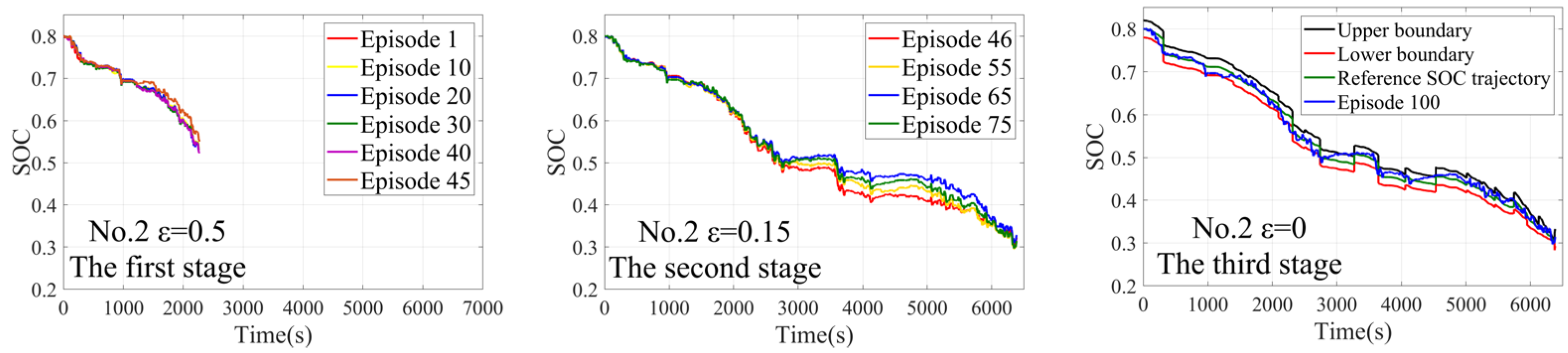
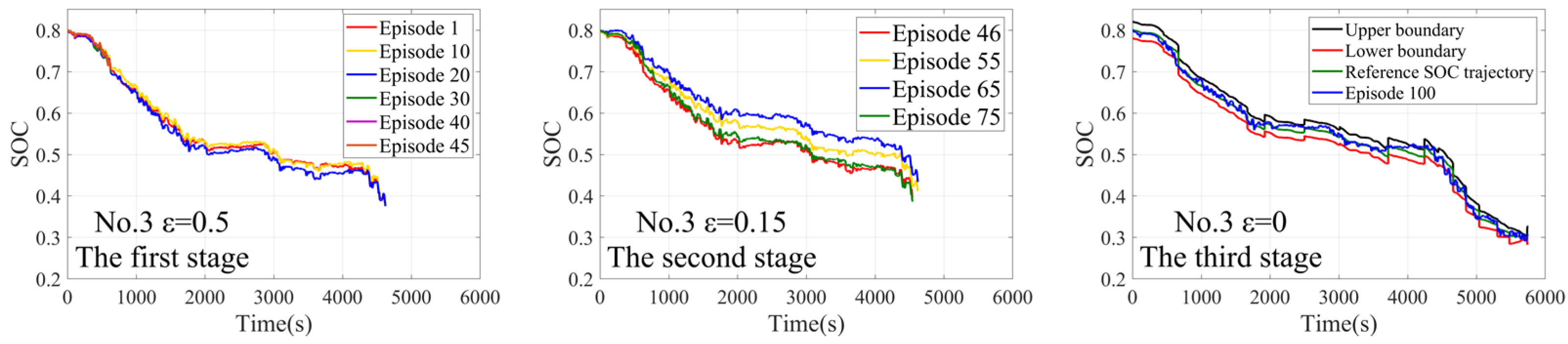
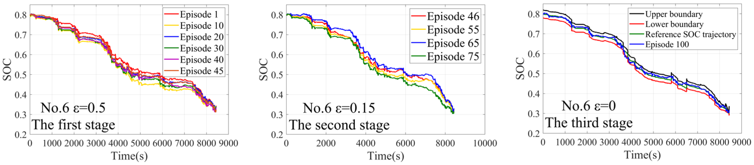
4.1. The Training Process

To ensure the RL-based energy management has better control performance, a well-trained Q-table of the reinforcement learning is indispensable. Therefore, six combined driving cycles are firstly designed to train the Q-table. The Q-table is continually trained one by one based on the combined driving cycles, and will be trained 100 times for each combined driving cycle based on different $\epsilon$ value. Specifically, the training is divided into three stages; in the first stage, the $\epsilon$ is designed as 0.5 before episode 45, which implies that the action is randomly selected by the probability of 50%; in the second stage, the $\epsilon$ is designed as 0.15 between the episode 46 and episode 75, which implies that the action is randomly selected by the probability of 15%; in the third stage, the $\epsilon$ is designed as 0 between the episode 76 and episode 100, which implies that the action is selected by the trained Q-table.

As shown in Figure 10, the combined driving cycle 1 is firstly selected to train the Q-table (named Q-table 1). In the first stage, the agent strives to probe the possible action. In this case, the final SOCs are higher than 0.6, which implies that the Q-table 1 is not well trained; in the second stage, the RL will partly select the action based on the trained Q-table 1, whilst trying to probe possible actions by the ε-greedy algorithm. In this case, the SOCs will be fluctuated around 0.3, which implies the Q-table 1 has been better trained. In the third stage, the final SOC can easily reach the objective vale, and the feedback SOC trajectory can easily follow the reference SOC trajectory. This implies that the Q-table 1 has been well trained for the combined driving cycle 1.

As shown in Figure 11, the combined driving cycle 2 is deployed to continually train the Q-table (Q-table 2), based on Q-table 1. The RL will still be terminated in advance in the first stage. Moreover, the final SOCs are higher than 0.5, which are lower than the final SOCs in Figure 10. In the second stage, the final SOCs can satisfy the control object, and has good control perforce. In the third stage, the Q-table has been well trained, the final SOC can satisfy the control object, and the SOC trajectory can better follow the reference SOC trajectory well. This implies that the Q-table 2 has been better trained compared to the Q-table in Figure 10.

As shown in Figure 12, the combined driving cycle 3 is deployed to continually train the Q-table (Q-table 3), based on the well trained Q-table 2. In the first stage, the control performance has been greatly improved, compared to the first stage for Q-table 1 and 2. However, the final SOCs still do not satisfy the control object. In contrast, the control preference is deteriorated in stage 2 compared to the Q-table 2. This implies that the driving conditions may be different from the combined driving cycle 2, and the generalization performance of the Q-table should be further improved. Nevertheless, the control preference can satisfy the control objective during the third stage, and it is recognized that the Q-table 3 has been well trained.

As shown in Figure 13, the combined driving cycle 4 is deployed to continually train the Q-table (Q-table 4), based on the well trained Q-table 3. Similar to the first stage in Figure 12, the Q-table 4 is also not well trained, because the final SOCs do not reach 0.3. However, the control performance is greatly improved in the second stage, and the control performance can satisfy the control objective in the stage 3. This implies that Q-table 4 has been well trained.

It can be seen from Figure 14 and Figure 15 that the Q-table 4 has been well trained, because the control performance can be well satisfied in three stages, no matter the $\epsilon$ value. This implies that the generalization performance of the Q-table 4 has been greatly improved, and can satisfy the control performance. On the other hand, the generalization performance of the Q-table 4 will be further improved based on the trainings of the two combined driving cycles. In addition, Q-table 6 can be taken as the well trained Q-table being after continually trained by combined driving cycle 5 and 6.

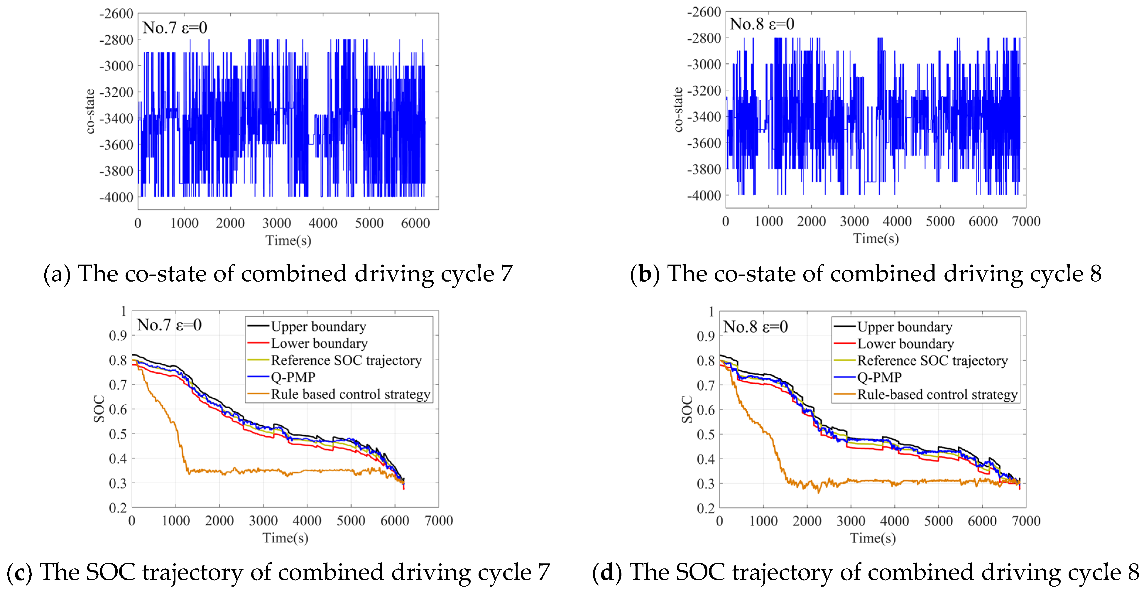
4.2. The Off-Line Verification

To verify the generalization and reliable performances of the Q-Table 6, the combined driving cycle 7 (denoted by No.7) and combined driving cycle 8 (denoted by No.8) are deployed. From Figure 16, it can be seen that the co-state can be well adjusted, based on the driving cycles and the Q-Table 6. Moreover, the final SOCs can satisfy the control object, and the SOC trajectories locate the designed boundary and can easily follow the SOC reference trajectories. This implies that the RL-based strategy has great potential for practical application. In addition, a rule-based energy management is also deployed to evaluate the fuel economy of the RL-based energy management method. From

Table 1. The fuel consumptions of the off-line verification.

Combined Driving Cycle	RL-Based (L/100 km)	Rule-Based (L/100 km)	Fuel Consumption Comparison
No.7	16.8738	18.9497	−10.95%
No.8	16.6673	18.8939	−11.78%

, it can be seen that the fuel consumption of conditions 7 and 8 can be reduced by 10.95% and 11.78%, respectively.

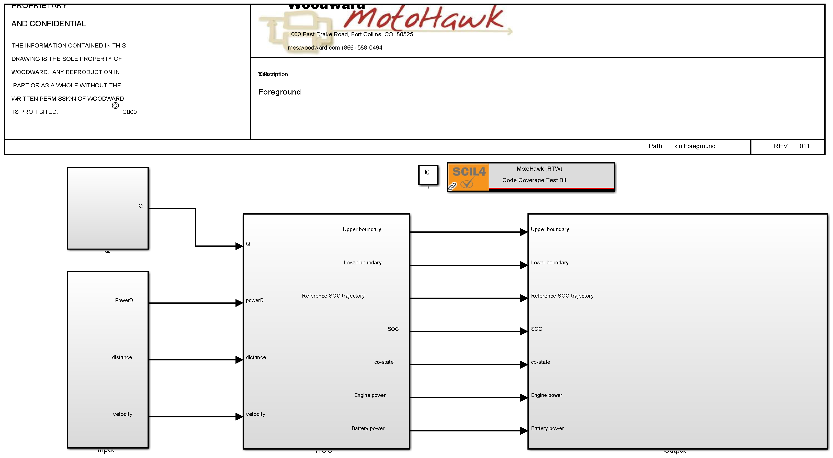
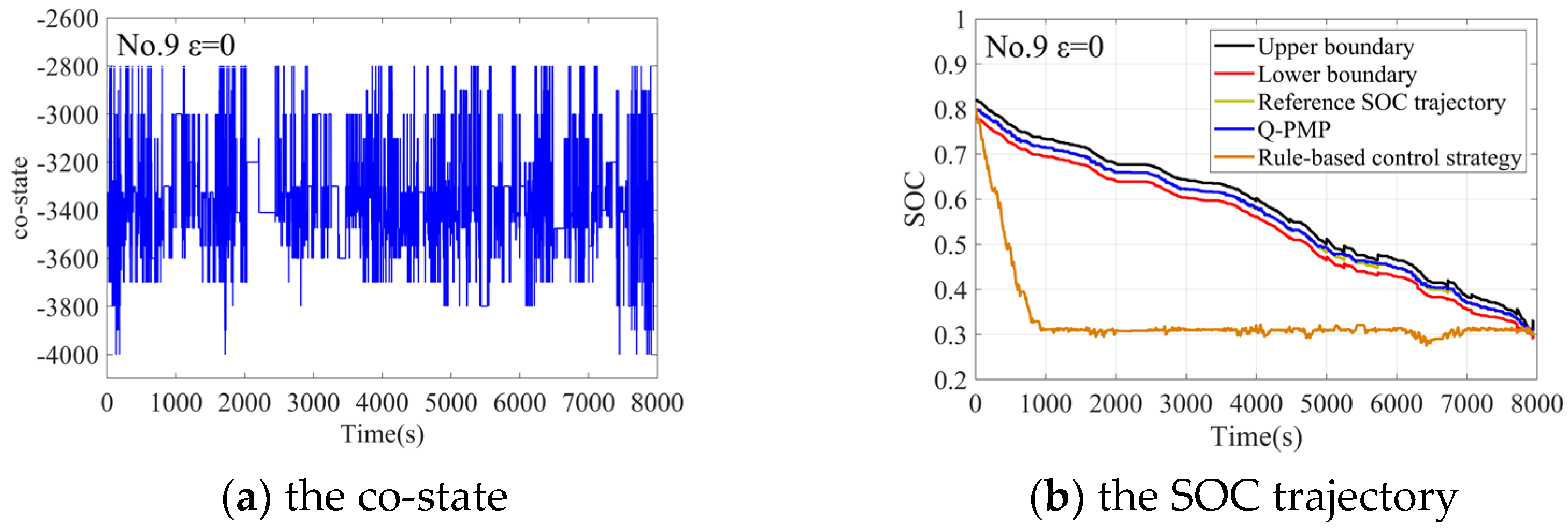
4.3. The Hardware in Loop Simulation Verify

As shown in Figure 17, a HIL test system mainly includes HCU, switch, Upper computer, CAN communication interface, DC 12 V, and Kvaser, built to verify the real-time and reliability of RL-based energy management. Here, the upper computer transmits CAN signals to the HCU through Kvaser.

As shown in Figure 18, a HIL simulation model is built based on D2P rapid prototyping control system and the well trained strategy. It mainly includes three modules: Input, HCU, and Output, where HCU is used to embed the RL-based energy management.

Additionally, the combined driving cycle 9 (denoted by No.9) is also deployed. From Figure 19, it can be seen that the co-state can be adjusted in real-time based on the well-trained strategy, and the control performance can be sufficiently satisfied. Moreover, the fuel consumption can be decreased by 12.92% compared to the rule based strategy as shown in

Table 2. The fuel consumption of the HIL.

Combined Driving Cycle	RL-Based (L/100 km)	Rule-Based (L/100 km)	Fuel Consumption Comparison
No.9	15.2956	17.5642	−12.92%

.

5. Conclusions

This paper proposes an RL-based energy management method based on a novel dynamic SOC design zone plan. The main conclusions are summarized as follows.

Firstly, the proposed dynamic SOC design zone plan method is feasible and applicable. The fuel consumption can be greatly decreased compared to the rule-based energy management.

Secondly, the agent of RL-based energy management can be well trained, and has good generalization performance. Moreover, the trained strategy can be easily embedded into the controller, and the real-time control performance can be satisfied well. It has great potential to be used in practice.

Future work will focus on the further verification of the RL-based energy management in the real vehicles.

References

1. Ajanovic, A.; Haas, R.; Schrödl, M. On the historical development and future prospects of various types of electric mobility. Energies 2021, 14, 1070. [Google Scholar] [CrossRef]
2. Plötz, P.; Moll, C.; Bieker, G.; Mock, P. From lab-to-road: Real-world fuel consumption and CO2 emissions of plug-in hybrid electric vehicles. Environ. Res. Lett. 2021, 16, 054078. [Google Scholar] [CrossRef]
3. Zhang, F.; Hu, X.; Langari, R.; Cao, D. Energy management strategies of connected HEVs and PHEVs: Recent progress and outlook. Prog. Energy Combust. Sci. 2019, 73, 235–256. [Google Scholar] [CrossRef]
4. Huang, Y.; Wang, H.; Khajepour, A.; Li, B.; Ji, J.; Zhao, K.; Hu, C. A review of power management strategies and component sizing methods for hybrid vehicles. Renew. Sustain. Energy Rev. 2018, 96, 132–144. [Google Scholar] [CrossRef]
5. Biswas, A.; Emadi, A. Energy Management Systems for Electrified Powertrains: State-of-The-Art Review and Future Trends. IEEE Trans. Veh. Technol. 2019, 68, 6453–6467. [Google Scholar] [CrossRef]
6. Ding, N.; Prasad, K.; Lie, T.T. Design of a hybrid energy management system using designed rule-based control strategy and genetic algorithm for the series-parallel plug-in hybrid electric vehicle. Int. J. Energy Res. 2021, 45, 1627–1644. [Google Scholar] [CrossRef]
7. Li, P.; Li, Y.; Wang, Y.; Jiao, X. An intelligent logic rule-based energy management strategy for power-split plug-in hybrid electric vehicle. In Proceedings of the 2018 37th Chinese Control Conference (CCC), Wuhan, China, 25–27 July 2018; pp. 7668–7672. [Google Scholar]
8. Hassanzadeh, M.; Rahmani, Z. Real-time optimization of plug-in hybrid electric vehicles based on Pontryagin’s minimum principle. Clean Technol. Environ. Policy 2021, 23, 2543–2560. [Google Scholar] [CrossRef]
9. Wang, W.; Cai, Z.; Liu, S. Study on Real-Time Control Based on Dynamic Programming for Plug-In Hybrid Electric Vehicles. SAE Int. J. Electrified Veh. 2021, 10, 167. [Google Scholar] [CrossRef]
10. Geng, S.; Schulte, T.; Maas, J. Model-Based Analysis of Different Equivalent Consumption Minimization Strategies for a Plug-In Hybrid Electric Vehicle. Appl. Sci. 2022, 12, 2905. [Google Scholar] [CrossRef]
11. Lian, J.; Wang, X.R.; Li, L.H.; Zhou, Y.F.; Yu, S.Z.; Liu, X.J. Plug-in HEV energy management strategy based on SOC trajectory. Int. J. Veh. Des. 2020, 82, 1–17. [Google Scholar] [CrossRef]
12. Liu, Y.J.; Sun, Q.; Han, Q.; Xu, H.G.; Han, W.X.; Guo, H.Q. A Robust Design Method for Optimal Engine Operating Zone Design of Plug-in Hybrid Electric Bus. IEEE Access 2022, 10, 6978–6988. [Google Scholar] [CrossRef]
13. Lin, X.; Zhou, K.; Mo, L.; Li, H. Intelligent Energy Management Strategy Based on an Improved Reinforcement Learning Algorithm With Exploration Factor for a Plug-in PHEV. IEEE Trans. Intell. Transp. Syst. 2021, 1–11. [Google Scholar] [CrossRef]
14. Zhang, H.; Peng, J.; Tan, H.; Dong, H.; Ding, F. A Deep Reinforcement Learning-Based Energy Management Framework With Lagrangian Relaxation for Plug-In Hybrid Electric Vehicle. IEEE Trans. Transp. Electrif. 2020, 7, 1146–1160. [Google Scholar] [CrossRef]
15. Liu, T.; Hu, X.; Hu, W.; Zou, Y. A Heuristic Planning Reinforcement Learning-Based Energy Management for Power-Split Plug-in Hybrid Electric Vehicles. IEEE Trans. Ind. Inform. 2019, 15, 6436–6445. [Google Scholar] [CrossRef]
16. Chen, Z.; Hu, H.; Wu, Y.; Zhang, Y.; Li, G.; Liu, Y. Stochastic model predictive control for energy management of power-split plug-in hybrid electric vehicles based on reinforcement learning. Energy 2020, 211, 118931. [Google Scholar] [CrossRef]
17. Guo, H.Q.; Wei, G.; Wang, F.; Wang, C.; Du, S. Self-Learning Enhanced Energy Management for Plug-in Hybrid Electric Bus With a Target Preview Based SOC Plan Method. IEEE Access 2019, 7, 103153–103166. [Google Scholar] [CrossRef]
18. Qi, C.; Zhu, Y.; Song, C.; Cao, J.; Xiao, F.; Zhang, X.; Xu, Z.; Song, S. Self-supervised reinforcement learning-based energy management for a hybrid electric vehicle. J. Power Sources 2021, 514, 230584. [Google Scholar] [CrossRef]
19. Wu, Y.; Tan, H.; Peng, J.; Zhang, H.; He, H. Deep reinforcement learning of energy management with continuous control strategy and traffic information for a series-parallel plug-in hybrid electric bus. Appl. Energy 2019, 247, 454–466. [Google Scholar] [CrossRef]
20. Tan, H.; Zhang, H.; Peng, J.; Jiang, Z.; Wu, Y. Energy management of hybrid electric bus based on deep reinforcement learning in continuous state and action space. Energy Convers. Manag. 2019, 195, 548–560. [Google Scholar] [CrossRef]
21. He, W.; Huang, Y. Real-time Energy Optimization of Hybrid Electric Vehicle in Connected Environment Based on Deep Reinforcement Learning. IFAC-PapersOnLine 2021, 54, 176–181. [Google Scholar] [CrossRef]
22. Kim, N.; Jeong, J.; Zheng, C. Adaptive energy management strategy for plug-in hybrid electric vehicles with Pontryagin’s minimum principle based on daily driving patterns. Int. J. Precis. Eng. Manuf.-Green Technol. 2019, 6, 539–548. [Google Scholar] [CrossRef]
23. Xie, S.; Hu, X.; Xin, Z.; Brighton, J. Pontryagin’s minimum principle based model predictive control of energy management for a plug-in hybrid electric bus. Appl. Energy 2019, 236, 893–905. [Google Scholar] [CrossRef] [Green Version]
24. Guo, H.; Du, S.; Zhao, F.; Cui, Q.; Ren, W. Intelligent Energy Management for Plug-in Hybrid Electric Bus with Limited State Space. Processes 2019, 7, 672. [Google Scholar] [CrossRef] [Green Version]
25. Guo, H.; Zhao, F.; Guo, H.; Cui, Q.; Du, E.; Zhang, K. Self-learning energy management for plug-in hybrid electric bus considering expert experience and generalization performance. Int. J. Energy Res. 2020, 44, 5659–5674. [Google Scholar] [CrossRef]
26. Onori, S.; Tribioli, L. Adaptive Pontryagin’s Minimum Principle supervisory controller design for the plug-in hybrid GM Chevrolet Volt. Appl. Energy 2015, 147, 224–234. [Google Scholar] [CrossRef]
Figure 1. The structure of the PHEB.
Processes 10 01080 g001
Figure 2. The fuel consumption rate MAP of the engine.
Processes 10 01080 g002
Figure 3. The efficiency MAP of the motor.
Processes 10 01080 g003
Figure 4. The Rint model of the battery.
Processes 10 01080 g004
Figure 5. The principle of the dynamic SOC design zone method.
Processes 10 01080 g005
Figure 6. The principle of the reinforcement learning.
Processes 10 01080 g006
Figure 7. The principle of the RL-based energy management.
Processes 10 01080 g007
Figure 8. The design process of the RL-based energy management.
Processes 10 01080 g008
Figure 9. The combined driving cycles.
Processes 10 01080 g009
Figure 10. The training process of combined driving cycle 1.
Processes 10 01080 g010
Figure 11. The training process of combined driving cycle 2.
Processes 10 01080 g011
Figure 12. The training process of combined driving cycle 3.
Processes 10 01080 g012
Figure 13. The training process of combined driving cycle 4.
Processes 10 01080 g013
Figure 14. The training process of combined driving cycle 5.
Processes 10 01080 g014
Figure 15. The training process of combined driving cycle 6.
Processes 10 01080 g015
Figure 16. Offline verification results of combined driving cycles 7 and 8.
Processes 10 01080 g016
Figure 17. The HIL test system.
Processes 10 01080 g017
Figure 18. The composition of HIL.
Processes 10 01080 g018
Figure 19. The HIL test results of combined driving cycle 9.
Processes 10 01080 g019