Article

Research on the Desired Dynamic Selection of a Reference Model-Based PID Controller: A Case Study on a High-Pressure Heater in a 600 MW Power Plant

1
State Key Lab of Power Systems, Department of Energy and Power Engineering, Tsinghua University, Beijing 100084, China
2
School of Electrical Engineering, Zhengzhou University, Zhengzhou 450001, China
3
Institute of Gas Turbines, Department of Energy and Power Engineering, Tsinghua University, Beijing 100084, China
*
Author to whom correspondence should be addressed.
Processes 2022, 10(6), 1059; https://doi.org/10.3390/pr10061059
Submission received: 8 May 2022 / Revised: 20 May 2022 / Accepted: 23 May 2022 / Published: 25 May 2022
(This article belongs to the Section Process Control and Monitoring)

Abstract

:
Nowadays, the proportional–integral–derivative (PID) controller dominates industrial process control. Because of the compromise between parameters, its tuning is still a challenge for practitioners. A reference model (RM)-based PID controller—the desired dynamic equational (DDE) PID controller—is regarded as a viable alternative since it can readily eliminate the compromise. However, how to design its desired dynamic equation remains an unsolved problem which limits the application of DDE PID controllers in large-scale industrial systems. Therefore, this paper studies the desired dynamic selection of DDE PID controllers and proposes a simple and practical selection procedure without using the accurate plant model. Simulations, experiments and filed tests demonstrate the convenience and advantages of the proposed method, thus making DDE PID an effective controller type which is specifically appealing to engineers. Moreover, the successful application of DDE PID controllers to a high-pressure (HP) heater in a coal-fired power plant shows their promising prospects in the future power industry with the increasing demand to integrate more renewables into the grid.

1. Introduction

Nowadays, coal-fired power plants dominate the worldwide power supply, particularly in China [1]. In 2020, coal-fired generation occupied 65% of the Chinese total generation, although renewable energy such as wind and solar power have developed rapidly in recent years [2]. Because of the increasing power demand and the randomness of renewable energies, thousands of coal-fired units participate in deep peak shaving by frequently regulating the output power according to automatic generation command (AGC). Therefore, it is of importance that all control loops respond to AGC in the shortest time, which requires fast and moderate reference tracking performance by all controllers.
The proportional–integral–derivative (PID) controller [3] still remains as the first choice for thermal engineers, although advanced control strategies, such as model predictive control (MPC) [4,5] and active disturbance rejection control (ADRC) [6,7,8,9,10,11], have been attempted to be widely applied to the control systems of coal-fired power plants in the past decades. It has the superiorities of a simple structure and reliable performance, so it plays a significant role in the control of thermal processes. According to a survey conducted in more than 100 boiler turbine units in Guangdong Province, China, the traditional PI or PID controller is applied to about 98% of feedback loops in coal-fired power plants [12]. Since its wide applications in industrial process control systems, researchers worldwide have been studying the engineering tuning method of the PI or PID controller for a long time to achieve satisfactory performance [13]. Most of the classical tuning methods are summarized in a handbook [14] for different industrial processes, such as the Ziegler–Nichols (Z-N) method [15], internal model control (IMC) method [16], Skogestad IMC (SIMC) method [17], Ms-constrained integral gain optimization (MIGO) method [18,19], and so forth, which provides guidance on PID tuning for thermal engineers. Moreover, some intelligence and optimization algorithms are combined with the PI or PID design, including fuzzy control [20,21], the genetic algorithm (GA) [22], extremum seeking (ES) [23], particle swarm optimization [24], and so forth, whose superiorities in reference tracking have been validated by simulations. However, the applications of the aforementioned PID tuning or design methods are limited in the control system of the coal-fired unit because of the following:
  • Using most engineering tuning methods, such as the Z-N method, the closed-loop response may exhibit a large overshoot and long settling time, which brings potential challenges to the longevity of the actuator and the safe operation of the unit [25];
  • Plant model-based tuning methods need a time-consuming identification process and will obtain poor performance when the model is mismatched [26];
  • Only simple control algorithms, such as integral and derivative, can be implemented on the distributed control system (DCS) [27].
A reference model (RM)-based PID controller synthesis method—desired dynamic equational (DDE) PID [28,29], which was previously developed by the authors—is regarded as a viable alternative to PID design in thermal engineering. Its core idea is that the parameters of the controller are relative to the coefficients of the desired dynamic equation. When the PI or PID controller is tuned appropriately, the closed-loop output will track the response of the typical first- or second-order system accurately. Up to now, the superiorities of DDE PI or PID, such as fast and moderate tracking performance, strong disturbance rejection ability and simple tuning procedure, have been validated only by numerical simulations [30,31,32,33,34,35] and not industrial field tests.
However, the feedback control system has its inherent limitations when dealing with uncertainties [36,37], which means that its response speed is unable to be infinitely fast. As a result, if the desired dynamic equation is designed inappropriately, the performance of the closed-loop system will deteriorate. For example, the overly quick desired dynamic response of DDE PI or PID controller may lead to severe oscillation of the closed-loop output or actuator saturation, which brings challenges to the safe operation of a unit. Unfortunately, how to select the appropriate desired dynamic equation for DDE PI or PID has not received enough attention, although it is worthy of studying. Based on this motivation and keeping simplicity in mind, this paper studies the desired dynamic selection of DDE PI or PID. The main contributions of this paper are as follows:
  • A practical selection procedure of the desired dynamic equation of DDE PI or PID is summarized without using accurate plant models for practitioners;
  • Based on the proposed selection procedure, DDE PI is first applied to the control of a practical thermal process: the level of a high-pressure (HP) heater in a 600-MW coal-fired power plant.
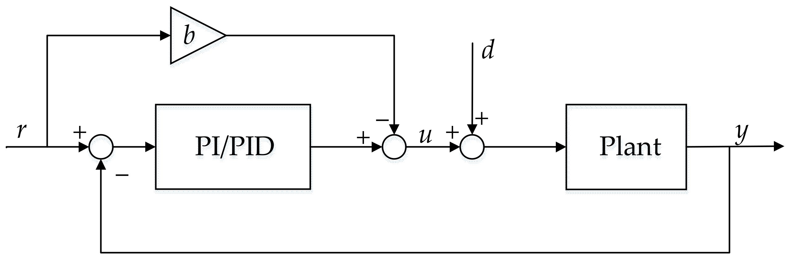
The rest of this paper is organized as follows. The principle of DDE PI or PID is introduced in Section 2. Based on the influence of the parameters of DDE PI or PID on the control performance analyzed in Section 3, the selection procedure of the desired dynamic equation is summarized in Section 4, and its effectiveness is demonstrated by several illustrative examples in Section 5. Moreover, experiments on the water tank and field tests on the HP heater indicate the applicability and superiorities of the DDE PI or PID controller designed based on the proposed method in Section 6 and Section 7, respectively. Finally, the concluding remarks are presented in the last section.

2. DDE PI or PID

Consider the transfer function model of a general system depicted as
G p s = H a 0 + a 1 s + + a m n 1 s m n 1 + s m n b 0 + b 1 s + + b m 1 s m 1 + s m e τ s ,
where ai (i = 1, 2, ⋯, mn − 1) and bj (j = 1, 2, ⋯, m − 1) are defined as coefficients of the numerator and the denominator, respectively. Aside from that, m, n, τ and H are denoted as the order of the denominator, the relative degree, the delay time and the high frequency gain, respectively. Note that ai (i = 1, 2, ⋯, mn − 1), bj (j = 1, 2, ⋯, m − 1) and H are usually unknown.
According to the description of the general system in [38], the following assumptions are proposed:
  • The relative degree n is known;
  • The general system is a minimum-phase plant;
  • The sign of the high-frequency gain H is known;
  • The denominator and the numerator of the general system are relatively prime, and the unobservable and uncontrollable modes are asymptotically stable.
The general system depicted in Equation (1) can be transformed to the normalized state-space form as
x ˙ i = x i + 1 ,                                                                                                                         i = 1 , , n 1 x ˙ n = i = 0 n 1 λ i x i + 1 i = 0 m n 1 ζ i w i + 1 + H u w ˙ i = w i + 1 ,                                                                                                                         i = 1 , , m n 1 w ˙ m n = i = 0 m n 1 a i w i + 1 + x 1 y = x 1 ,
where λi (i = 0, 1, ⋯, n − 1) and ζi (i = 0, 1, ⋯, mn − 1) are unknown parameters while xi (i = 1, 2, ⋯, n − 1) and wi (i = 1, 2, ⋯, mn − 1) are the state-space variables and uncertainties, respectively. If an extended state f is defined as
f x , w , u = i = 0 n 1 λ i x i + 1 i = 0 m n 1 ζ i w i + 1 + H l u   ,
where l is the estimated value of H, then in Equation (2), x ˙ n can be rewritten as
x ˙ n = f + l u ,
If n = 2, which means that the plant can be regarded as a general second-order system, the state-space model of the general system is depicted as follows:
x ˙ 1 = x 2 x ˙ 2 = f + l u y = x 1 ,
Correspondingly, if the closed-loop desired dynamic equation is designed such that
y ¨ + h 1 y ˙ + h 0 = h 0 r ,
where r is denoted as the set point, and h0 and h1 are defined as the coefficients of the desired dynamic equation, then to eliminate f, the control law should be designed as follows:
u = h 0 r z 1 h 1 z 2 f ^ l ,
where z1 = x1, z2 = x2 and f ^ is the estimation of f, which can be estimated by following the disturbance observer algorithm:
ξ ˙ = k ξ k 2 z 2 k l u f ^ = ξ + k z 2 ,
In Equation (8), k and ξ are denoted as the gain and the intermediate state variable of the disturbance observer, respectively. Combined with Equation (7), the control law can be rewritten as
u = ξ + k z 2 l h 0 z 1 r + h 1 z 2 l ,
According to Equations (8) and (9), the derivative of the intermediate variable is derived as follows:
ξ ˙ = k h 0 z 1 r + h 1 z 2 ,
By integrating both sides of Equation (10), it is evident that
ξ = k h 0 z 1 r d t + h 1 z 1 ,
Combined with Equation (9), the control law can be rewritten as
u = k h 0 z 1 r d t + h 1 z 1 + k z 2 l h 0 z 1 r + h 1 z 2 l = h 0 + k h 1 l r z 1 + k h 0 l r z 1 d t h 1 + k l z 2 k h 1 l r
Due to that, r is the step change in practical processes and r ˙ is unbounded and can be set as zero [39]. By defining the error between the set point and the output as e = rz1, it is easy to obtain that e ˙ = r ˙ z ˙ 1 = z 2 . As a result, Equation (12) can be rewritten as
u = h 0 + k h 1 l e + k h 0 l e d t + h 1 + k l e ˙ k h 1 l r       = k p e + k i e d t + k d e ˙ b r
From Equation (13), it is obvious that DDE PID is a type of two-degree-of-freedom (TDOF) PID controller with reference feedforward, and kp, ki, kd and b are denoted as the proportional, integral, derivative and the feedforward gains, respectively.
Similarly, if n = 1, which means that the plant is considered a general first-order system, the desired dynamic equation can be designed as h0/(s + h0). Correspondingly, the control law of DDE PI can be achieved based on the same derivation of Equations (5)–(13):
u = h 0 + k l e + k h 0 l e d t k l r       = k p e + k i e d t b r
Based on Equations (13) and (14), the structure of DDE PI/PID is illustrated in Figure 1. Note that d is denoted as the external disturbances.
Stability analysis is of significance for a controller. In terms of the linear time invariant (LTI) system, the closed-loop stability can be analyzed based on the Routh–Hurwitz criterion [40]. However, most thermal processes in a coal-fired power plant are nonlinear, time-variant, distributed parametrically and have uncertainties. As a result, the Routh–Hurwitz criterion is inapplicable for the stability analysis of DDE PID.
In this paper, the asymptotic stability of DDE PID is analyzed based on Lyapunov’s method [41]. The details are presented in Appendix A.

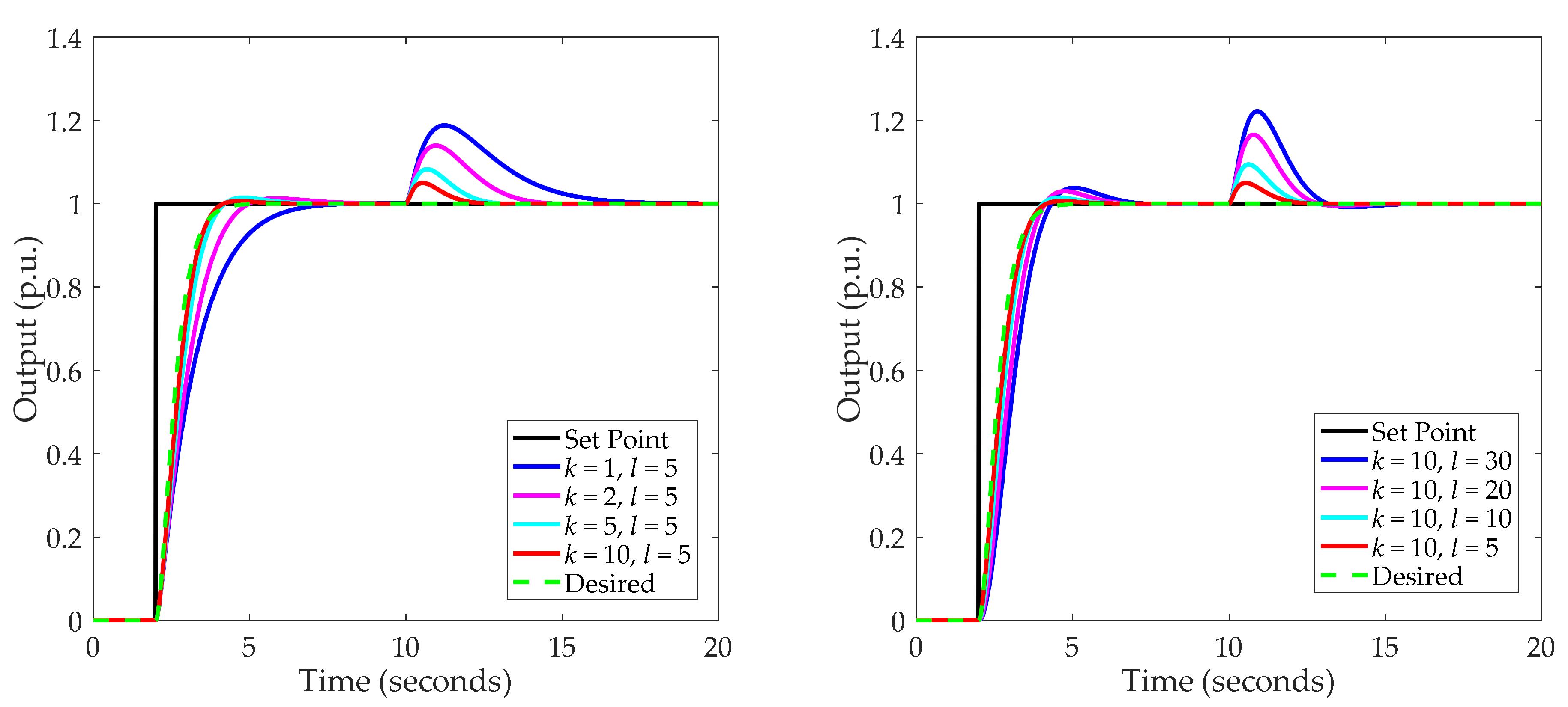
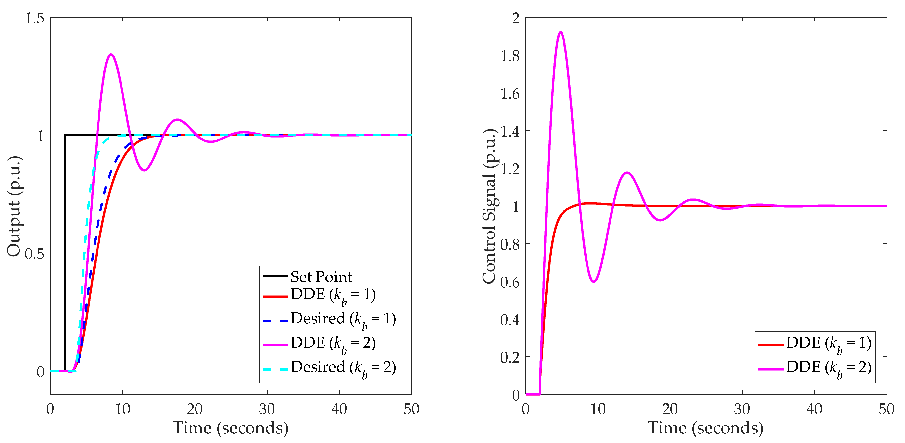
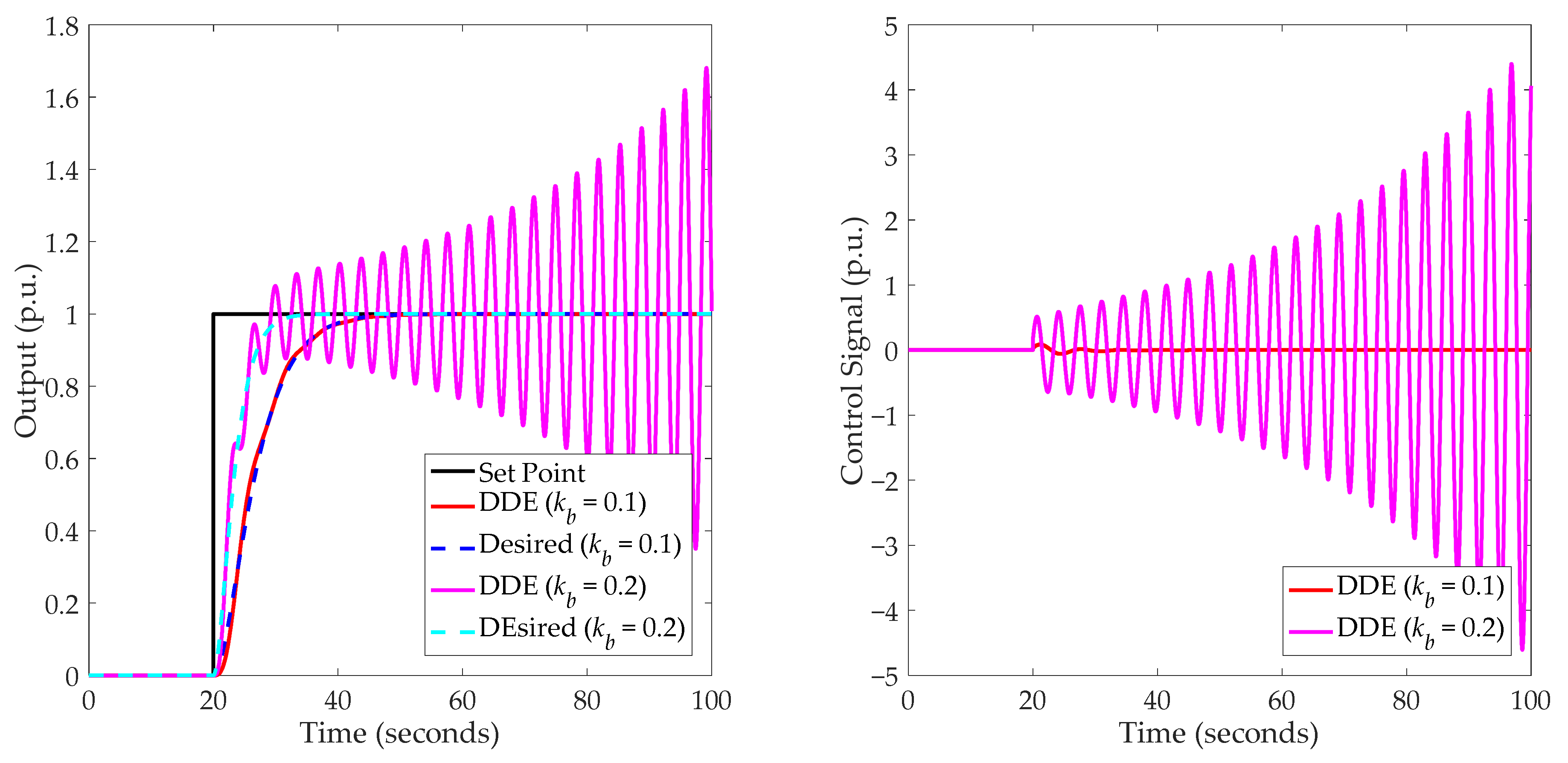
3. The Influence of Parameters of DDE PI or PID on Control Performance

To summarize the selection procedure of the desired dynamic equation, it is necessary to analyze the influence of the parameters of DDE PI or PID on the control performance. The desired dynamic equation of DDE PI or PID is rewritten as follows to reduce the number of tunable parameters:
h 0 s + h 0 = ω d s + ω d                                   DDE   PI h 0 s 2 + h 1 s + h 0 = ω d 2 s + ω d 2             DDE   PID ,
where ωd is defined as the desired closed-loop bandwidth in this paper. If the plant has a pure time delay, the desired dynamic equation should be designed as in Equation (16) since the time delay is unavoidable [42]:
ω d s + ω d e τ s                                   DDE   PI ω d 2 s + ω d 2 e τ s                           DDE   PID ,
According to Equations (13)–(16), it is obvious that the tunable parameters of DDE PI and PID are k, l and ωd. In terms of ωd, it determines the speed of the desired dynamic equation, whose selection procedure will be discussed in the next section. As for k and l, they are tuned to let the output track the desired dynamic response precisely.
In this section, the influence of k and l on the control performance of DDE PID is analyzed. First, the following propositions are proven:
Proposition 1. 
When k→∞, the closed-loop system with DDE PID will follow the characteristics of Equation (6).
Proof. 
By defining f ˜ = f ^ f , then
f ˜ ˙ t = f ^ ˙ f ˙                   = ξ ˙ + k z ˙ 2 f ˙                   = k ξ + k 2 z 2 k l u + k f + k l u f ˙                   = k ξ + k z 2 + k f f ˙                   = k f ˜ f ˙
Construct the Lyapunov function V1(t) as follows:
V 1 t = 1 2 f ˜ t 2 ,
Therefore, the following is true:
V ˙ 1 t = f ˜ ˙ f ˜ = k f ˜ 2 f ˜ f ˙ k f ˜ 2 + f ˙ 2 V 1 t = 2 k V 1 t + f ˙ 2 V 1 t ,
Assume that f ˙ is bounded and f ˙ < M . As a result, Equation (19) satisfies the following:
V ˙ 1 t 2 k V 1 t + 2 M V 1 t ,
From Equation (20), it is derived that
d V 1 t d t = V ˙ 1 t 2 V 1 t                         = 1 2 V 1 t 2 k V 1 t + 2 M V 1 t                         = k V 1 t + 2 2 M
For all tt0, which yields further, then
0 V 1 t e k t V 1 t 0 + 2 2 M t 0 t e k t τ d τ 0 lim t V 1 t lim t e k t V 1 t 0 + 2 2 M t 0 t e k t τ d τ
When k→∞, lim t V 1 t = 0 , which means that f ^ f 0 , then Equation (7) can be rewritten as
u k h 0 r z 1 h 1 z 2 f l ,
Therefore, Equation (5) can be written as
x ˙ 2 = f + l u         = f + l h 0 r z 1 h 1 z 2 f l         = h 0 r z 1 h 1 z 2
Since z1 = x1 and z2 = x2, Equation (24) can be depicted as follows:
x ˙ 2 = h 0 r x 1 h 1 x 2 y ¨ = h 0 r y h 1 y ˙
As a result, the closed-loop system with DDE PID will follow the characteristics of Equation (6) when k→∞.   □
Proposition 2. 
If k is sufficiently large, the closed-loop system with DDE PID will follow the characteristics of Equation (6) when l→0.
Proof. 
From Equation (5), it is evident that x ˙ 2 f when l→0. That aside, according to Equation (6), it is obvious that
f ^ l 0 k s + k z ˙ 2 ,
Since k is sufficiently large, it is assumed that f ^ z ˙ 2 = x ˙ 2 when l→0, which means that f ^ f . Then, based on Equations (24) and (25), it can be derived that the closed-loop system with DDE PID will follow the characteristics of Equation (6) when l→0.   □
On the basis of Propositions 1 and 2, the following remark can be summarized:
Remark 1. 
With the increase in k or the decrease in l, the closed-loop DDE PID will be closer to the desired dynamic response.
Remark 1 can be validated by an illustrative example. Consider a simple second-order system whose transfer function model is depicted as 1 s + 1 0 . 2 s + 1 , and ωd is set as 1. Figure 2 shows the influence of k and l on the control performance of DDE PID. Note that l is fixed at 5 when k is varying from 1 to 10, while k is fixed at 10 when l is tuning from 30 to 5. Aside from that, a step disturbance was added during the simulations.
According to Figure 2, it is obvious that Remark 1 was demonstrated by the simulations. In addition, larger k values and smaller l values mean better disturbance rejection performance.

4. The Desired Dynamic Selection of DDE PI and PID

4.1. The Initialization of Controller Parameters

The initial values of DDE PI and PID are necessary to evaluate because they are used to start the selection procedure. Therefore, in this subsection, the calculations of the initial values of k, l and ωd are discussed.
It was mentioned in Section 2 that the thermal processes in the coal-fired power plants are difficult to model accurately. When the unit is running, only the open-loop step response of the process is available for the design and tuning of the controller. As a result, the initial values of the parameters should be evaluated based on the open-loop response of the process. Figure 3 shows the open-loop step responses of the processes.
In Figure 3, tstep, A, A0, y0 and y are denoted as the step time, the initial value and amplitude of the step response and the initial value and stable value of the output, respectively. Moreover, a time variable, the response time of the process, is defined as tp, which is used to describe the time scale of the process. It is easy to evaluate according to the illustrations in Figure 3.
First, the initial value of ωd is studied. The closed-loop desired bandwidth determines the time scale of the desired dynamic equation, which should be evaluated based on the time scale of the process. In this paper, the initial desired dynamic equation is designed to have the same response time as the process, which means that the initial ωd should be calculated as follows:
ω d 0 = 3.91 / t p τ   DDE   PI 5.84 / t p τ   DDE   PID ,
where ωd0 refers to the initial ωd.
Second, the initial value of k is evaluated. According to Equation (26), it can be derived that f ^ = k s + k f . Therefore, k determines the pole of the equivalent disturbance observer. For the observer design, the trade-off between the time required to obtain accurate observer performance and the amount of noise amplification is a primary design issue, so a separation of the desired closed-loop system poles (ωd) and the observer poles (k) to an order from 2 to 10 should be insured [43]. To obtain better observer performance, in this paper, let k = 10ωd according to Remark 1. As a result, the initial value of k, denoted as k0, should be set to 10ωd0.
Finally, the initial value of l is discussed. It was mentioned in Section 2 that l is the estimation of H. However, H is usually unknown. According to Equation (2), H is relative to the critical gain, which is defined as the gain between x ˙ 1 or x ˙ 2 and u for DDE PI and PID. Correspondingly, the initial value of l should be set based on the critical gain.
Denote the critical gain as l ˜ , and it can be evaluated as follows.
In terms of DDE PI, the step responses of open-loop stable and unstable systems can be approximated as those of systems depicted as in Equation (28) by the tangent method or two-point approximation method [44]:
G p s K T s + 1 e τ s             Open - loop   Stable   System K s e τ s                     Open - loop   Unstable   System ,
where K and T are denoted as the gain and the time constant, respectively. Then, the critical gain can be calculated by
l ˜ = K / T           Open - loop   Stable   System K                     Open - loop   Unstable   System ,
As for DDE PID, the step responses of open-loop stable and unstable systems can be approximated as those of systems depicted as in Equation (30) by the two-point approximation method [45]:
G p s K T 1 s + 1 T 2 s + 1 e τ s                 Open - loop   Stable   System K s T 2 s + 1 e τ s                                 Open - loop   Unstable   System ,
where T1 and T2 are known as the time constants of the approximated second-order system. Therefore, the critical gain can be calculated by
l ˜ = K / T 1 T 2           Open - loop   Stable   System K / T 2                           Open - loop   Unstable   System ,
Note that the derivation of the critical gain is detailed in Appendix B. According to [29], a larger l means a wider stable region of DDE PI or PID. As a result, to avoid the immediate non-convergence of the closed-loop system, the initial value of l, l0, is recommended to be set to 10 l ˜ for a larger stable margin.
According to the initialization of DDE PI and PID, it can be concluded that all controller parameters have their own physical meanings; that is, ωd, k and l are related to the time scale of the process, the observer bandwidth and the gain, respectively. As a result, the tuning of DDE PI and PID is easier to understand for engineers than other PID tuning methods.

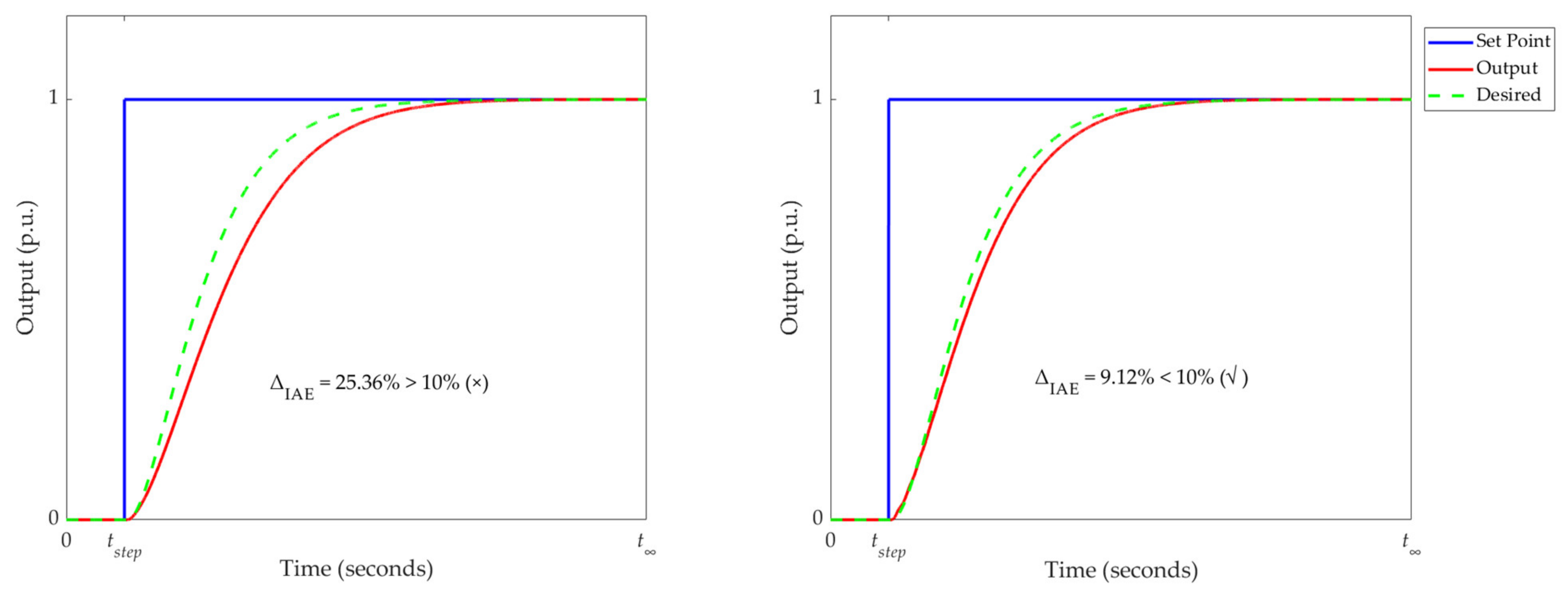
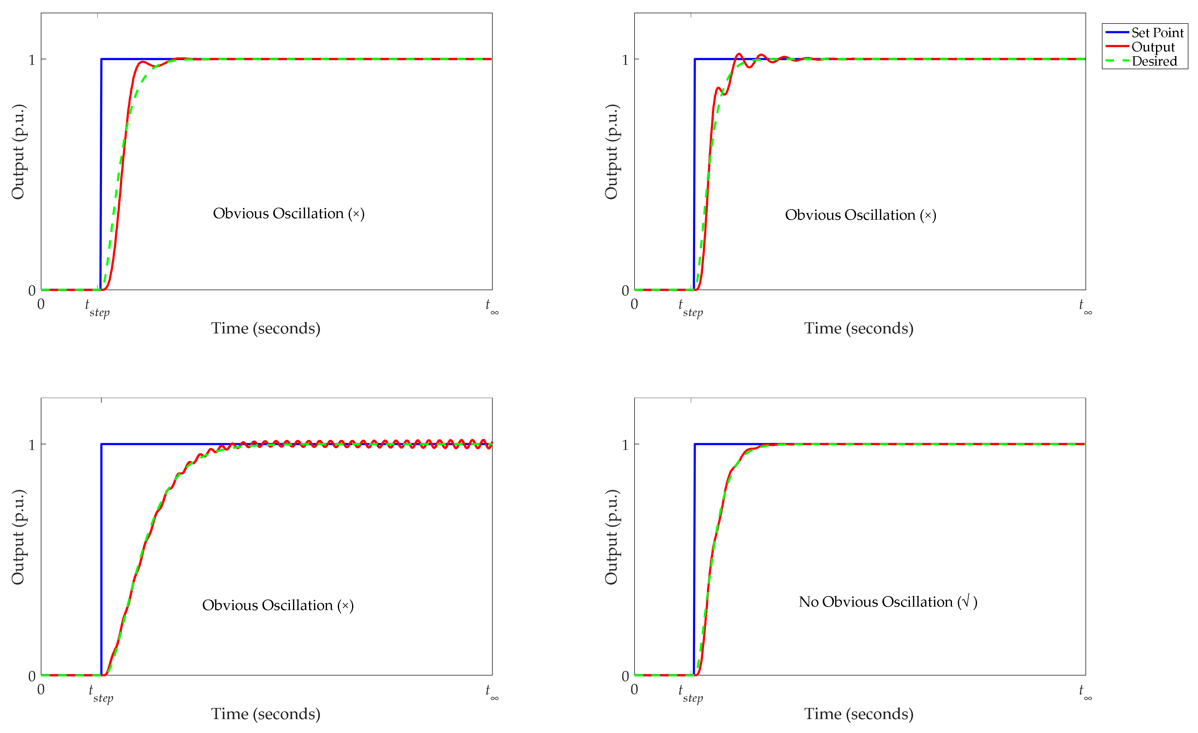
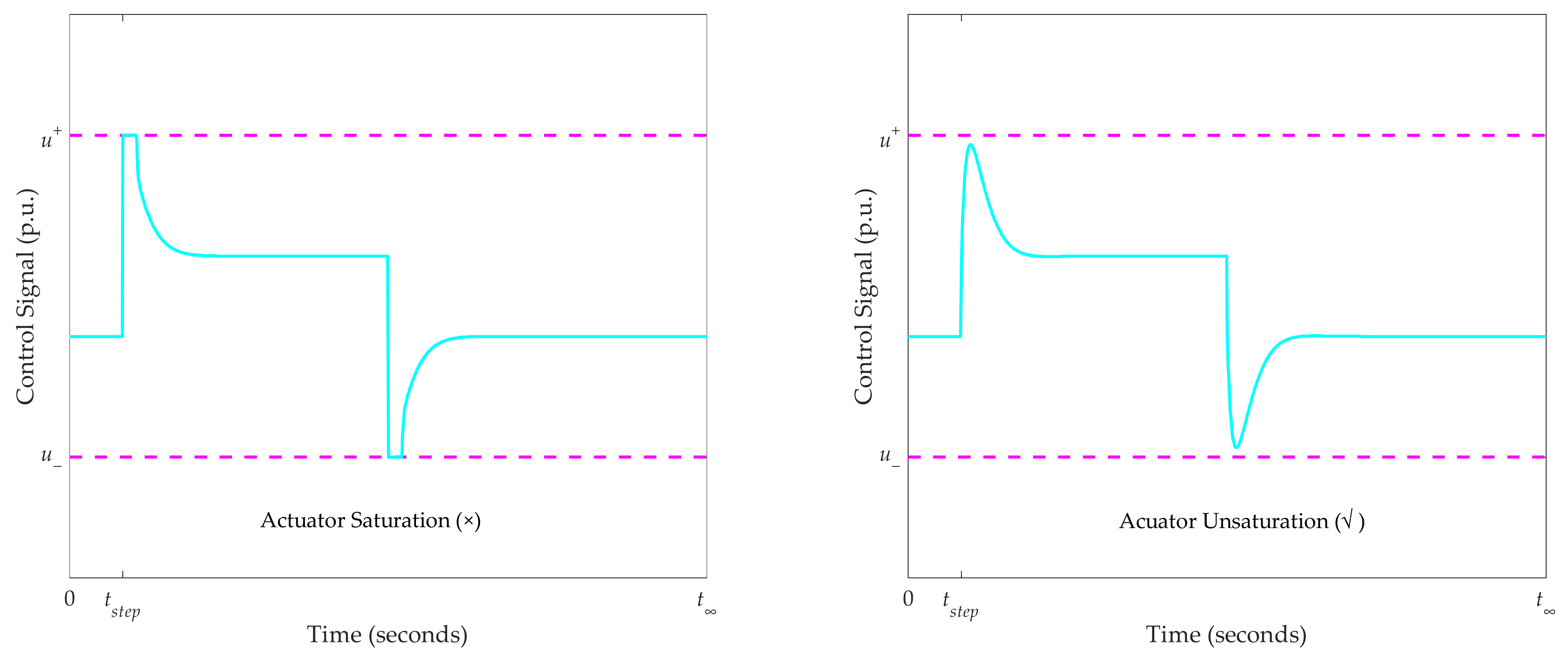
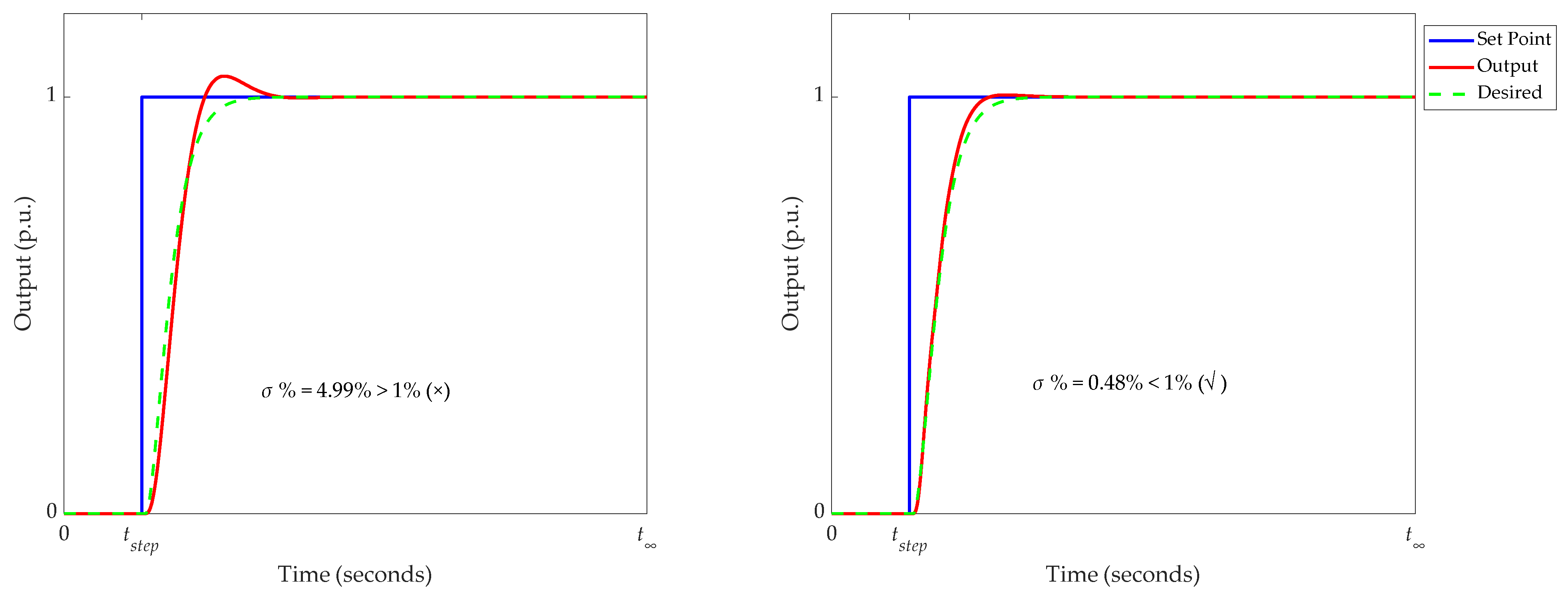
4.2. The Criteria of Tracking the Desired Dynamic Response

According to Proposition 1, it is easy to learn that the closed-loop output will follow the characteristics of the desired dynamic equation when the total disturbance f is completely compensated. However, f is usually unmeasurable in practice and unable to be totally eliminated. Hence, it is difficult to theoretically judge whether the closed-loop output has tracked the desired dynamic response accurately by evaluating the compensation of the total disturbance.
Taking simplicity into account, four criteria for tracking the desired dynamic response are suggested for practitioners, and they are as follows. When the closed-loop stability is guaranteed, the output is considered to be tracking the desired dynamic response accurately if all criteria are satisfied in this paper:
Criterion 1. 
The error of the integral absolute error (IAE) between the closed-loop output and the desired dynamic response is no larger than 10%.
A new index to evaluate the IAE between two responses, ΔIAE, is defined as follows:
Δ IAE = IAE p IAE d IAE d × 100 % ,
where IAEp is denoted as the IAE between r and y, while IAEd refers to the IAE between r and the desired dynamic response (yd). In this paper, it is required that ΔIAE ≤ 10%. However, the criterion is flexible, as it changes with the control requirements. For example, if the requirement is stricter, ΔIAE can be set no larger than 5%. Figure 4 shows an illustration of Criterion 1.
In this article, t is denoted as the stop time of the simulation or the experiment:
Criterion 2. 
The overshoot of the closed-loop output should be lower than 1%.
The desired dynamic response is the response of a typical first-order or second-order plus delay time (FO/SOPDT) system, which has moderate tracking performance. As a result, a significant overshoot is undesirable. In this paper, the overshoot, denoted as σ%, is desired to be lower than 1%. Similar to Criterion 1, this criterion is flexible as well. Figure 5 shows an illustration of Criterion 2.
Criterion 3. 
The closed-loop output has no obvious oscillation.
Due to inappropriate controller parameters, the closed-loop output may exhibit obvious oscillation even though the closed-loop stability is guaranteed, and the overshoot is smaller than 1%. For moderate control performance, obvious oscillation should be avoidable. However, this criterion is qualitative, so it should be judged by practitioners whether the oscillation is obvious. Figure 6 presents an illustration of Criterion 3.
From Figure 6, when there is obvious oscillation, both Criterion 1 and Criterion 2 are satisfied. Nevertheless, the closed-loop output is unable to be regarded as tracking the desired dynamic response accurately.
Criterion 4. 
The actuator should be unsaturated.
The saturations of the actuator, including the amplitude limits and rate limits, are necessary to consider for the tuning of the controller. Larger parameters for the controller mean stronger control action, which may lead to amplitude saturation and further shorten the longevity of the actuator [46]. Therefore, saturations should be avoided during the tuning of DDE PI and PID to protect the actuator. Figure 7 shows an illustration of Criterion 4.
In Figure 7, u+ and u are denoted as the upper and lower limits of the actuator, respectively.

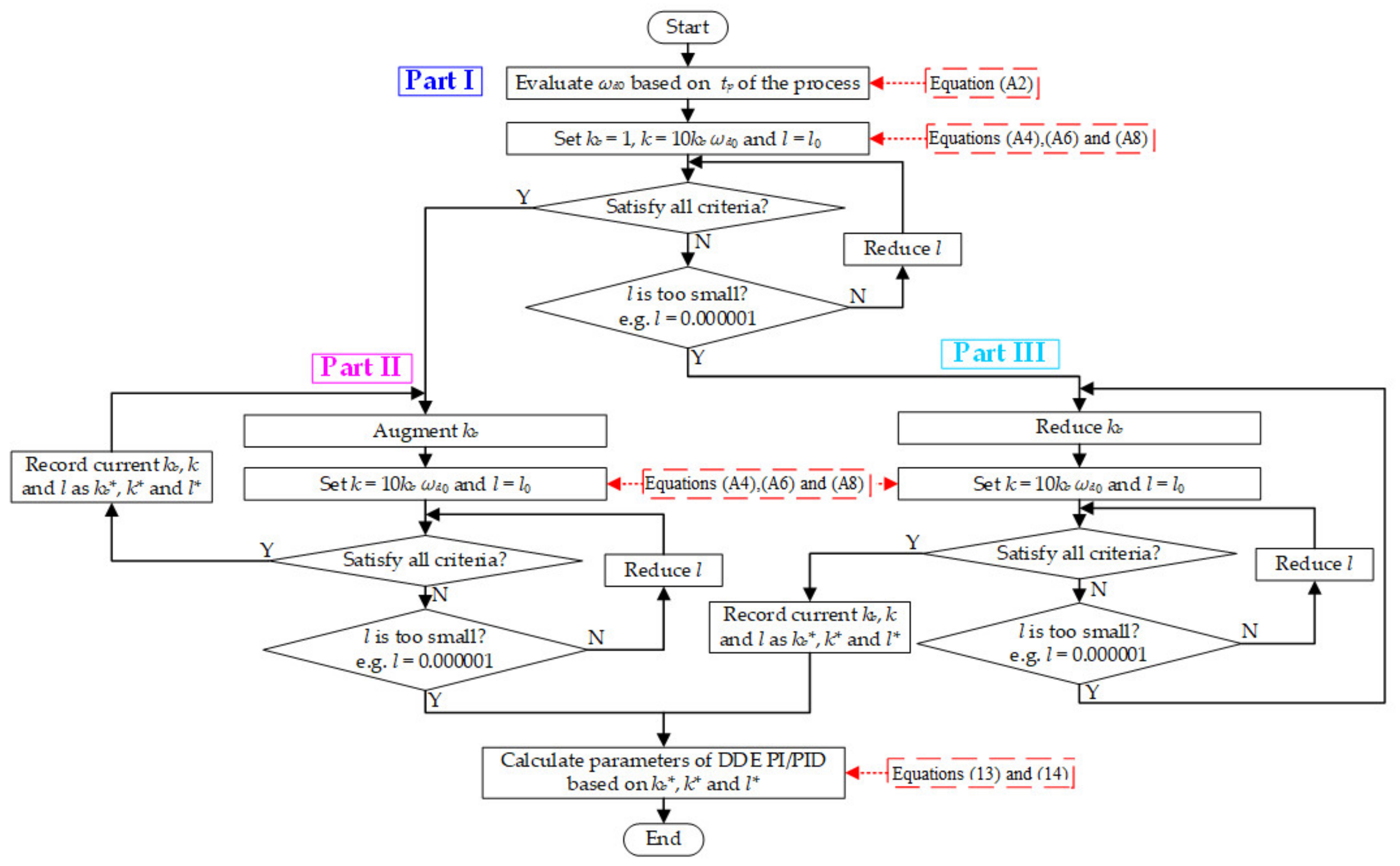
4.3. The Selection Procedure of the Desired Dynamic Equation

The desired dynamic selection procedure proposed in this subsection can be regarded as a tuning method of DDE PI or PID to achieve following goals under the constraints of the actuator and the plant:
  • The reference tracking speed is as fast as possible;
  • The closed-loop output tracks the desired dynamic response accurately.
In this section, a new parameter is defined, kb, which is depicted as follows:
ω d = k b ω d 0 ,
From Equation (33), it is obvious that kb is used to evaluate the multiple relationships between the speed of the current desired dynamic response and that of the initial one.
Generally, the design of DDE PI or PID for the thermal processes of coal-fired power plants can be summarized as the following steps:
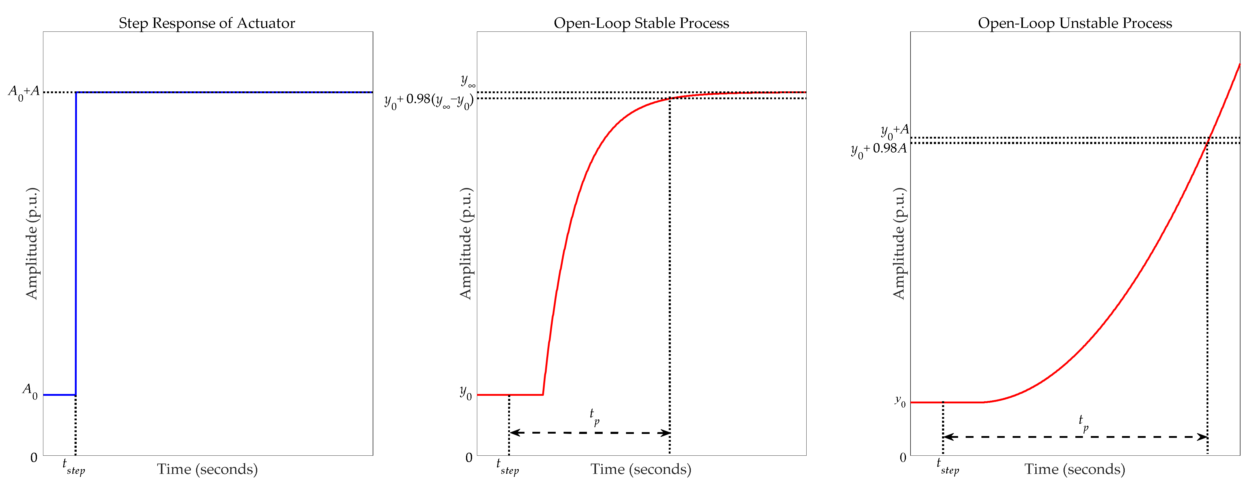
  • Obtain the gain and the time scale of the process based on the open-loop test;
  • Calculate the initial values of the parameters of DDE PI or PID;
  • Tune DDE PI or PID based on the proposed desired dynamic selection procedure.
The selection procedure can be divided into following three parts:
Part I. First, it is necessary to judge whether the closed-loop output of DDE PI or PID can track the initial desired dynamic response accurately by tuning the parameters of the controller. According to Section 4.1, the initial desired dynamic response can be determined based on tp of the process. Based on the analysis in Section 3, the step-by-step procedure of Part I can be summarized as follows:
  • Step 1: Evaluate ωd0 based on the tp of the process according to Equation (27);
  • Step 2: Set kb = 1, k = 10kbωd0 and l = l0;
  • Step 3: Judge whether all criteria are satisfied. If satisfied, terminate the procedure of Part I and turn to that of Part II. If not, proceed to Step 4;
  • Step 4: Judge whether l is too small (e.g., l = 0.000001). If l is too small, terminate the procedure of Part I and turn to that of Part III. If not, reduce l and go back to Step 3.
Part II. Second, the procedure of Part I terminating at Step 4 means that the desired dynamic response can be set faster than the initial one. Therefore, ωd should be augmented until all criteria are unable to be satisfied by tuning the parameters of DDE PI or PID.
The step-by-step procedure of Part II can be summarized as follows:
  • Step 1: Augment kb;
  • Step 2: Set k = 10kbωd0 and l = l0;
  • Step 3: Reduce l;
  • Step 4: Judge whether all criteria are satisfied. If satisfied, record the current kb, k and l as kb*, k* and l*, and then repeat Steps 1–4. If not, proceed to Step 5;
  • Step 5: Judge whether l is too small (e.g., l = 0.000001). If l is too small, repeat Steps 1–4. If not, repeat Steps 3–4.
Part III. Third, the procedure of Part I terminating at Step 5 means that the desired dynamic response should be set lower than the initial one. As a result, ωd should be reduced until all criteria are satisfied by tuning the parameters of DDE PI or PID.
The step-by-step procedure of Part III can be summarized as follows:
  • Step 1: Reduce kb;
  • Step 2: Set k = 10kbωd0 and l = l0;
  • Step 3: Reduce l;
  • Step 4: Judge whether all criteria are satisfied. If satisfied, record the current kb, k and l as kb*, k* and l*, and calculate the parameters of DDE PI or PID. Then, terminate the desired dynamic selection procedure. If not, proceed to Step 5.
  • Step 5: Judge whether l is too small (e.g., l = 0.000001). If l is too small, calculate the parameters of DDE PI or PID based on kb*, k* and l*, and terminate the desired dynamic selection procedure. If not, repeat Steps 3–4.
To intuitively illustrate the selection procedure of the desired dynamic equation, a flow chart of the procedure is summarized as shown in Figure 8.
The flow chart given in Figure 8 can be used to guide the desired dynamic selection of DDE PI or PID. The following are some comments on the proposed selection procedure:
  • If the process has a negative gain, the absolute value of l should be reduced;
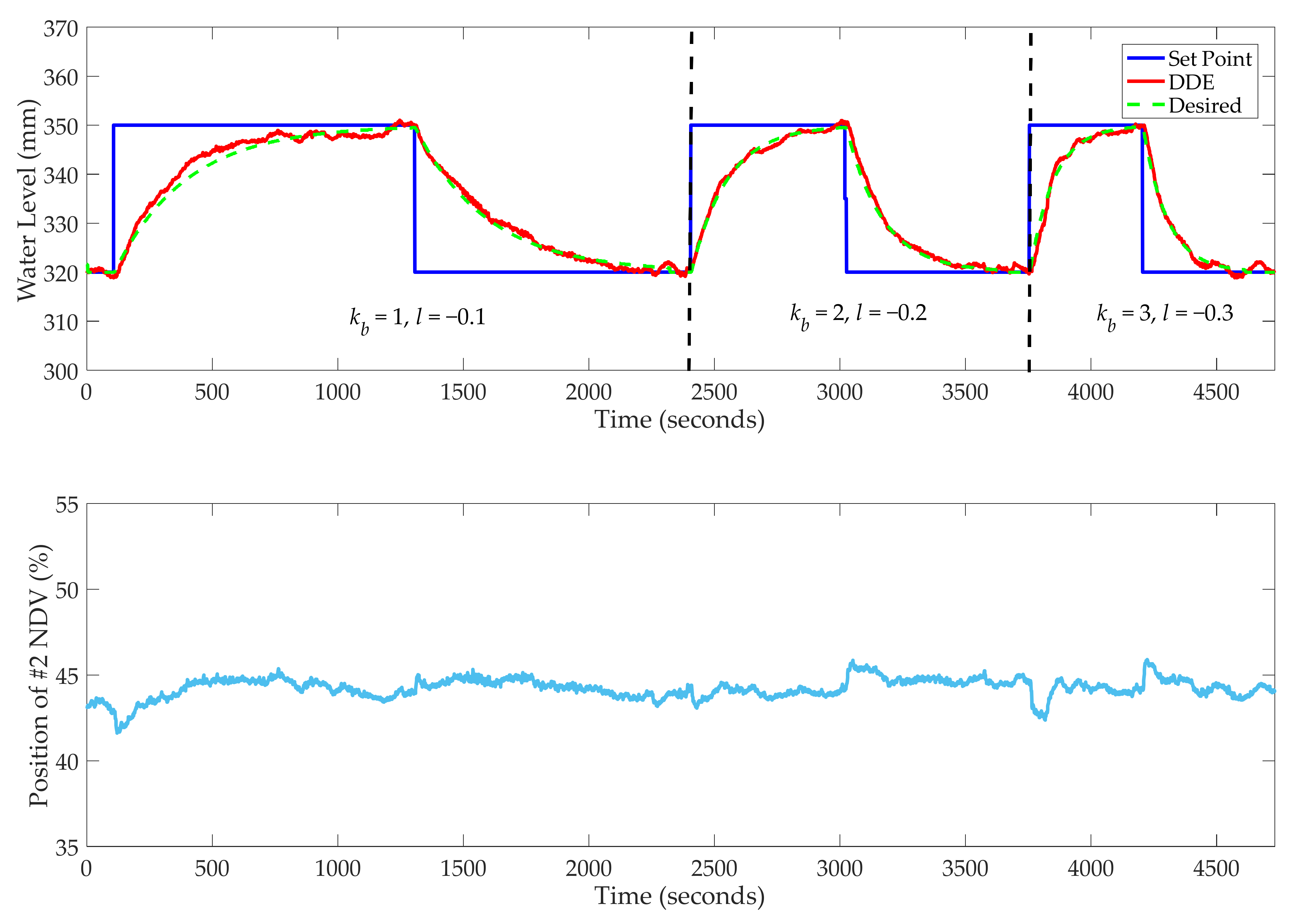
  • In terms of numerical simulations, kb can be augmented or reduced by 0.01 or 0.001; However, as for field tests on the coal-fired power plants, kb is recommended to be augmented by 1 and reduced by 0.1 due to the limited time;
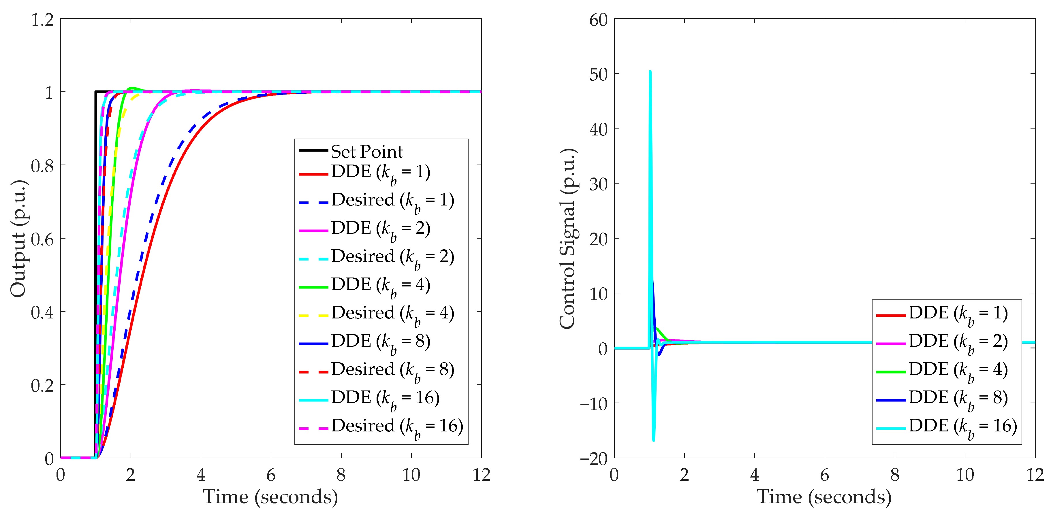
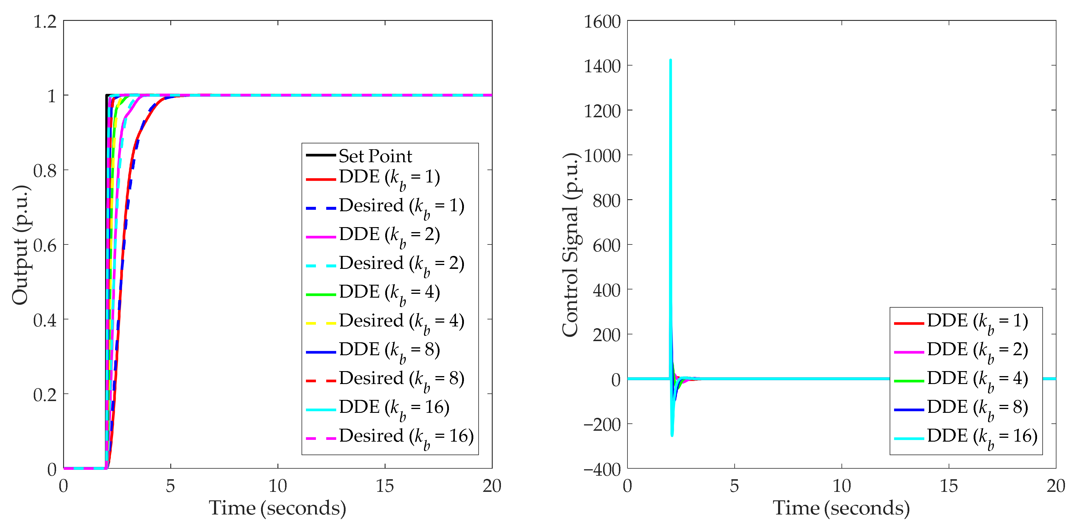
  • Using the proposed procedure, the limit of tracking the desired dynamic response is able to be found for the determined criteria;
  • Based on the proposed method, DDE PI or PID is tuned without using any specific plant model but the time scale of the process;
  • The systematic selection of the optimum set of PID parameters has therefore been categorized as a non-deterministic polynominal (NP) time-hard problem in terms of complexity [26,47]. Nevertheless, in terms of the proposed procedure, only one parameter, l, is being tuned monotonously for DDE PI or PID, which reduces the complexity of PID tuning.

5. Illustrative Examples

To demonstrate the effectiveness of the proposed desired dynamic selection procedure for DDE PI or PID, 10 typical systems were selected, as were the plants. Their transfer function models are able to describe most industrial processes. Table 1 lists the transfer function models of 10 typical systems.

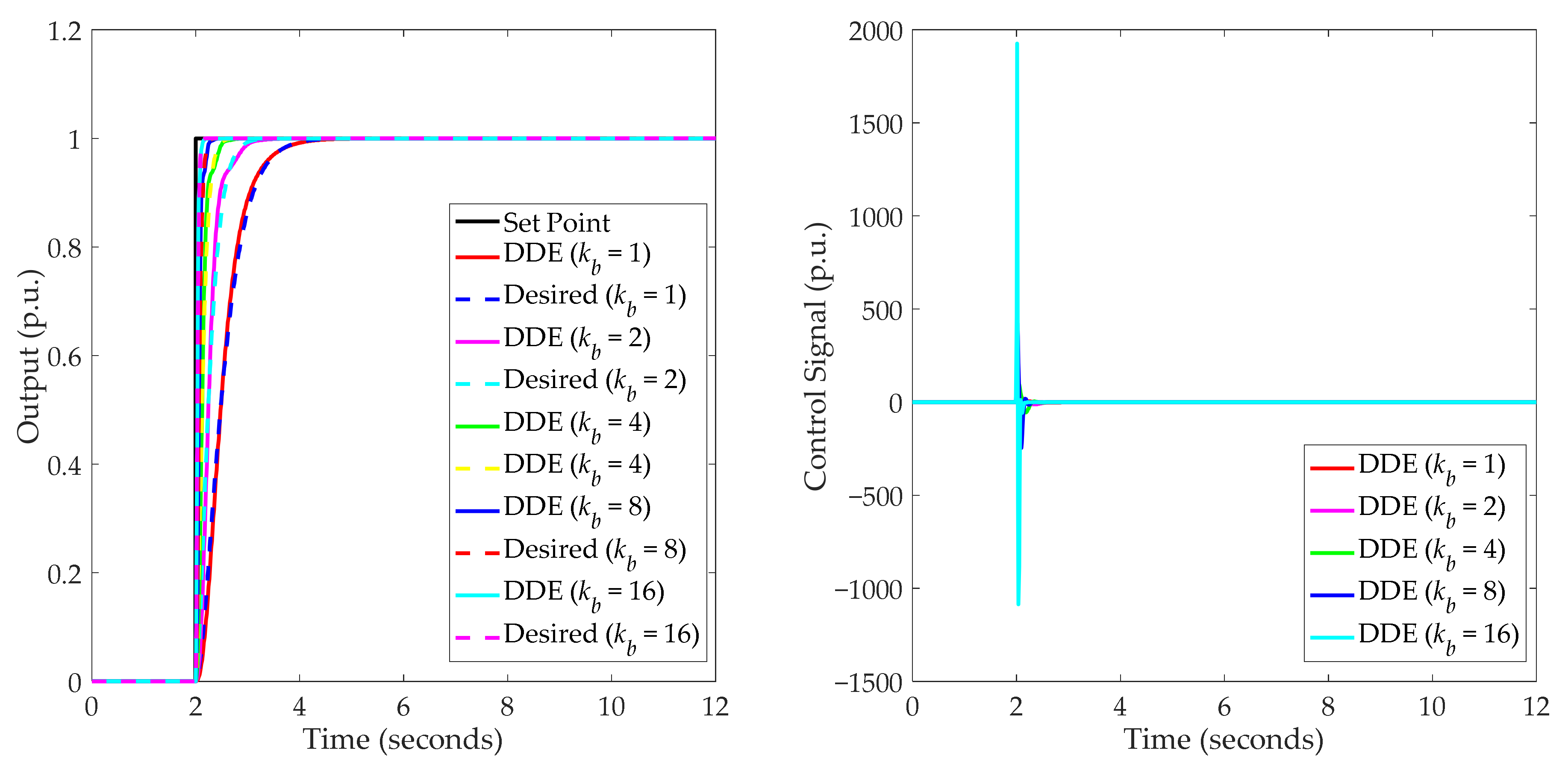
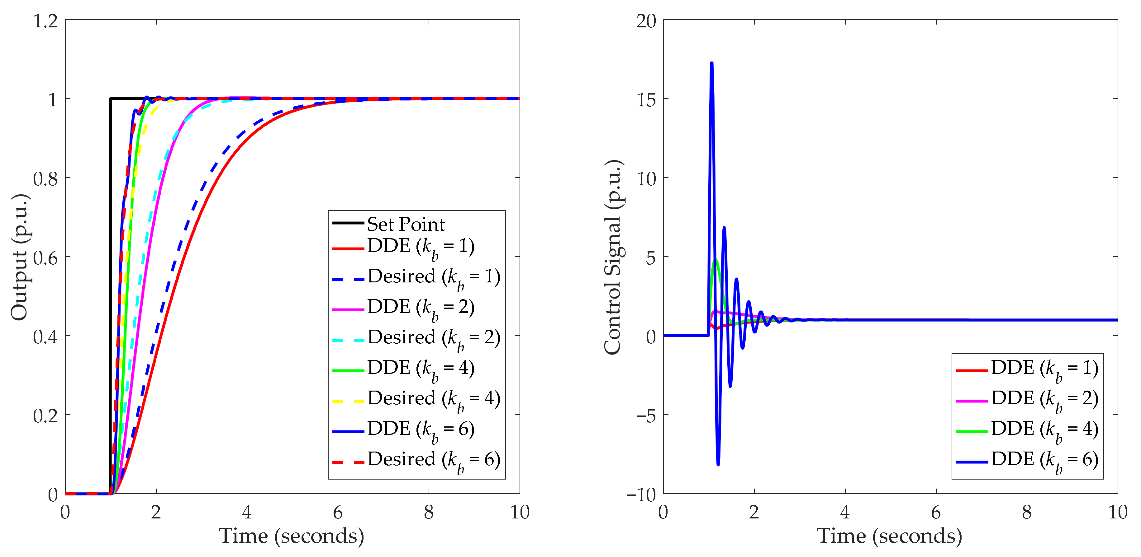
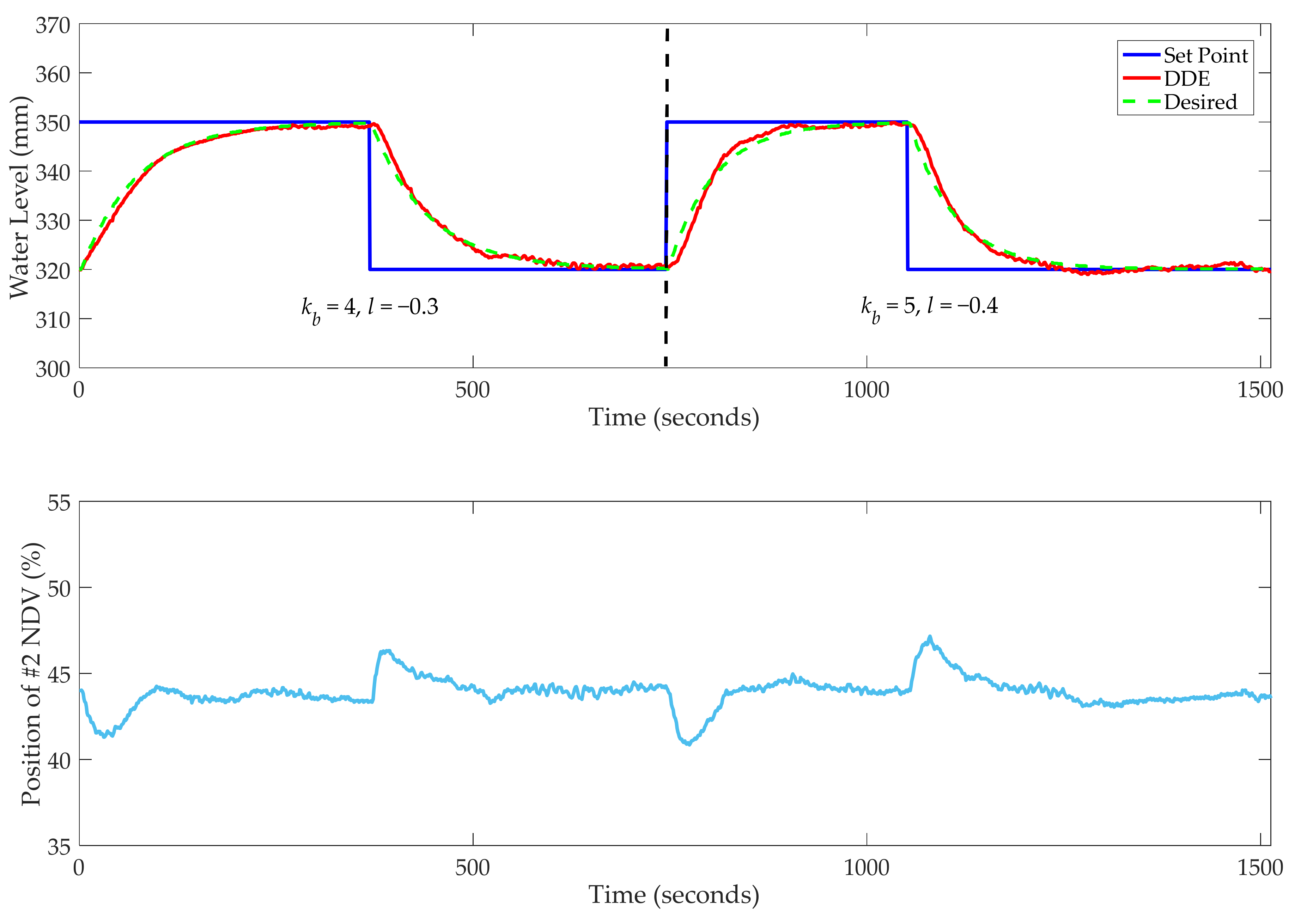
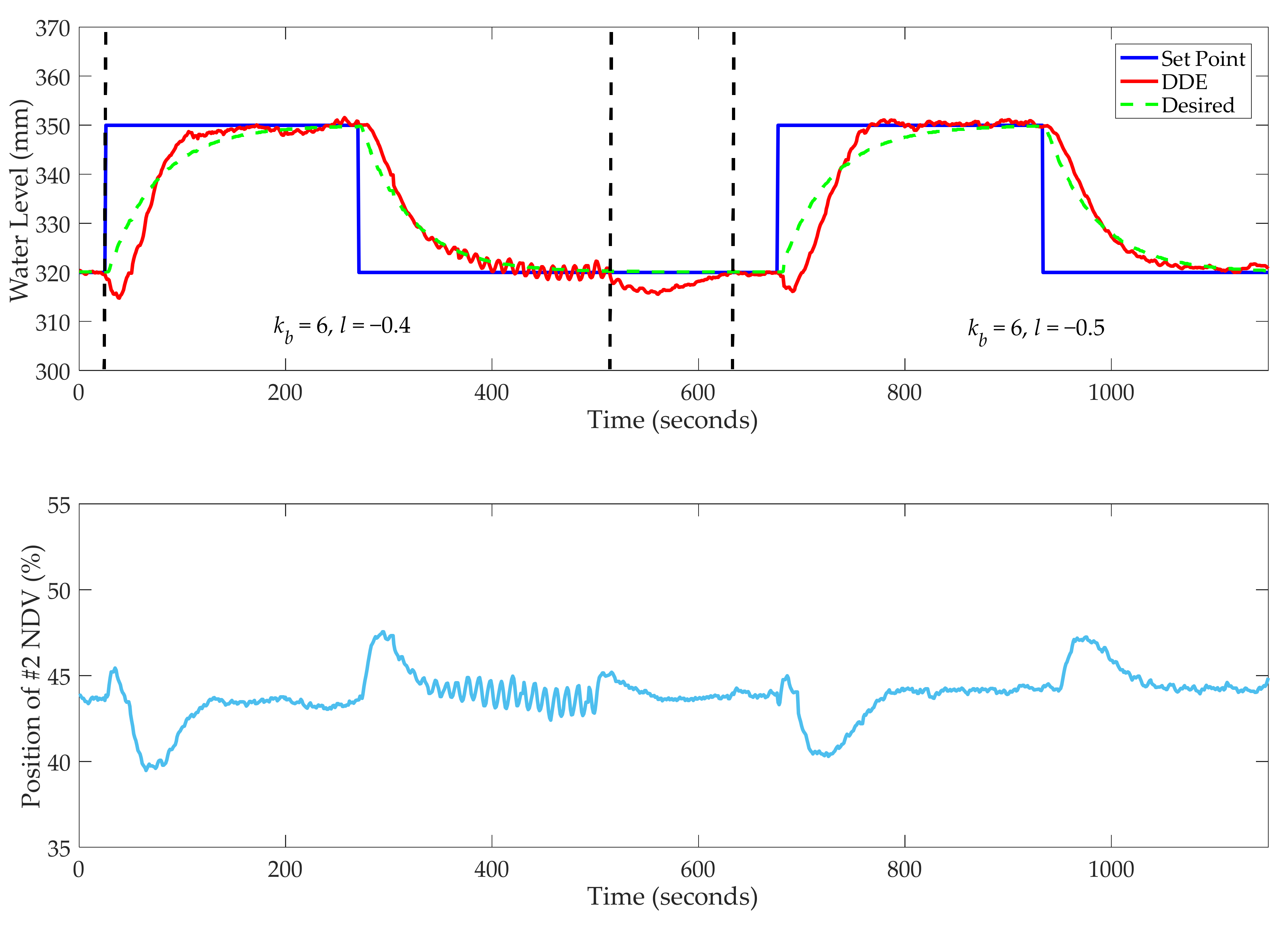
5.1. The Limit of Desired Dynamic Selection

It has been pointed out in [37] that the maximum uncertainty that can be dealt with by the feedback mechanism is described by a ball with a radius of 3 / 2 + 2 in a certain normed function space. Therefore, the unknown uncertainties, including internal (structure) uncertainty and external (disturbance) uncertainty, are unable to be handled by the feedback control system when their maximums are out of the ball.
Since DDE PI and PID are feedback control strategies, their ability to deal with uncertainties, also known as the total disturbance, is limited as well. If uncertainties are not dealt with by DDE PI or PID, the closed-loop output cannot possibly follow the characteristics of the desired dynamic equation. Consequently, the limit of the closed-loop desired bandwidth ωd exists. If ωd is selected beyond its limits, the closed-loop output of DDE PI and PID is unable to track the desired dynamic response accurately (i.e., all criteria in Section 4.2 are satisfied). In this subsection, the limit of the desired dynamic selection is discussed using numerical simulations.
First, for some plants, their limits on desired dynamic selection are mainly determined by the actuator and not the characteristics of the process. As a result, the desired dynamic response can be set almost as fast as the set point. Taking Gp1(s), Gp8(s) and Gp10(s) as examples, Figure 9, Figure 10 and Figure 11 show the performance of DDE PID with different desired dynamic responses for these processes.
From Figure 9, Figure 10 and Figure 11, it is obvious that the closed-loop output of DDE PID can track the desired dynamic response accurately even when kb is equal to 16. However, with the increase in kb, the variation of the control signal will be stronger, which may lead to actuator saturation. As a result, for these processes, their limits on ωd are mainly determined by the actuator.
Another aspect that should be addressed is that a transfer function model can describe the characteristics of several practical systems whose amplitude limits for the actuators are different. Therefore, in terms of illustrative examples, it is difficult to set the amplitude limits so that only constraints on the process are considered for numerical simulations. The constraints on the actuator are considered for experiments and field tests in this paper.
Second, for some plants, the desired dynamic selection of DDE PI and PID are mainly constrained by their characteristics. Taking Gp4(s), Gp7(s) and Gp9(s) as examples, Figure 12, Figure 13 and Figure 14 show the performance of DDE PID with different desired dynamic responses for these processes.
From Figure 12, Figure 13 and Figure 14, it is obvious that the limits of ωd for Gp4(s), Gp7(s) and Gp9(s) are determined by the characteristics of processes. Without the consideration of actuator saturation, in terms of Gp4(s), the limit of ωd exists between 4ωd0 and 6ωd0. As for Gp7(s), the limit of ωd exists between ωd0 and 2ωd0. In regard to Gp9(s), the limit of ωd exists between 0.1ωd0 and 0.2ωd0. Therefore, for these systems, their limits of ωd are determined by the characteristics of the processes.
Based on the selection procedure proposed in Section 4.3, and without the consideration of actuator saturations, the limits of ωd for 10 typical process are evaluated in Table 2. Note that kb is augmented or reduced by 0.1 in this section.
From Table 2, in terms of Gp1(s), Gp2(s), Gp8(s) and Gp10(s), their limits for ωd are unable to be evaluated without the consideration of actuator saturations. Aside from that, for other processes, their desired dynamic selections are constrained by their characteristics.
According to the results presented in Table 2, DDE PI and PID controllers designed based on the selection procedure are compared with several PID controllers tuned based on classical engineering tuning methods in the following subsection.

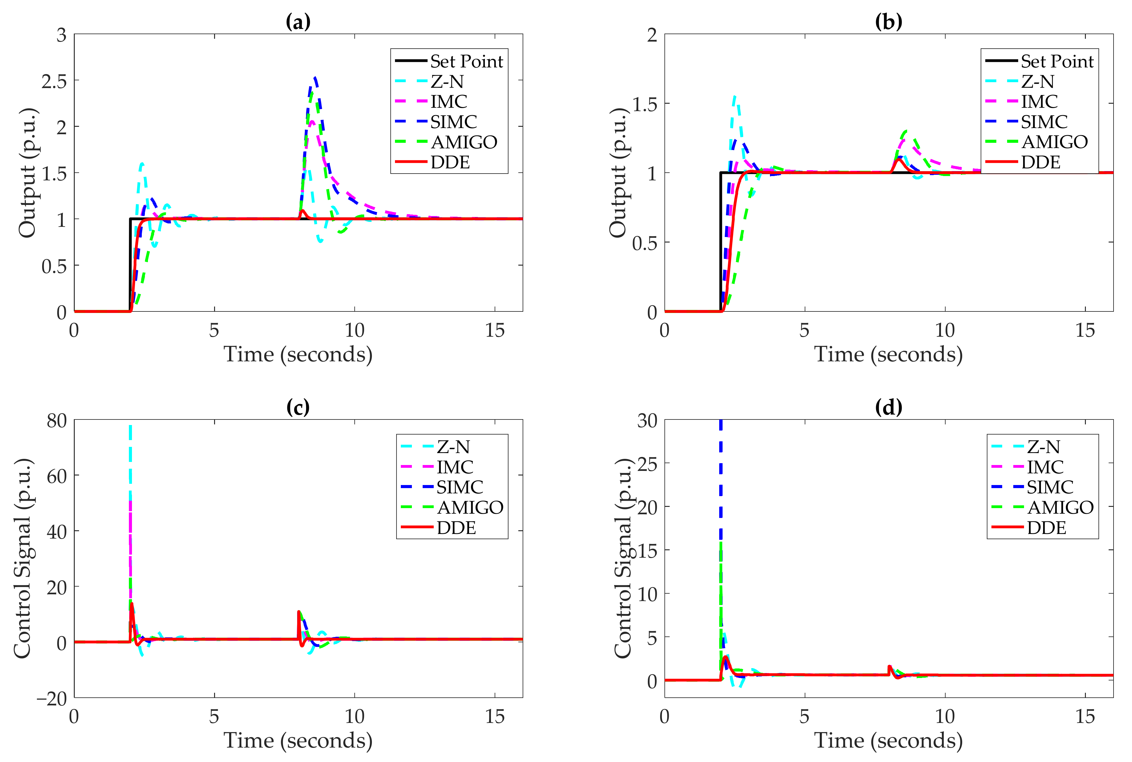
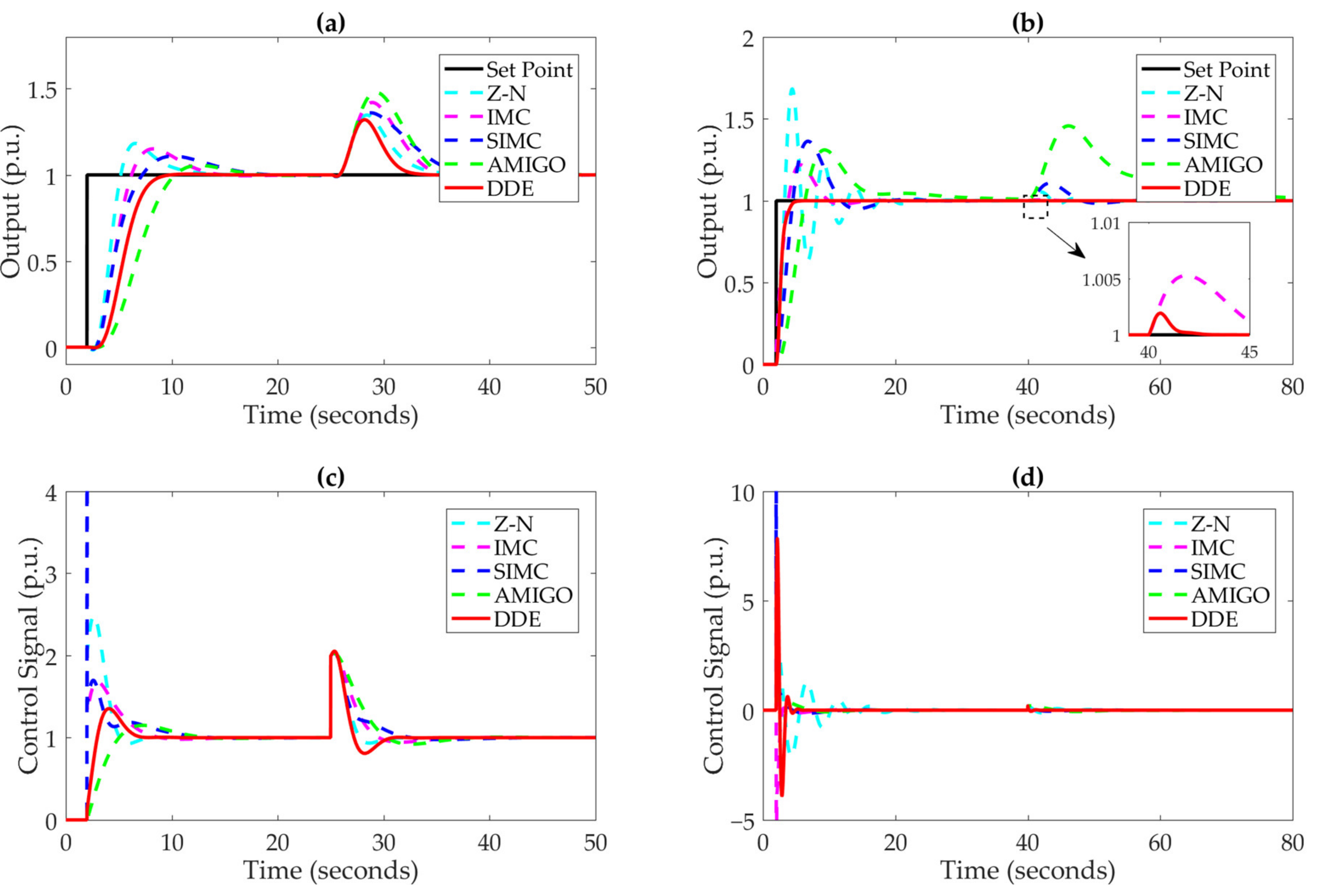
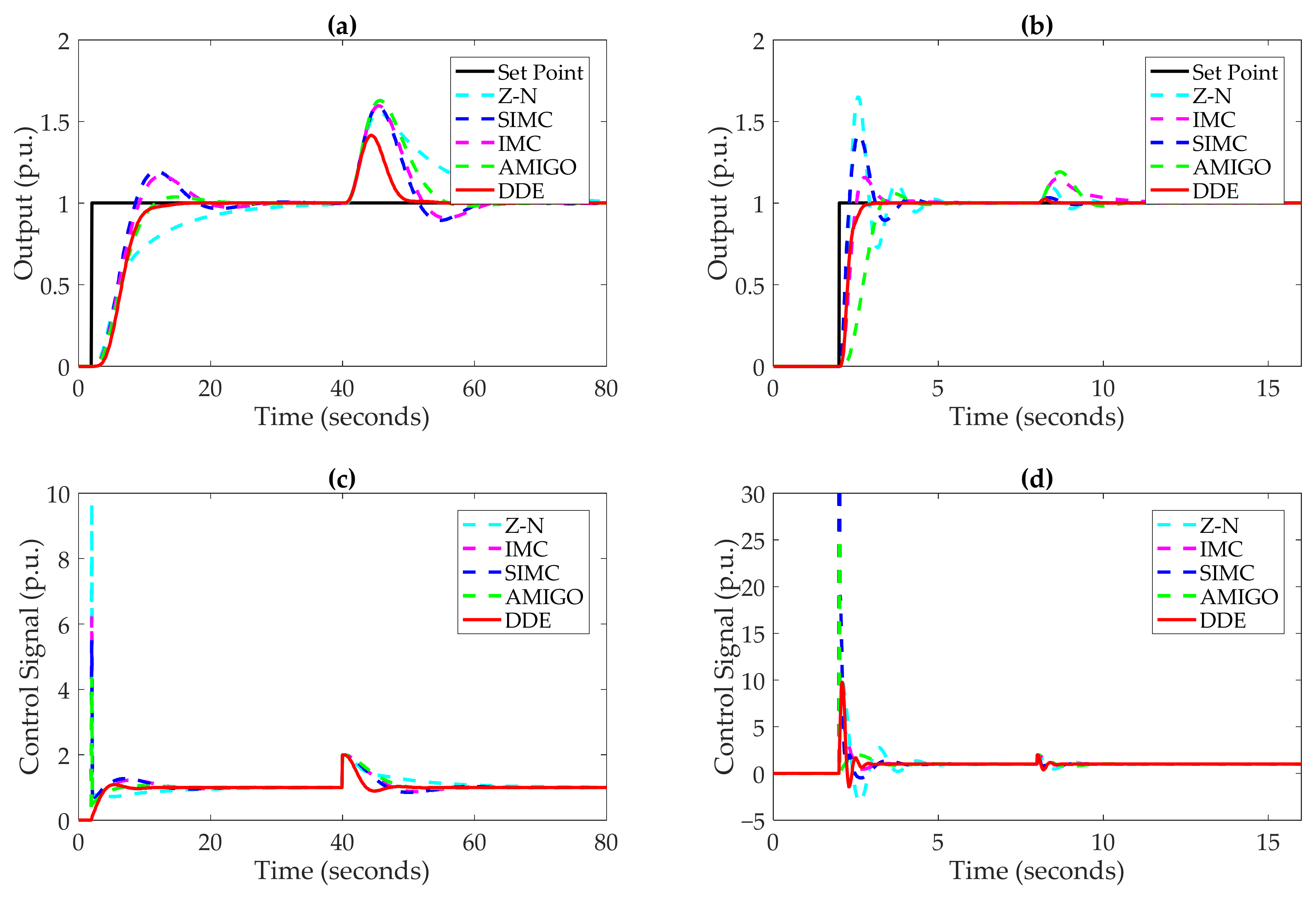
5.2. Comparisons with Practical PID Controllers

In this subsection, the proposed PID tuning method is compared with several classical tuning methods which are widely used by engineers, including the Z-N method [15], IMC method [16], SIMC method [17] and approximated MIGO (AMIGO) method [48]. Among them, AMIGO PI and PID have the structure illustrated in Figure 1. Table 3 lists the parameters of different PID controllers. Note that kb is selected to be no smaller than one for Gp1(s), Gp2(s), Gp8(s) and Gp10(s).
According to Table 3, it is obvious that the comparative tuning methods are not applicable for all processes since they are proposed based on specific transfer function models. However, the proposed method is available for these 10 typical processes because it only utilizes the time scale of the process. Based on the parameters listed in Table 3, Figure 15, Figure 16, Figure 17, Figure 18 and Figure 19 show the control performance of different PID controllers for 10 typical processes. Note that the set point has a unit step change, and step disturbances are added after the closed-loop output is stable.
From Figure 15, Figure 16, Figure 17, Figure 18 and Figure 19, the following comments can be summarized:
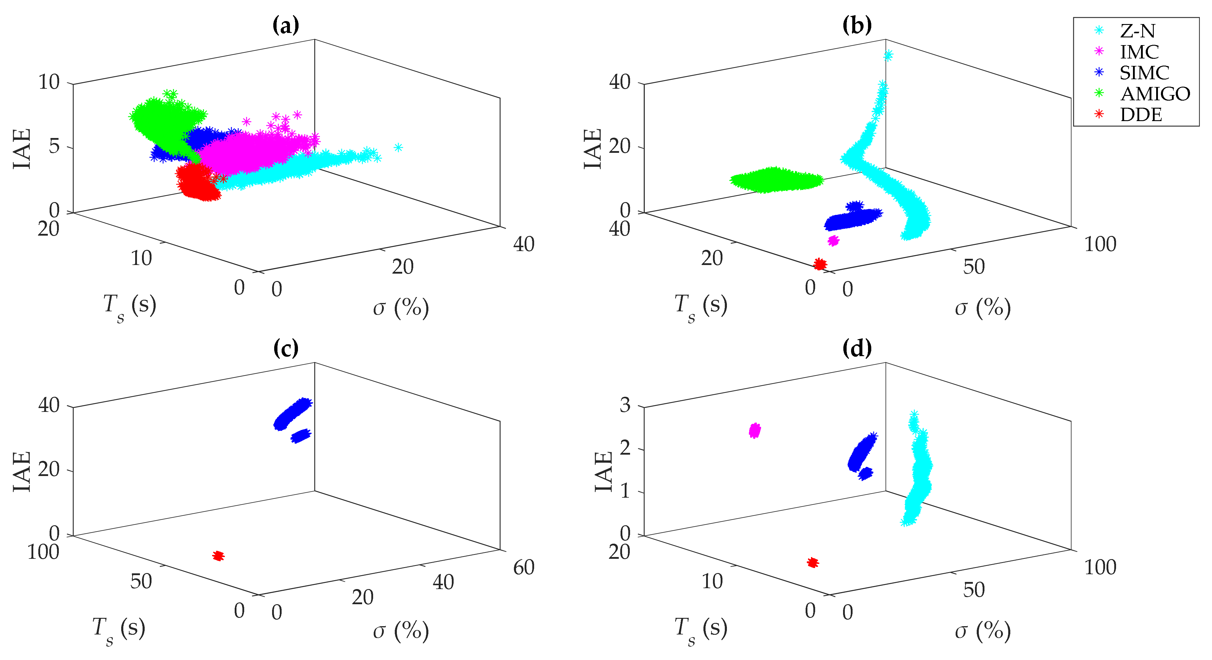
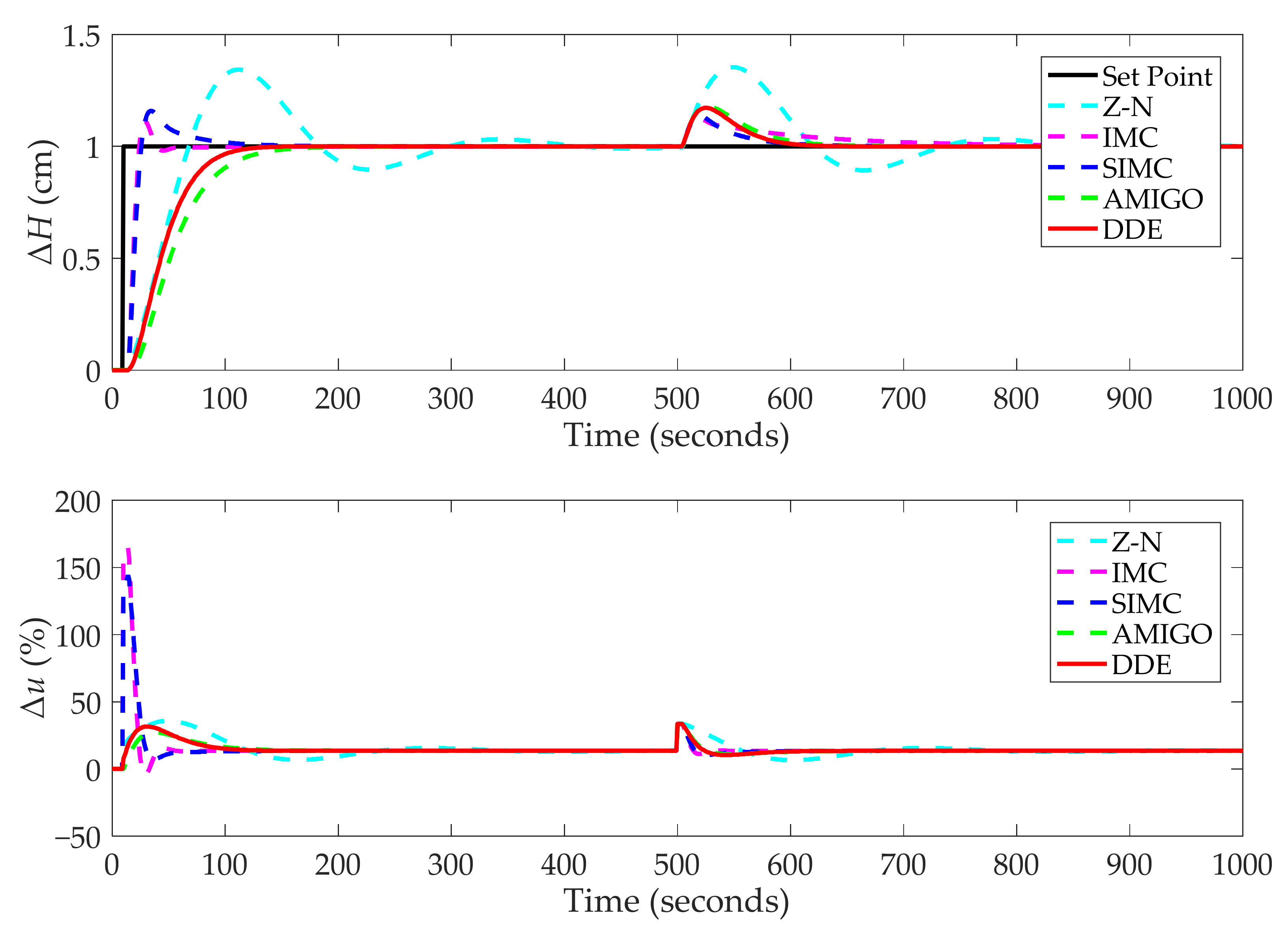
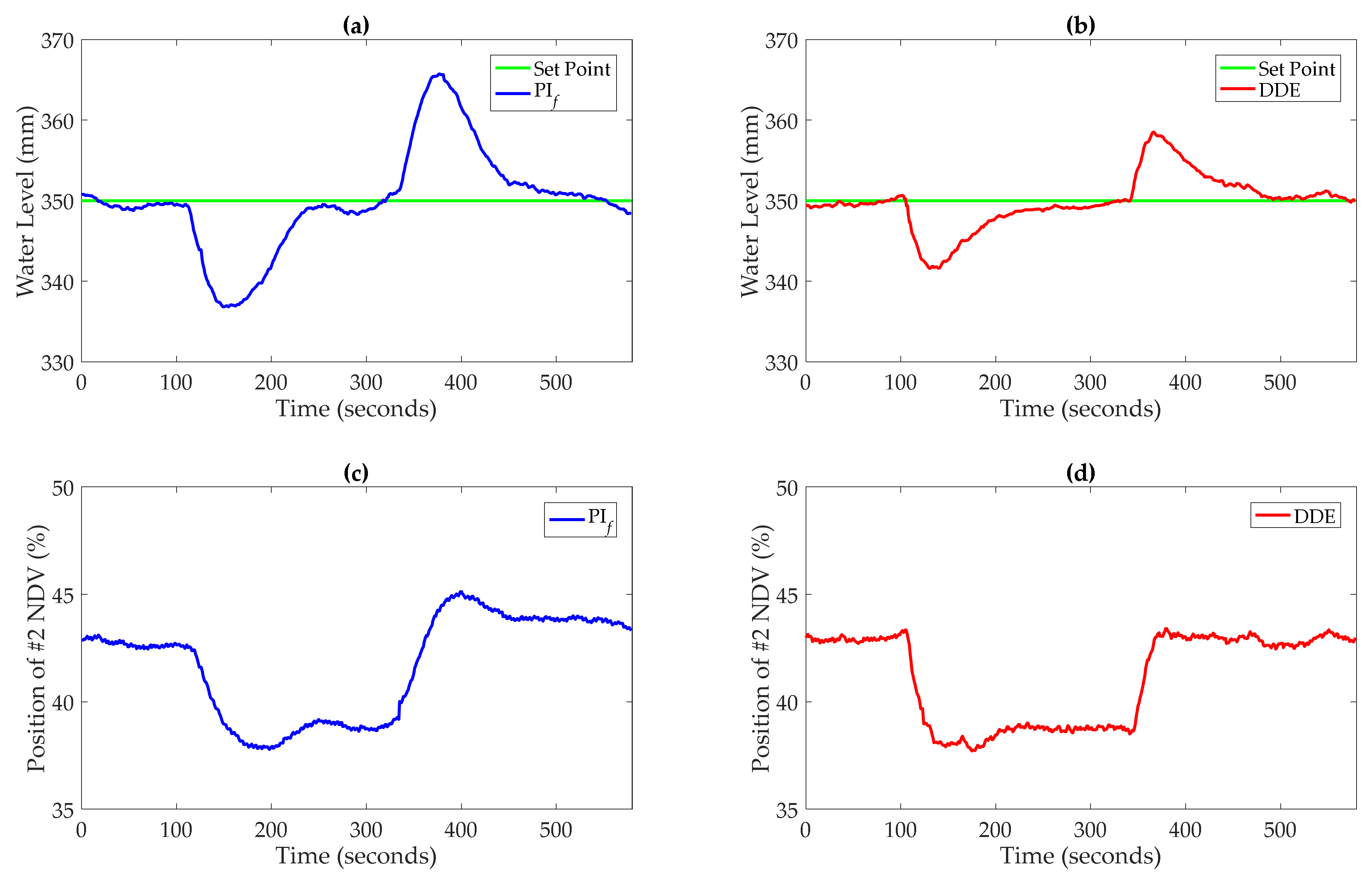
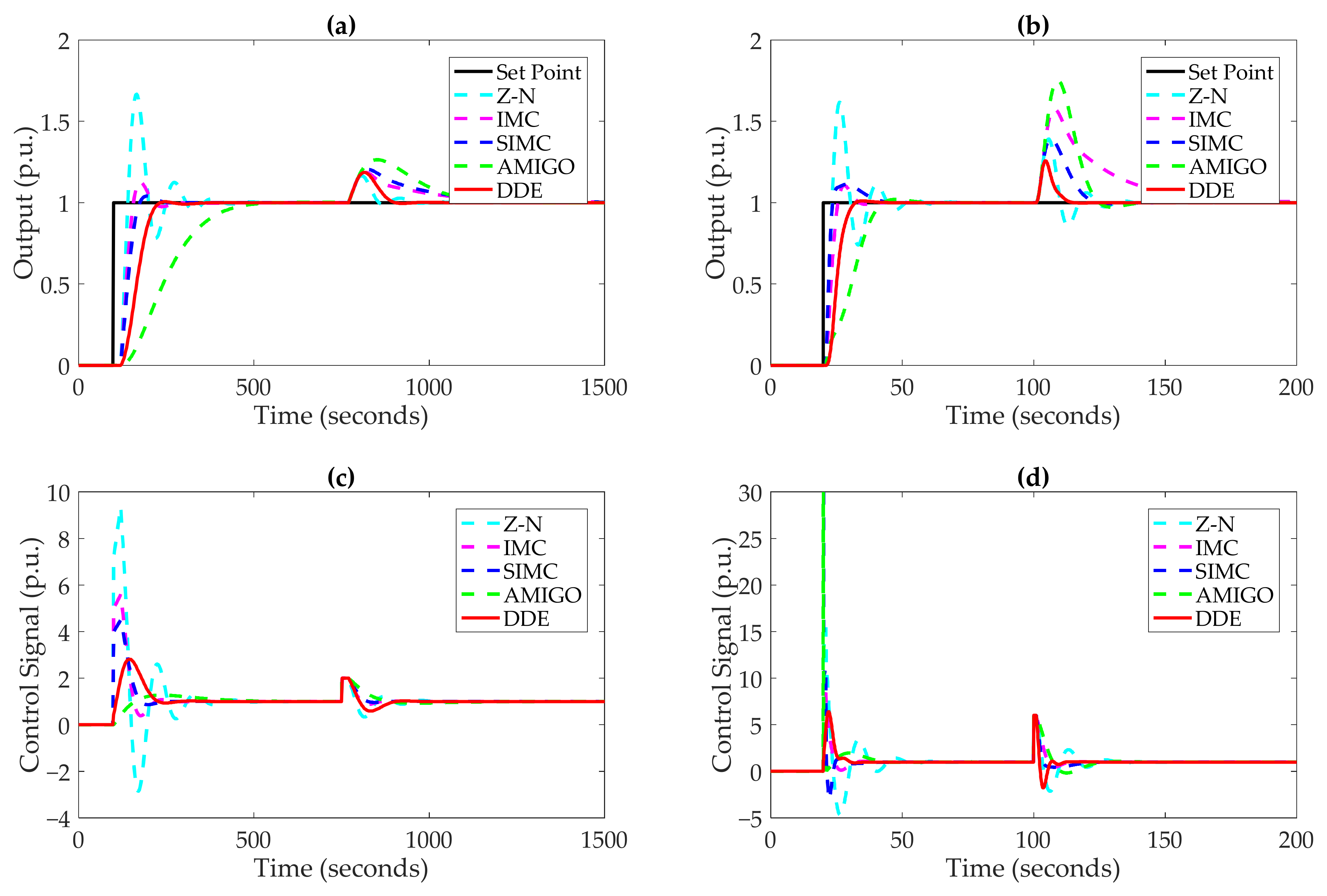
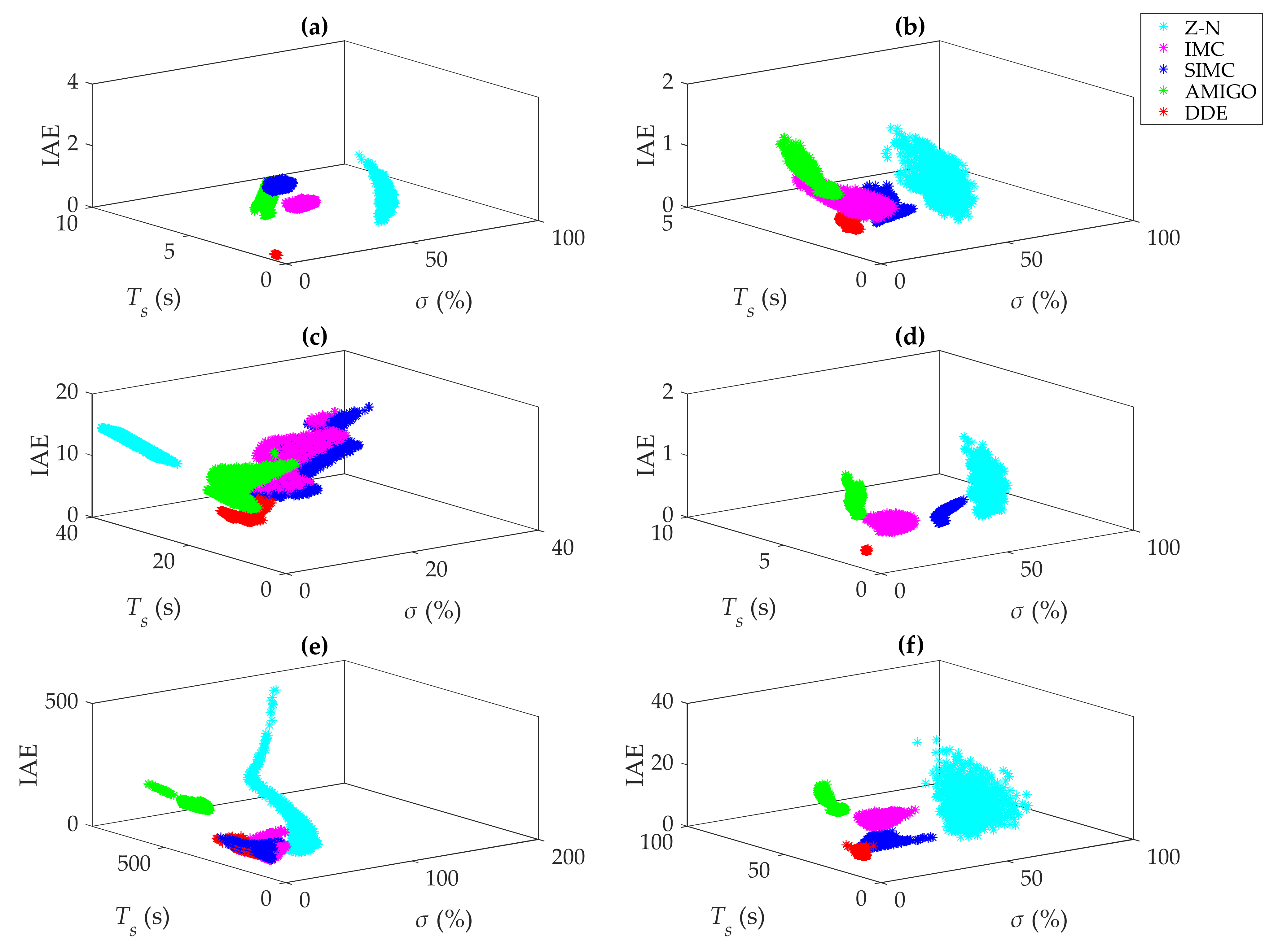
  • Compared with other PI and PID controllers, DDE PI and PID have moderate tracking performance and better disturbance rejection performance;
  • It is obvious that IMC PI and PID and SIMC PI and PID can obtain fast tracking performance with a small overshoot for Gp5(s) and Gp6(s) because they are proposed based on the nominal FOPDT and SOPDT systems. If the process model is mismatched, their reference tracking may exhibit significant oscillation;
  • The control performance of AMIGO PI and PID is conservative.
To quantitatively evaluate the control performance of different PI and PID controllers, dynamic indices, such as the overshoot (σ), the settling time (Ts) and the IAE of reference tracking (IAEsp) and disturbance rejection (IAEud), are calculated. The table of dynamic indices is presented in Appendix C due to the excess of figures.
In a practical industrial process, uncertainties may exist such that robustness is of significance to the controllers. Monte Carlo simulation is an effective method because it can intuitively demonstrate which controller has stronger robustness and better dynamic performance [49,50]. To test the robustness of different PI and PID controllers, the coefficients of the plant models of 10 typical processes were perturbed within a range of ±20% 1000 times. That aside, during the Monte Carlo trials, dynamic indices, such as σ, Ts and IAE (IAEsp + IAEud), were recorded. Figure 20 and Figure 21 illustrate the results of 1000 Monte Carlo trails of different PI and PID controllers.
More intensive scatters mean stronger robustness. Moreover, if the scatters are closer to zero, the controller has better control performance. From Figure 20 and Figure 21, compared with other PI and PID controllers, DDE PI and PID can obtain stronger robustness and better dynamic performance, which shows their superiorities in reference tracking, disturbance rejection and handling uncertainties.

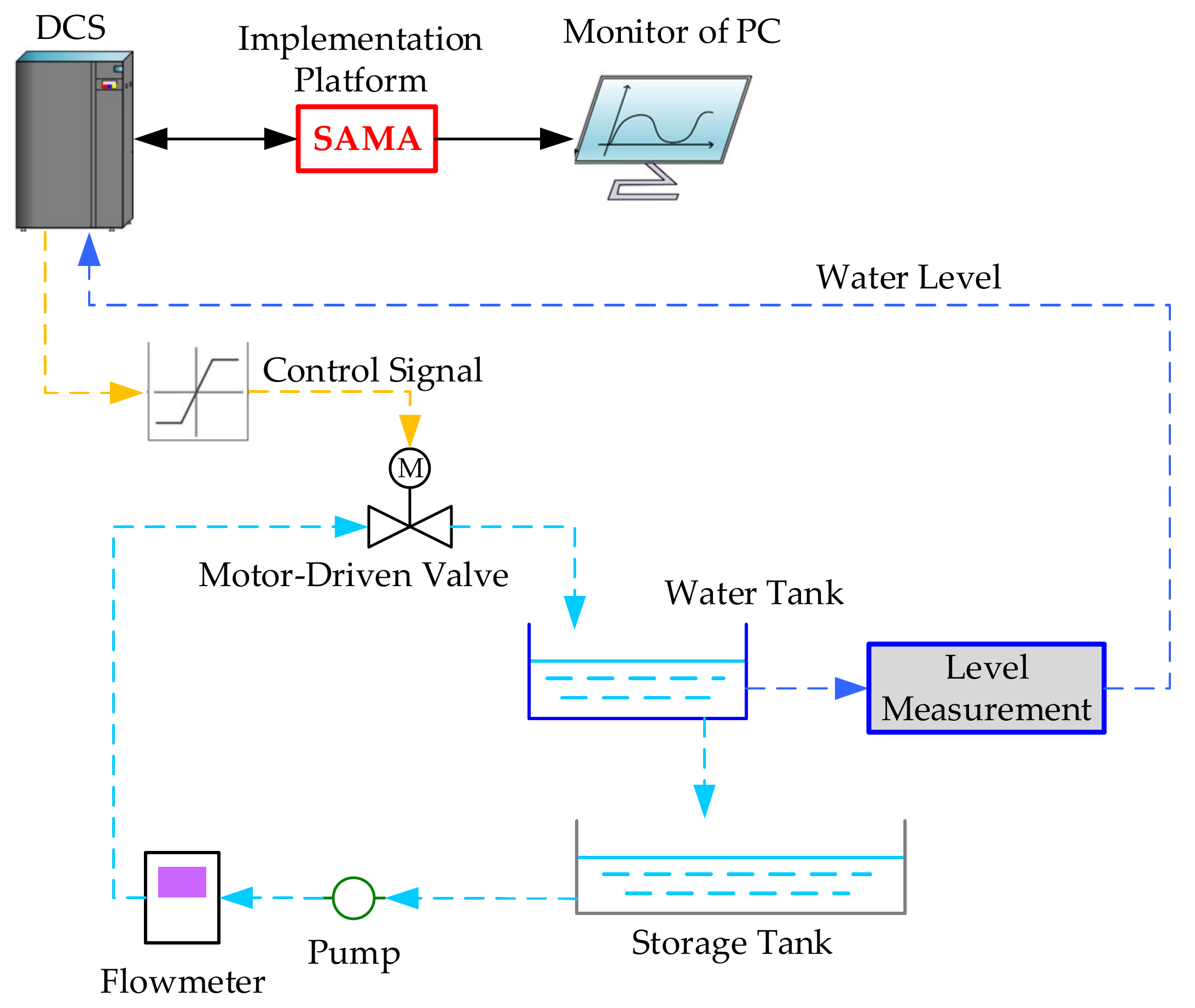
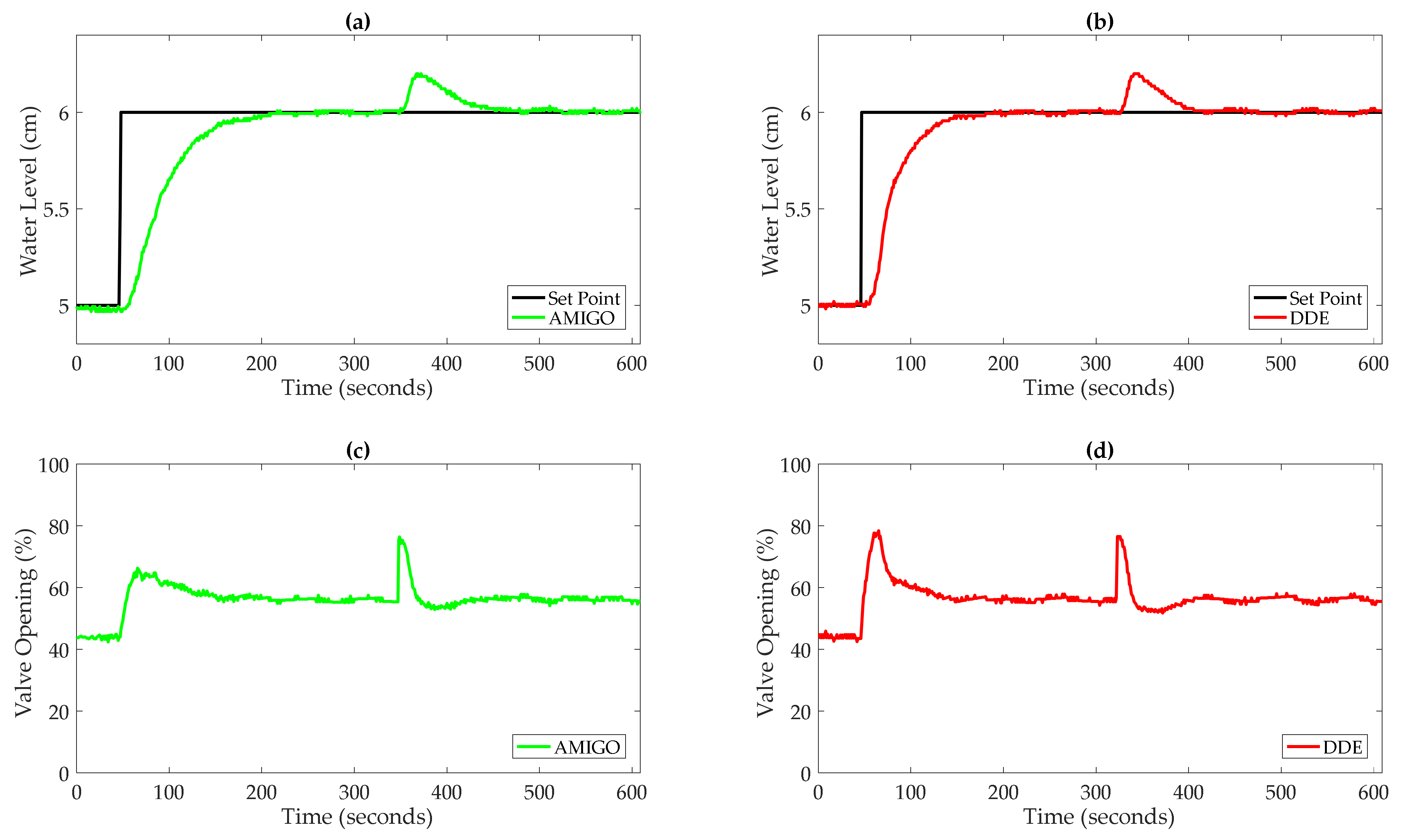
6. Experimental Verification with a Water Tank

Prior to industrial application, a laboratory experiment is necessary to confirm the feasibility of the proposed method, the validity of the theoretic analysis and the simulations above [51]. In addition, as for practical systems, PID controllers are rarely used for the reason that the derivative action may lead to self-oscillations of the control signal when measurement noise exists [29]. As a result, in this section, a DDE PI controller designed based on the proposed selection procedure is applied to the level system of a water tank. In particular, all comparative controllers are designed based on PI controllers as well.

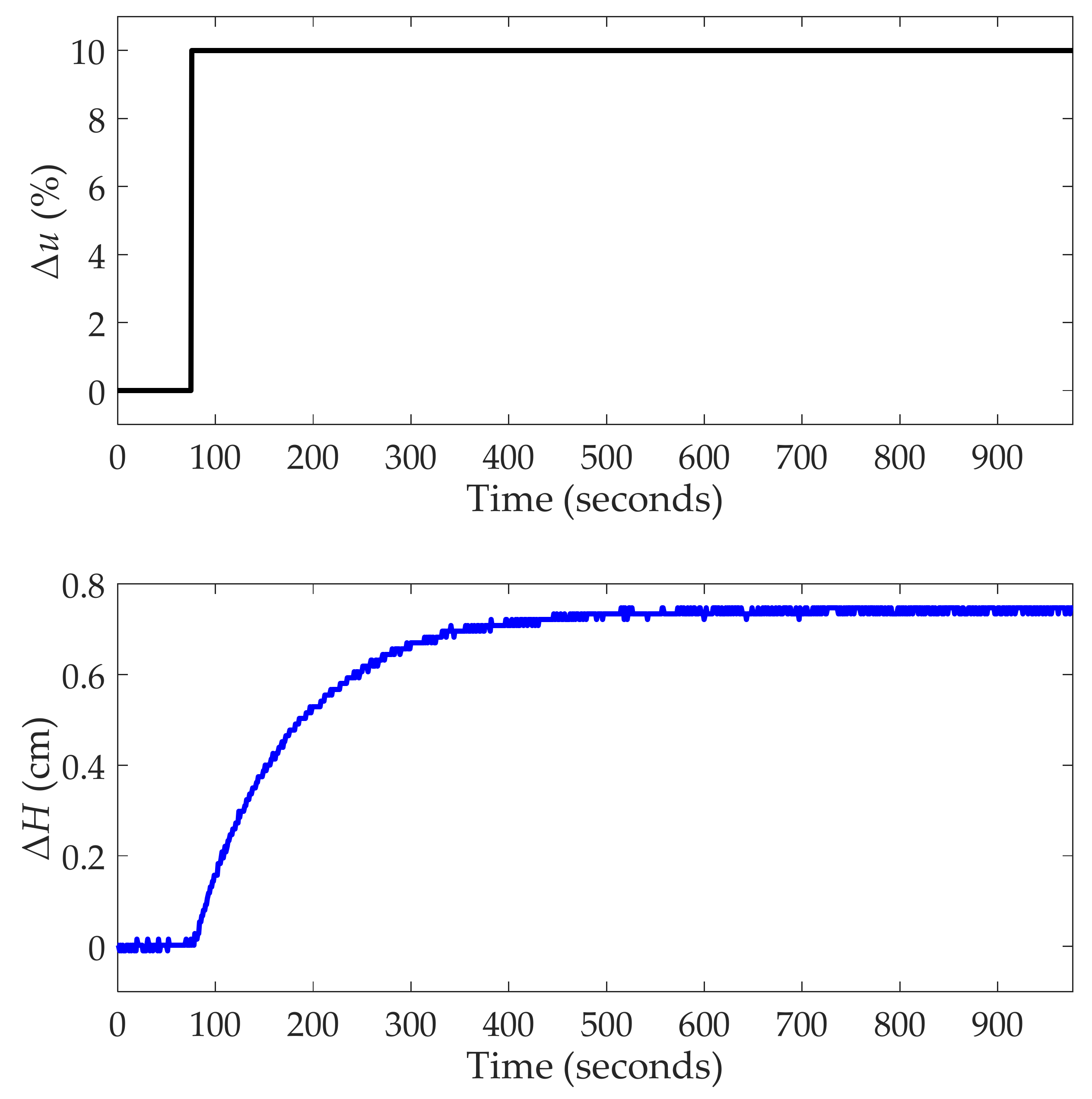
6.1. Experimental Set-Up and Process Description

Figure 22 shows the schematic structure of the experimental set-up, which mainly contains the water tank, the storage tank, the motor-driven valve, the pump, the flowmeter and the DCS. All controllers were implemented on the DCS, whose sample time was 1 s.
To calculate the initial parameters of DDE PI, an open-loop test was carried out. During the test, the opening of the motor-driven valve had a step change with an amplitude of 10% at 75 s. Figure 23 illustrates the results of the open-loop test.
In Figure 23, Δu and ΔH are denoted as changes in the valve opening and the water level, respectively. According to the results, the time delay τ and the response time tp of the process were evaluated to be 5 s and 384 s, respectively. Aside from that, the gain in the process was calculated to be 0.074. Therefore, the initial parameters of DDE PI could be evaluated as ωd0 = 0.0103, k0 = 0.103 and l0 = 0.0076.

6.2. Results and Discussions

First, DDE PI was designed based on the desired dynamic selection procedure summarized in Section 4.3. Since the water tank is a nonlinear system in practice, the controller will obtain different performance when the set point has a positive step change and a negative step change. Therefore, the closed-loop output of DDE PI should satisfy all criteria in Section 4.2 when the level set point increases and decreases.
During the experiments, the parameter kb was augmented from 1 by a step of 1 and l was reduced from 0.007 by a step of 0.001. Figure 24 shows the experimental results of the DDE PIs when kb = 1, 2 and 3. Note that the level set point was varying between 5 cm and 6 cm.
From Figure 24, it is obvious that the closed-loop output of DDE PI could track the desired dynamic response accurately with almost no overshoot when l was tuned appropriately. Moreover, obvious oscillation and actuator saturation were nonexistent. To quantitatively evaluate whether all criteria were satisfied, the dynamic indices of DDE PIs with kb = 1, 2 and 3 are presented in Table 4.
According to Table 4, it is easy to learn that the overshoots and IAE errors of DDE PIs with kb = 1, 2 and 3 satisfied Criterion 1 and Criterion 2, respectively. Hence the closed-loop output of DDE PI could track the desired dynamic response accurately when kb = 1, 2 and 3.
However, when kb was augmented to four, the results for DDE PI changed. Figure 25 illustrates the experimental results for DDE PI with kb = 4.
As can be seen from Figure 25, obviously, the overshoot of the DDE PI was significant when the set point varied from 6 cm to 5 cm. Moreover, if l was reduced to 0.005, oscillation occurred when the set point increased from 5 cm to 6 cm. As a result, it would be more severe if l was smaller than 0.005, and the valve opening may have reached its upper limit. Table 5 lists the experimental dynamic indices of DDE PIs with kb = 4 in order to evaluate whether the closed-loop output could track the desired dynamic response accurately.
Based on Table 5, evidently, the overshoots and IAE errors were larger than 1% and 10%, respectively. Therefore, the limit of ωd existed between 3ωd0 and 4ωd0.
Second, comparative controllers were applied to the level control system of the water tank. Their designs were based on an identified FOPDT model of the process, which is depicted as 0.074 e 5 s 97 s   +   1 . Table 6 presents the parameters of different PI controllers.
Based on the parameters listed in Table 6, Figure 26 shows the simulation results of different PI controllers using the identified transfer function model. Note that the set point had a unit change at 10 s, and a step disturbance with an amplitude of 20 was added at 500 s.
As can be seen from Figure 26, there is no doubt that IMC PI and SIMC PI can obtain better control performance than the other controllers, especially regarding the reference tracking. In terms of the variations of the control signal, the peak values of IMC PI and SIMC PI were 164.5% and 144.2% if the set point varied with an amplitude of 1 cm, respectively. However, the opening of the motor-driven valve could only vary between 0% and 100%. As a result, IMC PI and SIMC PI may lead to severe actuator saturations when the level set point changes from 5 cm to 6 cm. That aside, compared with Z-N PI and AMIGO PI, DDE PI has advantages in both reference tracking and disturbance rejection.
Figure 27 and Figure 28 illustrate the control performance of Z-N PI, SIMC PI, AMIGO PI and DDE PI. Note that the set point had a step change from 5 cm to 6 cm, and a step disturbance for the valve opening with an amplitude of 20% was added after the water level was stable.
Based on Figure 27 and Figure 28, the following comments can be summarized:
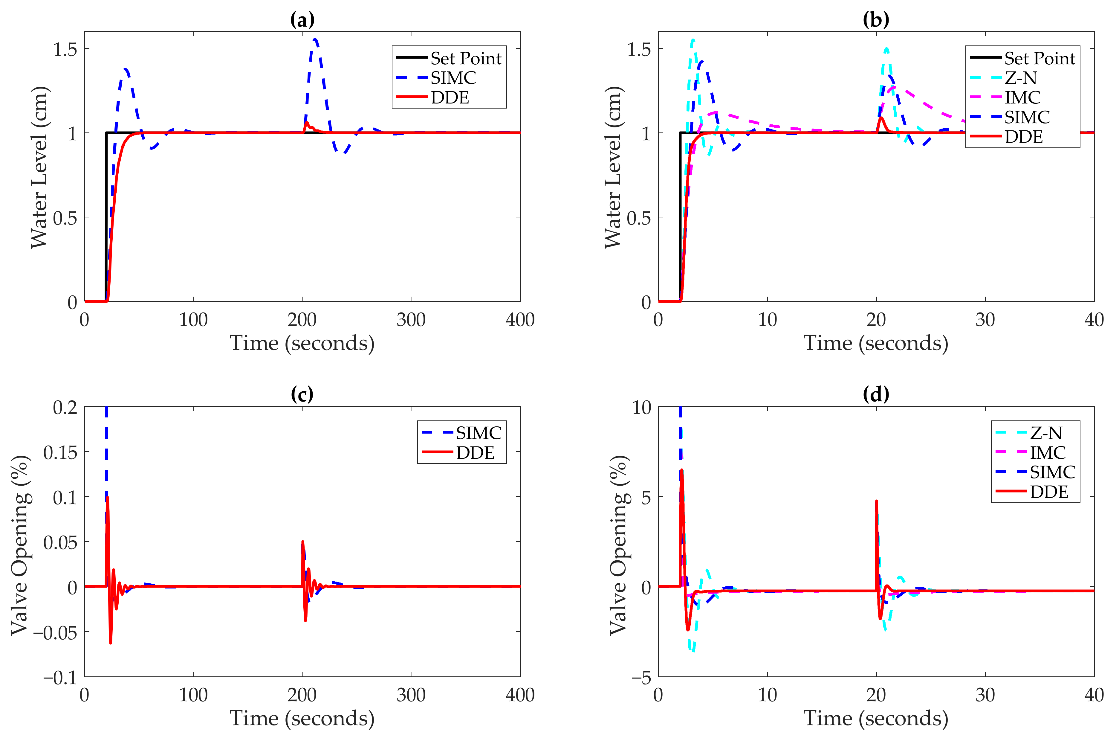
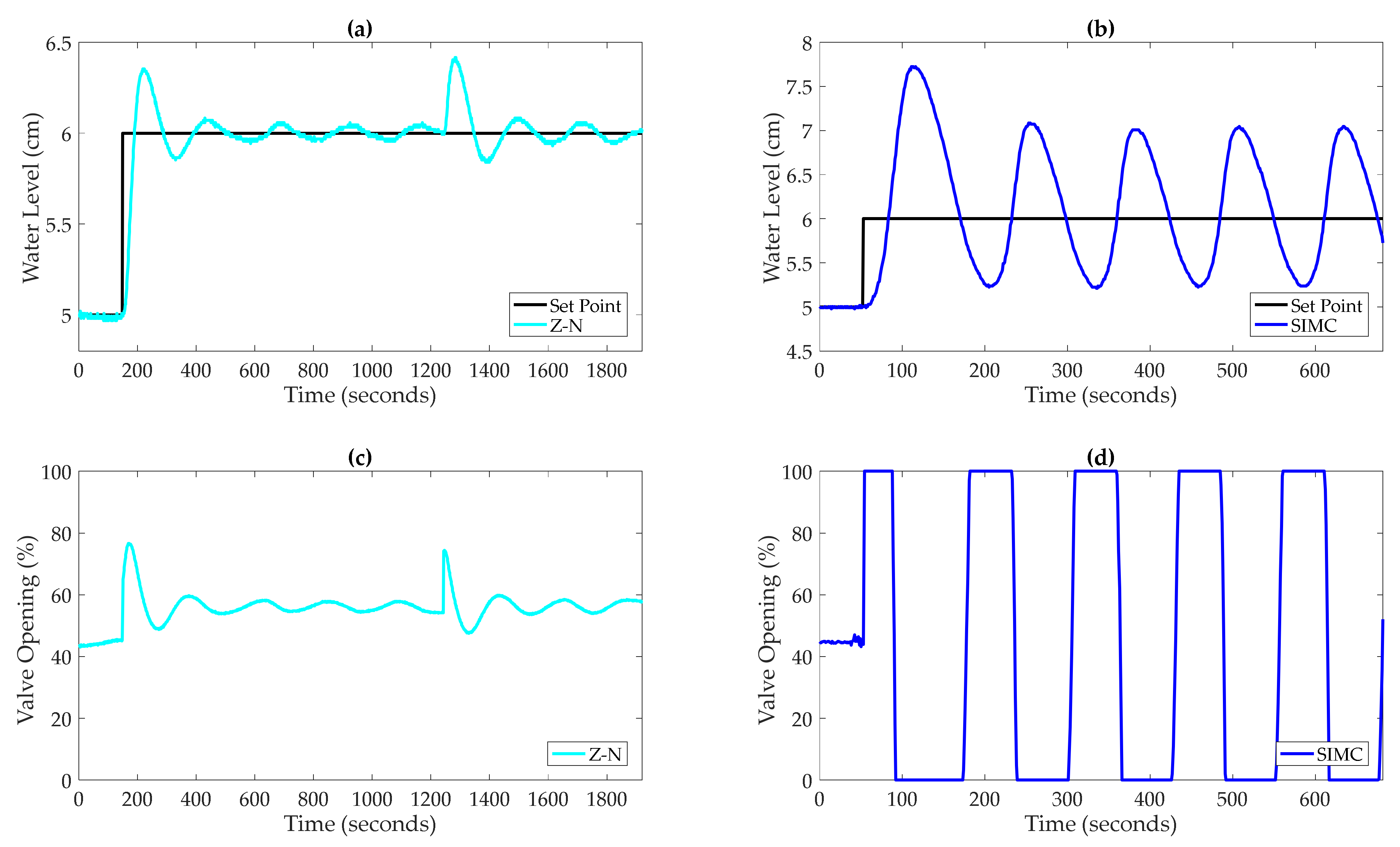
  • Compared with AMIGO PI, DDE PI had faster reference tracking performance;
  • Using the Z-N method, the water level may oscillate severely if the set point has a step change;
  • As expected, the application of SIMC PI would lead to actuator saturations, and the water level was unable to be stable.
  • From Table 6, IMC PI had stronger controller parameters than SIMC PI, which means that its variation in the valve opening was larger than that of SIMC PI. As a result, it was not applied to the level control of the water tank to protect the actuator.
To quantitatively evaluate the experimental results of different PI controllers, Table 7 lists the dynamic indices. Note that emax is denoted as the maximum deviation caused by the disturbance.
According to Table 7, DDE PI can obtain the smallest overshoot, shortest settling time and lowest deviation compared with other PI controllers. Therefore, the experimental results demonstrate the effectiveness of the proposed method in both reference tracking and disturbance rejection.

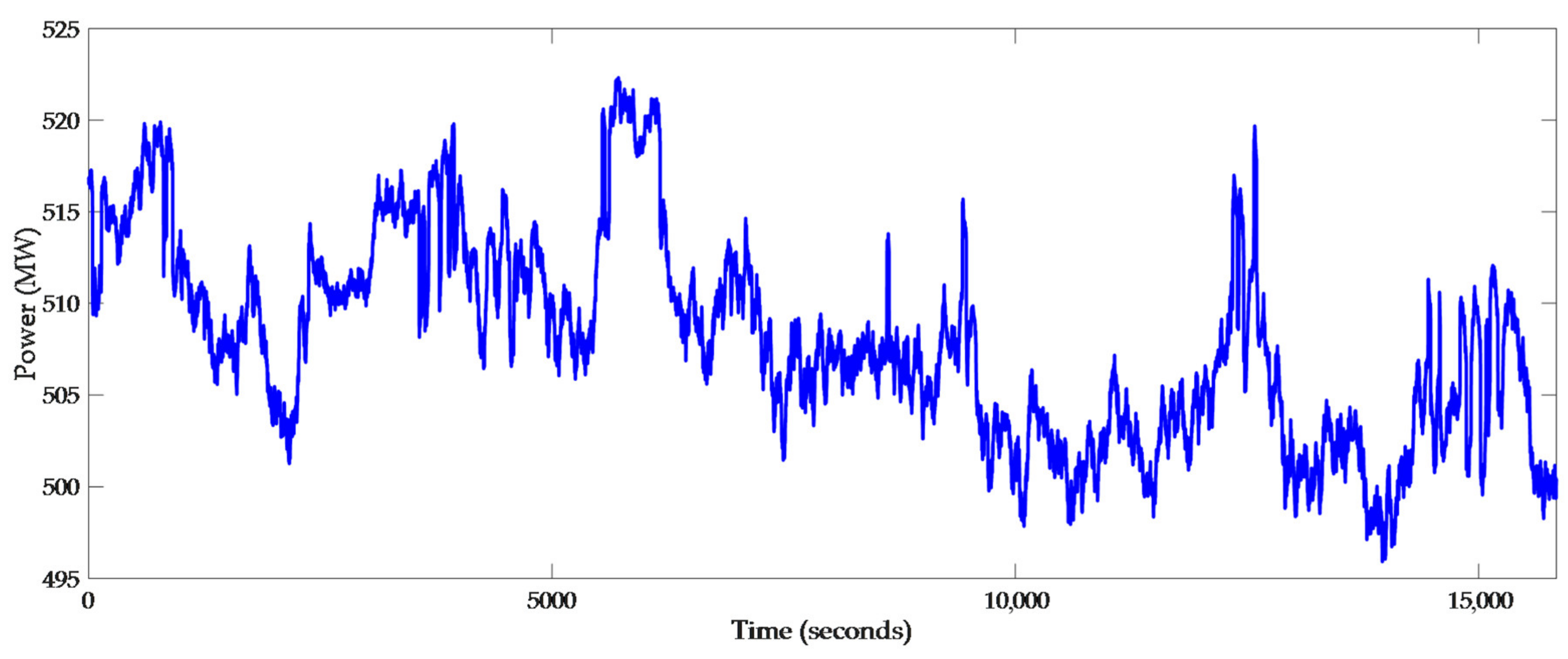
7. Field Test on an HP Heater of a 600-MW Coal-Fired Power Plant

Motivated by the encouraging results of the numerical simulations and laboratory experiments, a field test on a practical coal-fired power plant was carried out as described in this section based on DDE PI.

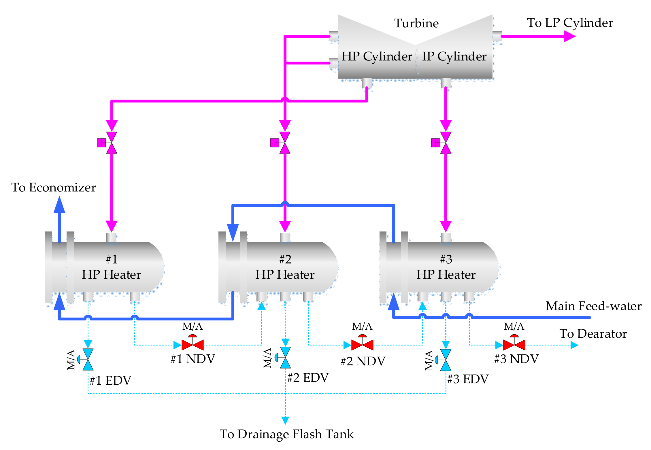
7.1. Process Description of the HP Heater

DDE PI was applied to the HP heater of an HP steam extraction and drainage system in a 600-MW in-service supercritical unit of a coal-fired power plant in Chaoyang, Liaoning Province, China, whose structure is illustrated in Figure 29. The HP heater is of importance to the feedwater regenerative system of the power plant. It is used to heat the boiler feedwater with high-temperature steam, which is extracted from the turbine [52].
The levels of the HP heaters are related to the efficiency of the daily operation of a unit. A higher or lower level than the set point may deteriorate the thermal economy or even threaten the safety of the unit [53]. Therefore, the level of the HP heater must be controlled at its desired value.
According to Figure 29, the level of HP heater #2 was more difficult to control for the reason that it was influenced by the levels of both HP heaters #1 and #3. As a result, tuned by the proposed selection procedure, DDE PI was designed to control the level of HP heater #2 in order to demonstrate its superiorities.
In terms of the process, the position of NDV #2 and the level of HP heater #2 were the manipulated variable and the controlled variable, respectively. Aside from that, disturbances were mainly caused by the position of EDV #2, the working fluid flux from HP heater #1 and the steam flux from the HP cylinder. Compared with other disturbances, the position of EDV #2 had a more significant impact on the level. The control goals of the HP heater are summarized as follows:
  • The primary goal was to regulate the level of the HP heater as close to its set point as possible in the face of various disturbances;
  • When the unit was starting or stopping, the fast reference tracking performance of the controller was required.
To evaluate the time scale of the process and obtain the initial parameters of DDE PI, an open-loop test was carried out when the load varied around 300 MW. Note that the position of NDV #2 had a step change with an amplitude of 2%. Figure 30 shows the results of the open-loop step test.
According to the results, the time delay τ and the response time tp of the process were evaluated to be 3 s and 1125 s, respectively. Additionally, the gain of the process was calculated to be 59.5. Therefore, the initial parameters of DDE PI could be evaluated as ωd0 = 0.0035, k0 = 0.035 and l0 = −1.32.

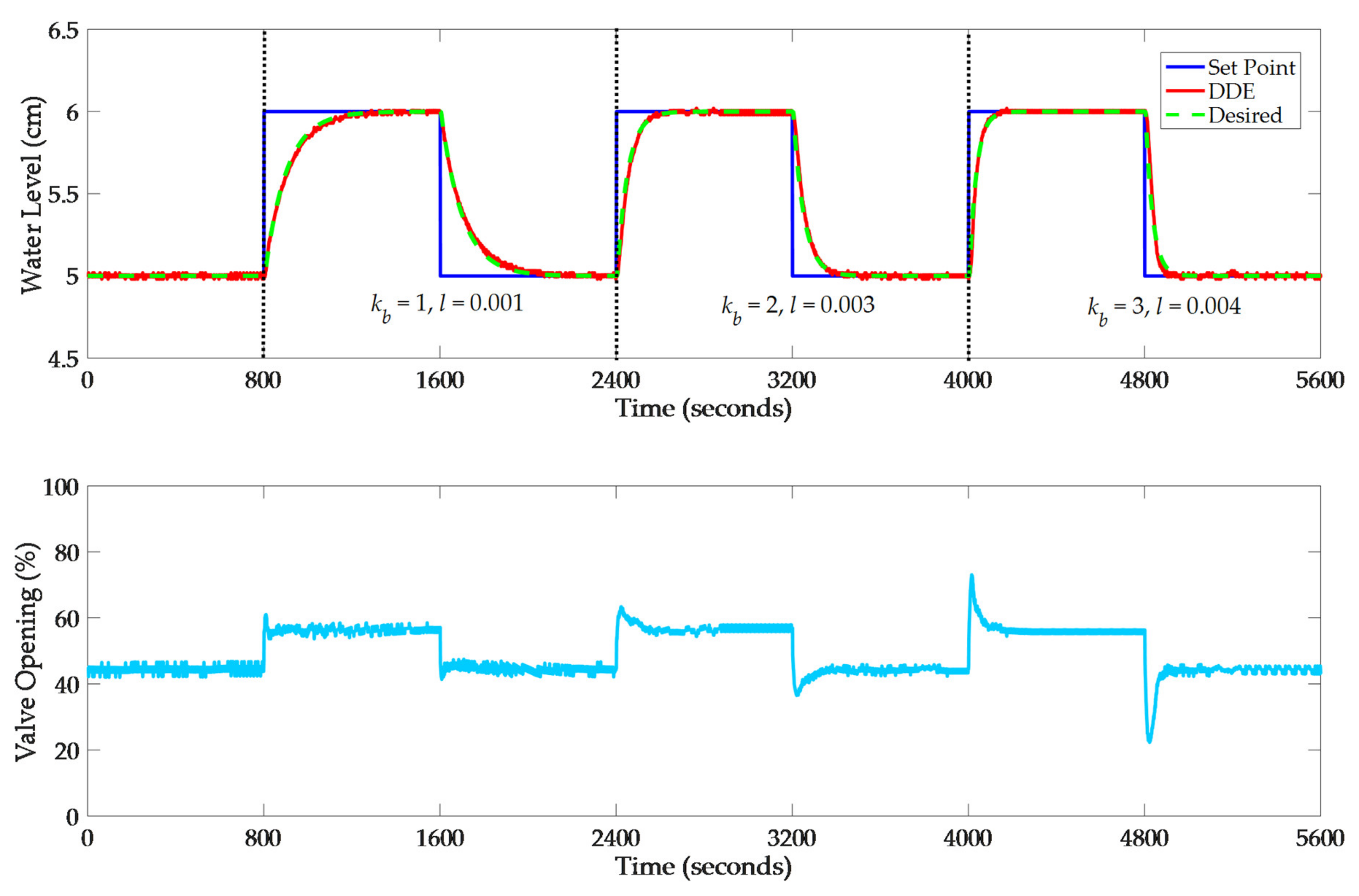
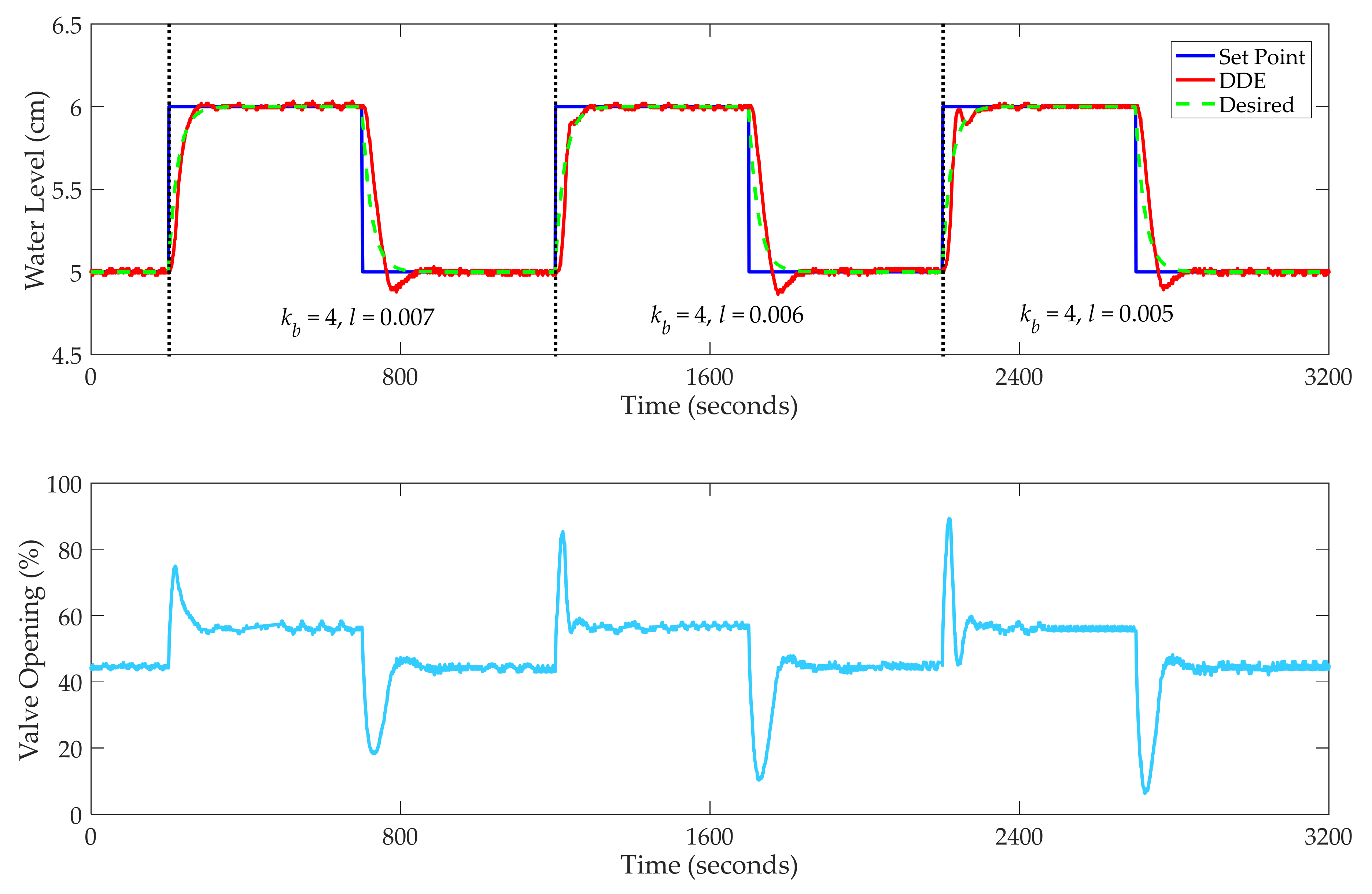
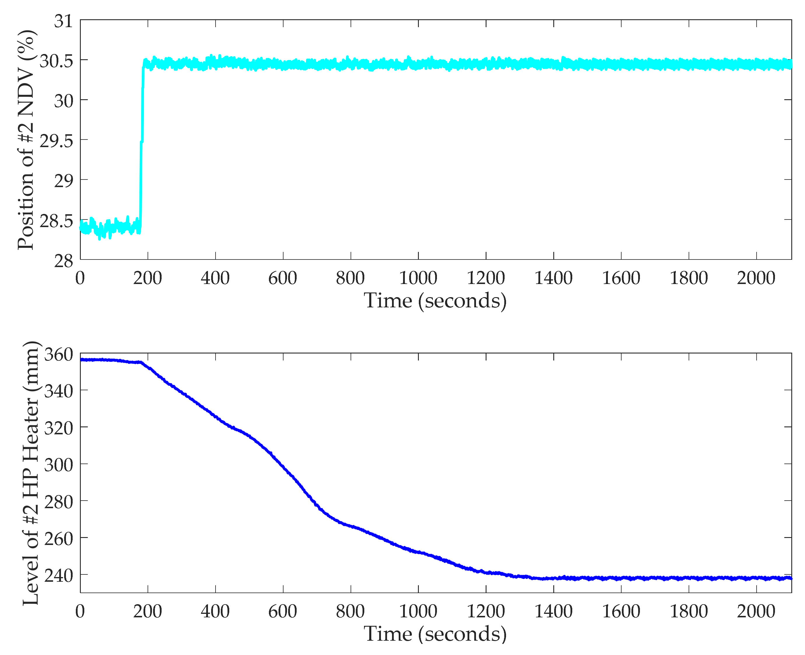
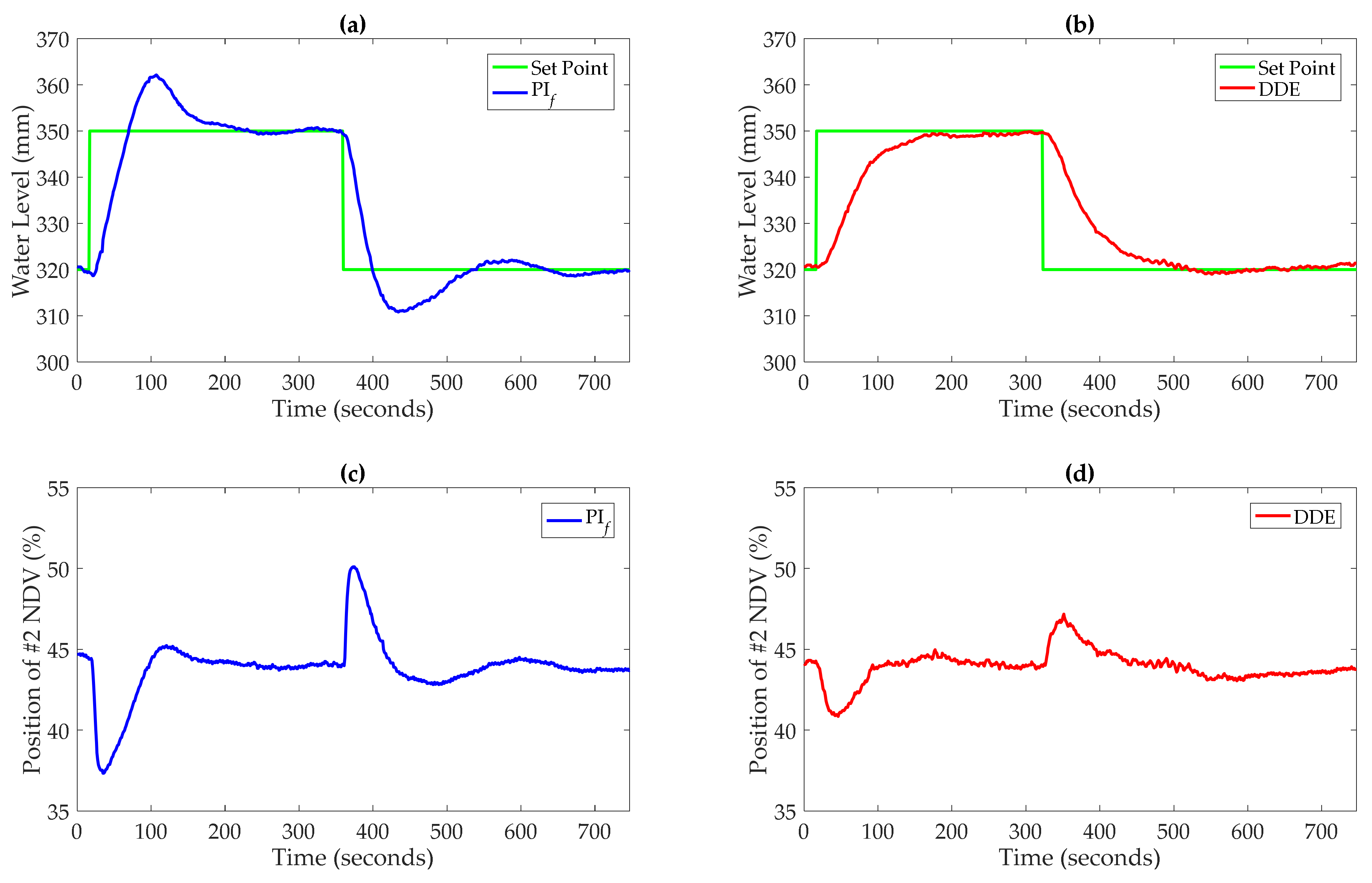
7.2. Results and Discussion of Field Tests

All field tests were carried out from 5:06 p.m. to 9:30 p.m. on 2 September 2021. The variation of the load is illustrated in Figure 31.
From Figure 31, it is easy to learn that the load varied between 495 MW and 525 MW, which is higher than 300 MW. Similar to Section 6.2, DDE PI was designed based on the proposed selection procedure. The level of the HP heater is a nonlinear process as well, such that the controller will obtain a different performance when the set point has a positive step change and a negative step change. Consequently, the closed-loop output of DDE PI should satisfy all the criteria in Section 4.2 when the level set point increases and decreases.
During the field tests, the parameter kb was augmented from 1 by a step of 1, and the absolute value of l was reduced from 1.3 by a step of 0.1. Figure 32 and Figure 33 show the field test results of the DDE PIs when kb = 1, 2, 3, 4 and 5. Note that the level set point varied between 320 mm and 350 mm.
According to Figure 32 and Figure 33, it is evident that the closed-loop output of DDE PI can track the desired dynamic response accurately with almost no overshoot when l is tuned appropriately. In addition, obvious oscillation and actuator saturation are nonexistent. To quantitatively evaluate whether all criteria were satisfied, the dynamic indices of the DDE PIs with kb = 1, 2, 3, 4 and 5 are presented in Table 8.
According to Table 8, obviously, the overshoots and IAE errors of the DDE PIs with kb = 1, 2, 3, 4 and 5 satisfied Criterion 1 and Criterion 2, respectively. As a result, the closed-loop output of DDE PI can track the desired dynamic response accurately when kb = 1, 2, 3, 4 and 5.
However, if kb is augmented to six, the closed-loop output of DDE PI may be unable to track the desired dynamic response accurately with the tuning parameters. Figure 34 illustrates the field test results of DDE PI with kb = 6.
From Figure 34, if the level set point increases from 320 mm to 350 mm, the error between the closed-loop output of DDE PI and the desired dynamic response became apparent when kb = 6 and l = −0.5. However, when the absolute value of l was reduced to 0.4, the actuator had severe oscillation when the level set point decreased. Table 9 lists the field test dynamic indices of DDE PI with kb = 6 to evaluate whether the closed-loop output could track the desired dynamic response accurately.
According to Table 9, when l = −0.5 and −0.4, the overshoot and the IAE error were larger than 1% and 10%, respectfully, if the level set point increased from 320 mm to 350 mm. Therefore, based on all the criteria in Section 4.2, the limit of ωd existed between 5ωd0 and 6ωd0.
Then, DDE PI with kb = 5 was compared with the original PI controller, which was tuned by an experienced field engineer such that kp = −2/9 and ki = −1/297. Figure 35 and Figure 36 illustrate the comparisons of the reference tracking performance and disturbance rejection performance, respectfully, between DDE PI and the original PI, which is denoted as “PIf”. The level set point was regulated between 320 mm and 350 mm, and disturbances in the position of EDV #2 with an amplitude of ±2% were added.
From the results of the field tests, in terms of reference tracking, DDE PI had a more moderate tracking performance than PIf. Moreover, if EDV #2 came into service, DDE PI could reject the disturbance with a smaller dynamic deviation than PIf. As a result, a well-tuned DDE PI has superiorities in both reference tracking and disturbance rejection.
To quantitatively evaluate the performance of different PI controllers, Table 10 presents the dynamic indices. Note that e+ and e are denoted as the maximum positive and negative deviation, respectively.
From Table 10, it is easy to learn that DDE PI can largely improve the performance of the level control of the HP heater. The overshoot was smaller, and the settling time was shorter than before. Moreover, DDE PI can reject external disturbances more effectively.
The field tests confirmed the merit of the proposed desired dynamic selection procedure; that is, the desired dynamic equation can be designed based on the time scale of the process without using an accurate plant model, and the controller can obtain the fastest reference tracking speed under various constraints. The successful application of DDE PI to the level control of an HP heater indicates its promising prospect in the control of coal-fired power plants.

8. Conclusions

This paper studied the desired dynamic selection of an RM-based PID controller: DDE PID. According to the design, simulations, experiments and field tests, some concluding remarks about DDE PID are summarized as follows:
  • The desired dynamic equation of DDE PI or PID can be designed based on the time scale of the process without using an accurate plant model;
  • Constrained by the actuator and the process characteristics, in terms of fixed criteria, the limit of desired dynamic selection always exists;
  • The NP-hard problem of PID tuning can be eliminated by using the proposed selection procedure;
  • Tuned by the proposed method, DDE PID can obtain the fastest and moderate tracking performance and track its desired dynamic response accurately.
Moreover, the proposed desired dynamic selection procedure provided a convenient alternative to PID tuning for practitioners in thermal engineering because of the following:
  • Only the open-loop test is required to obtain the initial values of DDE PI or PID:
  • For a determined desired dynamic equation, only one controller parameter, l, needs to be tuned;
  • The practitioners who understand the fundamentals of two-degree-of-freedom (2-DOF) PI and PID can design DDE PI- and DDE PID-based on the proposed procedure.
The authors hypothesized that the desired dynamic equations of other RM-based controllers, such as the Tornambè controller (TC) and linear ADRC (LADRC), can be selected based on the core idea of the proposed procedure. Moreover, the proposed method can provide guidance for the RM design of the model reference adaptive control. These are worthy of studying in the future.
Our future work will focus on the following:
  • The theoretical criterion of tracking the desired dynamic response;
  • The development of an auto-tuning toolbox for DDE PID based on the proposed procedure;
  • DDE PID design for infinite-dimensional systems;
  • The desired dynamic selections of TC and LADRC.

Author Contributions

Conceptualization, D.L. and G.S.; methodology, D.L. and G.S.; software, G.S. and S.L. (Shaojie Liu); validation, G.S., Z.W. and S.L. (Shaojie Liu); formal analysis, G.S.; investigation, G.S.; resources, G.S.; data curation, G.S.; writing—original draft preparation, G.S.; writing—review and editing, G.S., Z.W., S.L. (Shaojie Liu), D.L. and Y.D.; visualization, G.S.; supervision, D.L., Y.D. and S.L. (Shangming Liu); project administration, D.L. and S.L. (Shangming Liu); funding acquisition, D.L. and S.L. (Shangming Liu). All authors have read and agreed to the published version of the manuscript.

Funding

This research was funded by the National Science and Technology Major Project of China, 2017-V-0005-0055, the National Natural Science Foundation of China under Grant No. 52106030 and the Science & Technology Research Project in Henan Province of China under Grant No. 212102311052.

Institutional Review Board Statement

Not applicable.

Informed Consent Statement

Not applicable.

Data Availability Statement

Not applicable.

Acknowledgments

Special thanks go to the State Power Investment Corporation (SPIC) Chaoyang Yanshanhu Power Co. Ltd. for the support of the field test platform. The first author, the third author, the corresponding author and the fifth author would like to thank the financial support provided by the State Key Lab of Power Systems in the Department of Energy and Power Engineering at Tsinghua University. Moreover, the second author would like to thank the support from the National Natural Science Foundation of China under Grant No. 52106030 and the Science & Technology Research Project in Henan Province of China under Grant No. 212102311052.

Conflicts of Interest

The authors declare no conflict of interest.

Appendix A

In this appendix, the asymptotic stability of DDE PI/PID is analyzed as follows.
By substituting Equation (7) for Equation (5) and defining the state vector X = [x1, x2]T, the state-space expression of the closed-loop system can be rewritten as
X ˙ = A X + E f ˜ ,
where
A = 0 1 h 0 h 1 , E = 0 1 ,
Note that A is the Routh–Hurwitz criterion. Construct the Lyapunov function of Equation (A1) as V 2 t = X T P X , where P is a positive definite matrix which satisfies A T P + P A = I . Then, the following is true:
V ˙ 2 t = X ˙ T P X + X T P X ˙                     = X T A T P + P A X + 2 E T P X f ˜                     = X 2 + 2 E T P X f ˜                     X 2 + γ E T P X 2 + f ˜ 2 γ
where γ is positive. By defining λmin(P) and λmax(P) as the maximum and minimum eigenvalue of P, respectively, then
λ min P X 2 V 2 t λ max P X 2 ,
Thus, V2(t) satisfies
V ˙ 2 t 1 λ max P V 2 t + γ λ max P λ min P V 2 t + f ˜ 2 γ ,
Let γ < λ min P λ 2 max P and define
N 1 = 1 λ max P γ λ max P λ min P ,
Then, Equation (A5) can be rewritten as
V ˙ 2 t N 1 V 2 t + f ˜ 2 γ = N 1 V 2 t + 2 γ V 1 t ,
Therefore, the following is true for any tt0:
V 2 t e N 1 t V 2 t 0 + 2 γ t 0 t e N 1 t τ V 1 τ d τ 0 lim t V 2 t 2 γ lim t t 0 t e N 1 τ V 1 τ d τ e N 1 t = 2 γ lim t V 1 t N 1
According to Equation (A8), it is easy to learn that lim t V 2 t = 0 since lim t V 1 t = 0 when k→∞. Consequently, the closed-loop system with DDE PID is asymptotically stable. In particular, the asymptotic stability of DDE PI can be analyzed based on above procedure.

Appendix B

In this appendix, the derivation of the critical gain is detailed. According to Equation (4), it is obvious that the critical gain l ˜ is the gain between y n and u.
In terms of DDE PI, the plant is regarded as a general first-order system. Therefore, the open-loop response of the process can be approximated as the response of Equation (28). The critical gain should be evaluated by the gain between y ˙ and u. Then, for the open-loop stable system, its differential equation model can be depicted as
y ˙ t = 1 T y t + K T u t τ ,
From Equation (A9), the gain between y ˙ and u is K/T. Aside from that, for the open-loop unstable system, the differential plant model can be depicted as
y ˙ t = K u t τ ,
According to Equation (A10), the gain between y ˙ and u is K. As a result, l ˜ can be evaluated by Equation (29) for DDE PI.
As for DDE PID, the plant is considered a general second-order system. Consequently, the open-loop response of the process can be approximated as the response of Equation (30). The critical gain should be evaluated by the gain between y ¨ and u. Then, for an open-loop stable system, its differential equation model can be depicted as
y ¨ t = T 1 + T 2 T 1 T 2 y ˙ t 1 T 1 T 2 y t + K T 1 T 2 u t τ ,
From Equation (A11), the gain between y ˙ and u is K/(T1T2). In addition, for the open-loop unstable system, the differential plant model can be depicted as
y ¨ t = 1 T 2 y ˙ t + K T 2 u t τ ,
According to Equation (A12), the gain between y ˙ and u is K/T2. As a result, l ˜ can be evaluated by Equation (31) for DDE PID.

Appendix C

Table A1. Dynamic indices of different controllers for 10 typical processes.
kbControllerσ (%)Ts (s)IAEsp 1IAEud 2
Gp1(s)Z-N59.612.350.470.34
IMC14.360.980.261.30
SIMC23.001.580.361.45
AMIGO5.561.570.570.99
DDE00.480.180.02
Gp2(s)Z-N55.791.870.470.08
IMC11.031.600.360.31
SIMC25.071.330.350.07
AMIGO4.452.230.750.27
DDE1.000.780.390.04
Gp3(s)Z-N029.626.886.80
IMC16.7423.155.334.40
SIMC19.4622.295.244.23
AMIGO3.8216.764.924.65
DDE0.0410.254.801.91
Gp4(s)Z-N65.052.980.620.06
IMC15.681.340.390.19
SIMC42.232.370.450.02
AMIGO6.052.100.770.17
DDE00.730.290.01
Gp5(s)Z-N66.67290.7168.909.96
IMC12.69151.6742.7033.45
SIMC4.05121.1143.3739.53
AMIGO0.19366.31156.6349.63
DDE0.56121.1268.2213.14
Gp6(s)Z-N62.1535.167.023.14
IMC10.6812.493.6012.90
SIMC12.0420.063.454.16
AMIGO1.9921.4310.709.25
DDE0.9910.975.491.34
Gp7(s)Z-N18.289.632.721.45
IMC15.1211.083.222.04
SIMC10.9014.413.372.20
AMIGO5.5414.095.012.57
DDE0.456.633.561.07
Gp8(s)Z-N68.2917.233.230.19
IMC21.9210.671.540.02
SIMC36.3415.263.130.54
AMIGO31.0628.284.975.90
DDE0.012.430.820.01
Gp9(s)SIMC37.6168.5911.5910.58
DDE021.277.230.45
Gp10(s)Z-N55.044.271.000.62
IMC11.8811.181.321.60
SIMC42.148.001.450.74
DDE01.730.570.06
1 IAEsp = IAE of reference tracking. 2 IAEud = IAE of disturbance rejection.

References

  1. Wu, Z.; He, T.; Liu, Y.; Li, D.; Chen, Y. Physics-informed energy-balanced modeling and active disturbance rejection control for circulating fluidized bed units. Control Eng. Pract. 2021, 116, 104934. [Google Scholar] [CrossRef]
  2. Lin, B. China Energy Outlook 2020; Peking University Press: Beijing, China, 2020. [Google Scholar]
  3. Minorsky, N. Directional stability of automatically steered bodies. Am. Soc. Nav. Eng. 1922, 34, 280–309. [Google Scholar] [CrossRef]
  4. Richalet, J.; Rault, A.; Testud, J.; Papon, J. Model predictive heuristic control: Applications to industrial processes. Automatica 1978, 14, 413–428. [Google Scholar] [CrossRef]
  5. Qin, S.J.; Badgwell, T.A. A survey of industrial model predictive control technology. Control Eng. Pract. 2003, 11, 733–764. [Google Scholar] [CrossRef]
  6. Han, J. From PID to active disturbance rejection control. IEEE Trans. Ind. Electron. 2009, 56, 900–906. [Google Scholar] [CrossRef]
  7. Gao, Z. Scaling and bandwidth-parameterization based controller tuning. In Proceedings of the American Control Conference, Denver, CO, USA, 4–6 June 2003; pp. 4989–4996. [Google Scholar]
  8. Wu, Z.; Gao, Z.; Li, D.; Chen, Y.; Liu, Y. On transitioning from PID to ADRC in thermal power plants. Control Theory Technol. 2021, 19, 3–18. [Google Scholar] [CrossRef]
  9. Shi, G.; Wu, Z.; He, T.; Li, D.; Ding, Y.; Liu, S. Decentralized active disturbance rejection control design for the gas turbine. Meas. Control. 2020, 53, 1589–1601. [Google Scholar] [CrossRef]
  10. Sun, L.; You, F. Machine learning and data-driven techniques for the control of smart power generation systems: An uncertainty handling perspective. Engineering 2021, 7, 1239–1247. [Google Scholar] [CrossRef]
  11. Sun, L.; Xue, W.; Li, D.; Zhu, H.; Su, Z. Quantitative tuning of active disturbance rejection controller for FOPDT model with application to power plant control. IEEE Trans. Ind. Electron. 2021, 69, 805–815. [Google Scholar] [CrossRef]
  12. Sun, L.; Li, D.; Lee, K.Y. Optimal disturbance rejection for PI controller with constraints on relative delay margin. Control Eng. Pract. 2016, 63, 103–111. [Google Scholar] [CrossRef]
  13. Wu, Z.; Li, D.; Xue, Y. A new PID controller design with constraints on relative delay margin for first-order plus dead time systems. Processes 2019, 7, 713. [Google Scholar] [CrossRef] [Green Version]
  14. O’Dwyer, A. Handbook of PI and PID Controller Tuning Rules; Imperial College Press: London, UK, 2009. [Google Scholar]
  15. Ziegler, J.G.; Nichols, N.B. Optimum settings for automatic controllers. Am. Soc. Mech. Eng. 1942, 64, 759–765. [Google Scholar] [CrossRef]
  16. Rivera, D.E.; Morari, M.; Skogestad, S. Internal model control. 4. PID control design. Ind. Eng. Chem. Process. Des. Dev. 1986, 25, 252–265. [Google Scholar] [CrossRef]
  17. Skogestad, S. Simple analytic rules for model reduction and PID controller tuning. J. Process Control 2003, 13, 291–309. [Google Scholar] [CrossRef] [Green Version]
  18. Åström, K.J.; Panagopoulos, H.; Hägglund, T. Design of PI controllers based on non-convex optimization. Automatica 1998, 34, 585–601. [Google Scholar] [CrossRef]
  19. Panagopoulos, H.; Åström, K.J.; Hägglund, T. Design of PID controllers based on constrained optimization. In Proceedings of the American Control Conference, San Diego, CA, USA, 2–4 June 1999; pp. 3858–3862. [Google Scholar]
  20. Jia, Y.; Zhang, R.; Lv, X.; Zhang, T.; Fan, Z. Research on temperature control of fuel-cell cooling system based on variable domain fuzzy PID. Processes 2022, 10, 534. [Google Scholar] [CrossRef]
  21. Shan, Y.; Zhang, L.; Ma, X.; Hu, X.; Hu, Z.; Li, H.; Du, C.; Meng, Z. Application of the modified fuzzy-PID-Smith predictive compensation algorithm in a pH-controlled liquid fertilizer system. Processes 2022, 9, 1506. [Google Scholar] [CrossRef]
  22. Li, D.; Gao, F.; Xue, Y.; Lu, C. Optimization of decentralized PI/PID controllers based on genetic algorithm. Asian J. Control 2007, 9, 306–316. [Google Scholar] [CrossRef]
  23. Killingsworth, N.J.; Krstic, M. PID tuning using extremum seeking: Online, model-free performance optimization. IEEE Control. Syst. Mag. 2006, 26, 70–79. [Google Scholar]
  24. Shouran, M.; Alsseid, A. Particle swarm optimization algorithm-tuned fuzzy cascade fractional order PI-fractional order PD for frequency regulation of dual-area power system. Processes 2022, 10, 477. [Google Scholar] [CrossRef]
  25. Shi, G.; Gao, Z.; Chen, Y.; Li, D.; Ding, Y. A controller design method for high-order unstable linear time-invariant systems. ISA Trans. 2022; in press. [Google Scholar] [CrossRef] [PubMed]
  26. Somefun, O.A.; Akingbade, K.; Dahunsi, F. The dilemma of PID tuning. Annu. Rev. Control. 2021, 52, 65–74. [Google Scholar] [CrossRef]
  27. He, T. Active Disturbance Rejection Control Design and Application in Thermal Energy System. Ph.D. Thesis, Tsinghua University, Beijing, China, 28 October 2019. [Google Scholar]
  28. Wang, W.; Li, D.; Gao, Q.; Wang, C. A two-degree-of-freedom PID controller tuning method. J. Tsinghua Univ. 2008, 48, 1962–1966. [Google Scholar]
  29. Shi, G.; Li, D.; Ding, Y.; Chen, Y. Desired dynamic equational proportional-integral-derivative controller design based on probabilistic robustness. Int. J. Robust Nonlinear Control 2021. [Google Scholar] [CrossRef]
  30. Wang, W.; Li, D.; Xue, Y. Decentralized two degree of freedom PID tuning method for MIMO processes. In Proceedings of the IEEE International Symposium on Industrial Electronics, Seoul, Korea, 5–8 July 2009; pp. 143–148. [Google Scholar]
  31. Zhang, M.; Wang, J.; Li, D. Simulation analysis of PID control system based on desired dynamic equation. In Proceedings of the 8th World Congress on Intelligent Control and Automation, Jinan, China, 7–9 July 2010; pp. 3638–3644. [Google Scholar]
  32. Xue, Y.; Li, D.; Liu, J. DDE-based PI controller and its application to gasifier temperature control. In Proceedings of the International Conference on Control, Automation and Systems, Gyeonggi-do, Korea, 27–30 October 2010; pp. 2194–2197. [Google Scholar]
  33. Donghai Li, M.; Zhu, M.; Sun, L. Desired dynamic equation based PID control for combustion vibration. J. Low Freq. Noise Vib. Act. Control 2015, 34, 107–117. [Google Scholar] [CrossRef] [Green Version]
  34. Hu, Z.; Li, D.; Jiang, X.; Wang, J. Desired-dynamics-based design of control strategy for multivariable system with time delays. In Proceedings of the International Conference on Computer Application and System Modeling, Taiyuan, China, 22–24 October 2010; pp. 191–196. [Google Scholar]
  35. Wang, X.; Yan, X.; Li, D.; Sun, L. An approach for setting parameters for two-degree-of-freedom PID controllers. Algorithm 2018, 11, 48. [Google Scholar] [CrossRef] [Green Version]
  36. Guo, L. On critical stability of discrete-time adaptive nonlinear control. IEEE Trans. Autom. Control 1997, 42, 1488–1499. [Google Scholar]
  37. Xie, L.; Guo, L. How much uncertainty can be dealt with by feedback. IEEE Trans. Autom. Control 2000, 45, 2203–2217. [Google Scholar]
  38. Tornambè, A.; Valigi, P. A decentralized controller for the robust stabilization of a class of MIMO dynamical systems. J. Dyn. Syst. Meas. Control 1994, 116, 293–304. [Google Scholar] [CrossRef]
  39. Wu, Z.; Shi, G.; Li, D.; Liu, Y.; Chen, Y. Active disturbance rejection control design for high-order integral systems. ISA Trans. 2021, in press. [Google Scholar] [CrossRef]
  40. Cheng, X.; Wu, Z.; Li, D.; Zhu, M. Acoustic impedance tuning with active disturbance rejection control. J. Low Freq. Noise Vib. Act. Control 2018, 37, 1109–1124. [Google Scholar] [CrossRef] [Green Version]
  41. Khalil, H.K. Nonlinear Systems; Prentice-Hall: Upper Saddle River, NJ, USA, 1996; pp. 111–180. [Google Scholar]
  42. Luo, J.; Zhang, X.; Li, D.; Hu, Y. Tuning of PID controller for unstable plant systems. J. Xi’an Univ. Technol. 2015, 31, 475–481. [Google Scholar]
  43. Dorf, R.C.; Bishop, R.H. Modern Control Systems, 13th ed.; Pearson Education, Inc.: New York, NY, USA, 2017; p. 835. [Google Scholar]
  44. Jin, Y. Process Control; Tsinghua University Press: Beijing, China, 1993; pp. 26–27. (In Chinese) [Google Scholar]
  45. Yang, X. Automatic Control. for Thermal Process, 2nd ed.; Tsinghua University Press: Beijing, China, 2008; pp. 124–125. (In Chinese) [Google Scholar]
  46. Wu, Z.; Yuan, J.; Liu, Y.; Li, D.; Chen, Y. An active disturbance rejection control design with actuator rate limit compensation for the ALSTOM gasifier benchmark problem. Energy 2021, 227, 120447. [Google Scholar] [CrossRef]
  47. Koszaka, L.; Rudek, R.; Pozniak-Koszalka, I. An idea of using reinforcement learning in adaptive control systems. In Proceedings of the International Conference on Networking, International Conference on Systems and International Conference on Mobile Communications and Learning Technologies, Washington, DC, USA, 23–29 April 2006; p. 190. [Google Scholar]
  48. Åström, K.J.; Hägglund, T. Advanced PID Control; ISA-The Instrumentation, Systems, and Automation Society: Research Triangle Park, NC, USA, 2006. [Google Scholar]
  49. Ray, L.R.; Stengel, R.F. A Monte Carlo approach to the analysis of control system robustness. Automatica 1993, 29, 229–236. [Google Scholar] [CrossRef]
  50. Shi, G.; Liu, S.; Li, D.; Ding, Y.; Chen, Y. A controller synthesis method to achieve independent reference tracking performance and disturbance rejection performance. ACS Omega 2022, 7, 16164–16186. [Google Scholar] [CrossRef]
  51. Sun, L.; Li, D.; Hu, K.; Lee, K.Y.; Pan, F. On tuning and practical implementation of active disturbance rejection controller: A case study from a regenerative heater in a 1000 MW power plant. Ind. Eng. Chem. Res. 2016, 55, 6686–6695. [Google Scholar] [CrossRef]
  52. Zhao, Y.; Wang, C.; Liu, M.; Chong, D.; Yan, J. Improving operational flexibility by regulating extraction steam of high-pressure heaters on a 660 MW supercritical coal-fired power plant: A dynamic simulation. Appl. Energy 2018, 212, 1295–1309. [Google Scholar] [CrossRef]
  53. Wang, Z.; Pang, H. High water level automatic control logic optimization based on the least square method. Control. Eng. China 2018, 25, 897–902. [Google Scholar]
Figure 1. The structure of DDE PI/PID.
Processes 10 01059 g001
Figure 2. The influence of k and l on the control performance of DDE PID.
Processes 10 01059 g002
Figure 3. Open-loop step responses of processes.
Processes 10 01059 g003
Figure 4. Illustration of Criterion 1.
Processes 10 01059 g004
Figure 5. Illustration of Criterion 2.
Processes 10 01059 g005
Figure 6. Illustration of Criterion 3.
Processes 10 01059 g006
Figure 7. Illustration of Criterion 4.
Processes 10 01059 g007
Figure 8. A flow chart of the desired dynamic selection procedure.
Processes 10 01059 g008
Figure 9. Control performance of DDE PID with different kb for Gp1(s).
Processes 10 01059 g009
Figure 10. Control performance of DDE PID with different kb for Gp8(s).
Processes 10 01059 g010
Figure 11. Control performance of DDE PID with different kb for Gp10(s).
Processes 10 01059 g011
Figure 12. Control performance of DDE PID with different kb for Gp4(s).
Processes 10 01059 g012
Figure 13. Control performance of DDE PID with different kb for Gp7(s).
Processes 10 01059 g013
Figure 14. Control performance of DDE PID with different kb for Gp9(s).
Processes 10 01059 g014
Figure 15. Control performance of different PID controllers: (a,c) Gp1(s) and (b,d) Gp2(s).
Processes 10 01059 g015
Figure 16. Control performance of different PID controllers: (a,c) Gp3(s) and (b,d) Gp4(s).
Processes 10 01059 g016
Figure 17. Control performance of different PID controllers: (a,c) Gp5(s) and (b,d) Gp6(s).
Processes 10 01059 g017
Figure 18. Control performance of different PID controllers: (a,c) Gp7(s) and (b,d) Gp8(s).
Processes 10 01059 g018
Figure 19. Control performance of different PID controllers: (a,c) Gp9(s) and (b,d) Gp10(s).
Processes 10 01059 g019
Figure 20. Results of Monte Carlo trials of different PID controllers: (a) Gp1(s), (b) Gp2(s), (c) Gp3(s), (d) Gp4(s), (e) Gp5(s) and (f) Gp6(s).
Processes 10 01059 g020
Figure 21. Results of Monte Carlo trials of different PID controllers: (a) Gp7(s), (b) Gp8(s), (c) Gp9(s) and (d) Gp10(s).
Processes 10 01059 g021
Figure 22. The schematic structure of the experimental set-up.
Processes 10 01059 g022
Figure 23. Result of open-loop step test of the water tank.
Processes 10 01059 g023
Figure 24. Experimental results of DDE PIs with kb = 1, 2 and 3.
Processes 10 01059 g024
Figure 25. Experimental results of DDE PIs with kb = 4.
Processes 10 01059 g025
Figure 26. Simulation results of different PI controllers based on the identified transfer function model.
Processes 10 01059 g026
Figure 27. Experimental results of Z-N PI and SIMC PI: (a,c) Z-N PI and (b,d) SIMC PI.
Processes 10 01059 g027
Figure 28. Experimental results of AMIGO PI and DDE PI: (a,c) AMIGO PI and (b,d) DDE PI.
Processes 10 01059 g028
Figure 29. The structure of the HP steam extraction and drainage system. (IP = intermediate pressure, LP = low pressure, EDV = emergency drainage valve, NDV = normal drainage valve, M/A = manual/auto).
Processes 10 01059 g029
Figure 30. The results of the open-loop step test (date: 31 August 2021; time span: 11:00 a.m. to 11:35 a.m.).
Processes 10 01059 g030
Figure 31. The variation of the load (date: 2 September 2021; time span: 5:06 p.m. to 9:30 p.m.).
Processes 10 01059 g031
Figure 32. The field test results of DDE PIs with kb = 1, 2 and 3 (date: 2 September 2021; time span: 5:06:00 p.m. to 6:24:52 p.m.).
Processes 10 01059 g032
Figure 33. The field test results of DDE PIs with kb = 4 and 5 (date: 2 September 2021; time span: 6:24:53 p.m. to 6:50:06 p.m.).
Processes 10 01059 g033
Figure 34. The field test results of DDE PIs with kb = 6 (date: 2 September 2021; time span: 7:11:00 p.m. to 7:30:12 p.m.).
Processes 10 01059 g034
Figure 35. The comparison of reference tracking performance between PIf and DDE PI: (a,c) PIf and (b,d) DDE PI (date: 2 September 2021; time span: DDE PI = 6:37:02 p.m. to 6:49:29 p.m.; PIf = 7:30:13 p.m. to 7:42:40 p.m.).
Processes 10 01059 g035
Figure 36. The comparison of disturbance rejection performance between PIf and DDE PI: (a,c) PIf and (b,d) DDE PI (date: 2 September 2021; time span: DDE PI = 8:49:49 p.m. to 8:59:29 p.m.; PIf = 9:09:34 p.m. to 9:19:14 p.m.).
Processes 10 01059 g036
Table 1. Transfer function models of 10 typical industrial processes.
ProcessTypeTransfer Function Model
Gp1(s)Low-Order System 1 s   +   1 0.2 s   +   1
Gp2(s)High-Order System 2 15 s   +   1 20 s   +   1 s   +   1 0.1 s   +   1 2
Gp3(s) 1 s   +   1 4
Gp4(s) 1 s   +   1 0.2 s   +   1 0.04 s   +   1 0.008 s   +   1
Gp5(s)Dead Time System e 20 s 160 s   +   1
Gp6(s) e s 20 s   +   1 2 s   +   1
Gp7(s)Non-Minimum Phase System 0.3 s   +   1 0.08 s   +   1 2 s   +   1 s   +   1 0.4 s   +   1 0.2 s   +   1 0.05 s   +   1
Gp8(s)Integral System 0.17 s   +   1 2 s s   +   1 2 0.028 s   +   1
Gp9(s) 1 s 2 s   +   1
Gp10(s)Unstable System 4 4 s 1 s   +   1
Table 2. Limits of ωd for 10 typical processes without the consideration of actuator saturations.
ProcessPI/PID-b 1tp (s)τ (s)ωd0kb*Limit of ωd 2
Gp1(s)PID-b4.1401.411>16>16ωd0
Gp2(s)PID-b51.7500.113>50>50ωd0
Gp3(s)PID-b9.101.50.7680.90.9ωd0~ωd0
Gp4(s)PID-b4.1901.3945.15.1ωd0~5.2ωd0
Gp5(s)PI-b644.53200.0062.92.9ωd0~3ωd0
Gp6(s)PID-b79.7110.0745.35.3ωd0~5.4ωd0
Gp7(s)PID-b10.121.470.6751.21.2ωd0~1.3ωd0
Gp8(s)PID-b2.3802.454>16>16ωd0
Gp9(s)PID-b2.1102.7680.10.1ωd0~0.2ωd0
Gp10(s)PID-b1.6603.518>16>16ωd0
1 PI-b or PID-b is denoted as DDE PI or PID. 2 Limit of ωd: “d0~d0” means that the limit exists between d0 and d0, while “>d0” means that the limit may not be determined by the characteristics of the process.
Table 3. Parameters of different PID controllers for 10 typical processes.
ProcessPI/PID-bZ-N
{kp, Ti, Td}
IMC
{kp, Ti, Td}
SIMC
{kp, Ti, Td}
AMIGO
{kp, Ti, Td, b}
DDE
{ωd0, kb, l}
Gp1(s)PID-b{13.2, 0.2, 0.05}{8.46, 1.1, 0.05}{5, 0.8, 0.1}{5.15, 0.44, 0.047, 5.15} {1.411, 8, 28.2}
Gp2(s)PID-b{5.6, 0.3, 0.075}{3.59, 1.05, 0.075}{6.67, 0.4, 0.15}{2.23, 0.53, 0.072, 2.23}{0.113, 50, 70.5}
Gp3(s)PID-b{0.72, 5, 1.25}{0.46, 1.5, 1.25}{0.5, 1.5, 1}{0.47, 2.08, 0.83, 0}{0.768, 0.9, 6.3}
Gp4(s)PID-b{8.92, 0.30, 0.074}{5.72, 1.1, 0.074}{17.9, 0.23, 0.22}{3.54, 0.54, 0.071, 3.54}{1.394, 5.1, 25.2}
Gp5(s)PI-b{7.2, 66.67, 0}{4.99, 170, 0}{4, 160, 0}{2.16, 106.64, 0, 2.16}{0.006, 2.9, 0.042}
Gp6(s)PID-b{12.6, 4, 1}{8.07, 21, 1}{10, 8, 2}{4.93, 8.59, 0.97, 4.93}{0.074, 5.3, 0.159}
Gp7(s)PID-b{2.04, 2.94, 0.74}{1.31, 2.5, 0.74}{1.3, 2, 1.2}{0.97, 2.21, 0.62, 0.97}{0.675, 1.2, 5.6}
Gp8(s)PID-b{3.82, 1.81, 0.45}{23.20, 1.90, 1.33}{1.4, 2.86, 1.33}{0.45, 13.52, 0.085, 0}{2.454, 1, 1.4}
Gp9(s)PID-bN/A *N/A{0.0625, 8, 8}N/A{2.768, 0.1, 1.9}
Gp10(s)PID-b{9.6, 1, 0.25}{15.31, 4.9, 0.73}{8.93, 0.8, 0.8}N/A{3.518, 1, 5.1}
* N/A = not applicable.
Table 4. Experimental dynamic indices of DDE PIs with kb = 1, 2 and 3.
kblΔr (cm) *σ (%)ΔIAE (%)
10.001from 5 to 60.647.94
from 6 to 50.649.29
20.003from 5 to 60.646.81
from 6 to 50.647.29
30.004from 5 to 60.645.87
from 6 to 50.647.11
* The variation of the level set point, where “from 5 to 6” means the set point varied from 5 cm to 6 cm while “from 6 to 5” means the set point varied from 6 cm to 5 cm.
Table 5. Experimental dynamic indices of DDE PIs with kb = 4.
kblΔr (cm)σ (%)ΔIAE (%)
40.007from 5 to 63.2015.39
from 6 to 512.1819.07
0.006from 5 to 61.9213.53
from 6 to 513.4617.98
0.005from 5 to 60.6412.51
from 6 to 510.9016.44
Table 6. Parameters of different PI controllers for level control of the water tank.
Z-N
{kp, Ti}
IMC
{kp, Ti}
SIMC
{kp, Ti}
AMIGO
{kp, Ti, b}
DDE
{ωd0, kb, l}
{17.46, 16.67}{158.12, 99.5}{131.08, 40}{81.56, 41.45, 81.56} {0.0103, 3, 0.004}
Table 7. Dynamic indices of different PI controllers for the level control of the water tank.
Controllerσ (%)Ts (s)emax (cm)
Z-N35.2610230.42
IMCN/AN/AN/A
SIMC172.44N/AN/A
AMIGO1.921230.20
DDE0.64870.20
Table 8. Field test dynamic indices of DDE PIs with kb = 1, 2, 3, 4 and 5.
kblΔr (mm) *σ (%)ΔIAE (%)
1−0.1from 320 to 3500.849.72
from 350 to 3200.732.88
2−0.2from 320 to 3500.740.28
from 350 to 3200.659.89
3−0.3from 320 to 3500.454.91
from 350 to 3200.834.69
4−0.3from 320 to 35009.94
from 350 to 32004.89
5−0.4from 320 to 3500.320.40
from 350 to 3200.432.10
* The variation of the level set point, where “from 320 to 350” means the set point varied from 320 mm to 350 mm, while “from 350 to 320” means the set point varied from 350 mm to 320 mm.
Table 9. Field test dynamic indices of DDE PIs with kb = 6.
kblΔr (mm)σ (%)ΔIAE (%)
6−0.5from 320 to 3503.7511.13
from 350 to 32004.96
−0.4from 320 to 3501.1010.43
from 350 to 3205.048.22
Table 10. Field test dynamic indices of different PI controllers.
ControllerΔr (mm)σ (%)Ts (s)e+ (mm)e (mm)
PIffrom 320 to 35040.3317515.7613.17
from 350 to 32030.53243
DDEfrom 320 to 3500.321388.548.41
from 350 to 3200.43143
Publisher’s Note: MDPI stays neutral with regard to jurisdictional claims in published maps and institutional affiliations.

