
Design Framework and Laboratory Experiments for Helix and Slinky Type Ground Source Heat Exchangers for Retrofitting Projects


 ,
,
Abstract
:1. Introduction
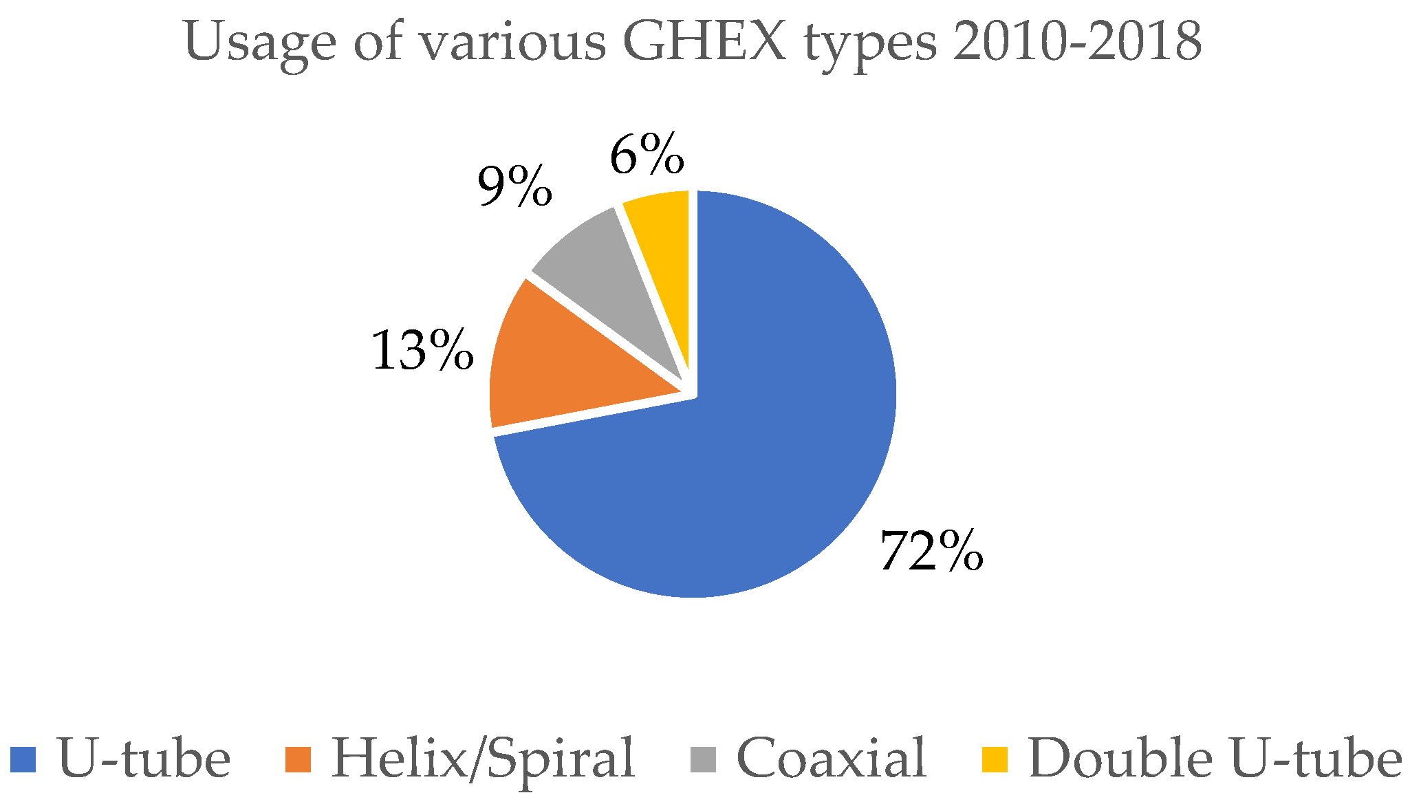
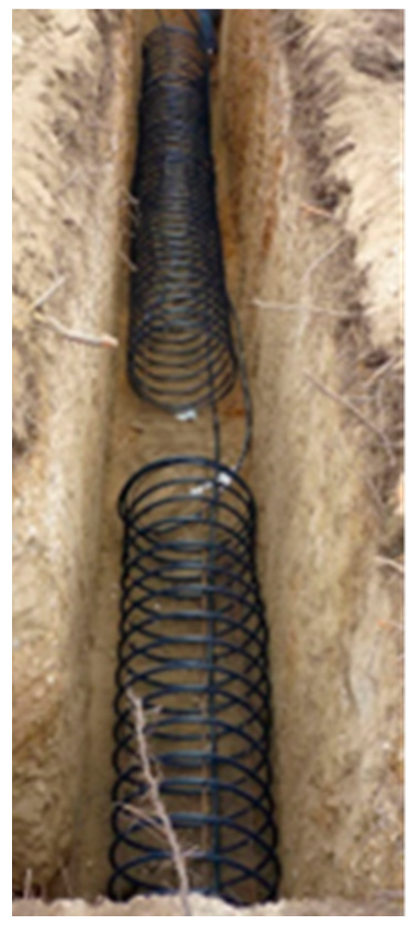
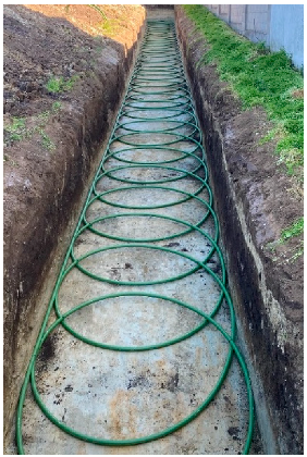
1.1. Shallow Heat Exchanger Types
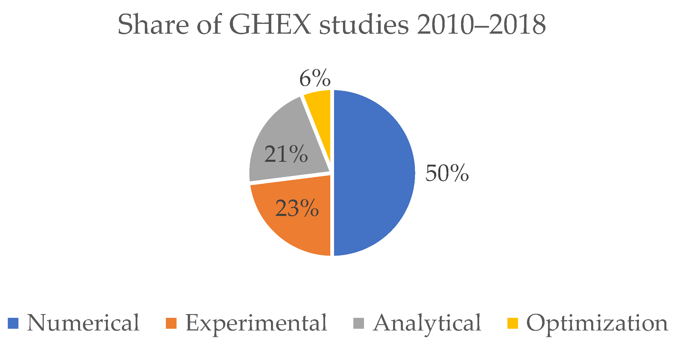
1.2. Tools Available for GHEX Design
- List of compared software:
- EED: Earth Energy Designer, BLOCON AB, https://buildingphysics.com (accessed on 10 April 2022)
- GHLEPRO: Ground Loop Heat Exchanger Design Software, https://hvac.okstate.edu (accessed on 10 April 2022)
- EWS: ErdWärmeSonden, Huber Energietechnik AG, EWS|Huber Energietechnik AG, Zurich (hetag.ch) accessed on 10 April 2022)
- GLD: Ground Loop Design, Thermal Dynamics, www.groundloopdesign.com (accessed on 10 April 2022)
- FEFLOW: Finite Element subsurface FLOW system, DHI, www.feflow.info (accessed on 10 April 2022)
- SBM: Superposition Borehole Model for TRNSYS
- DST: Duct Storage Model for TRNSYS
- COMSOL: Multiphysics Simulation Software, COMSOL, www.comsol.de (accessed on 10 April 2022)
- G-functions:
2. Materials and Methods
2.1. Materials
2.2. Methods
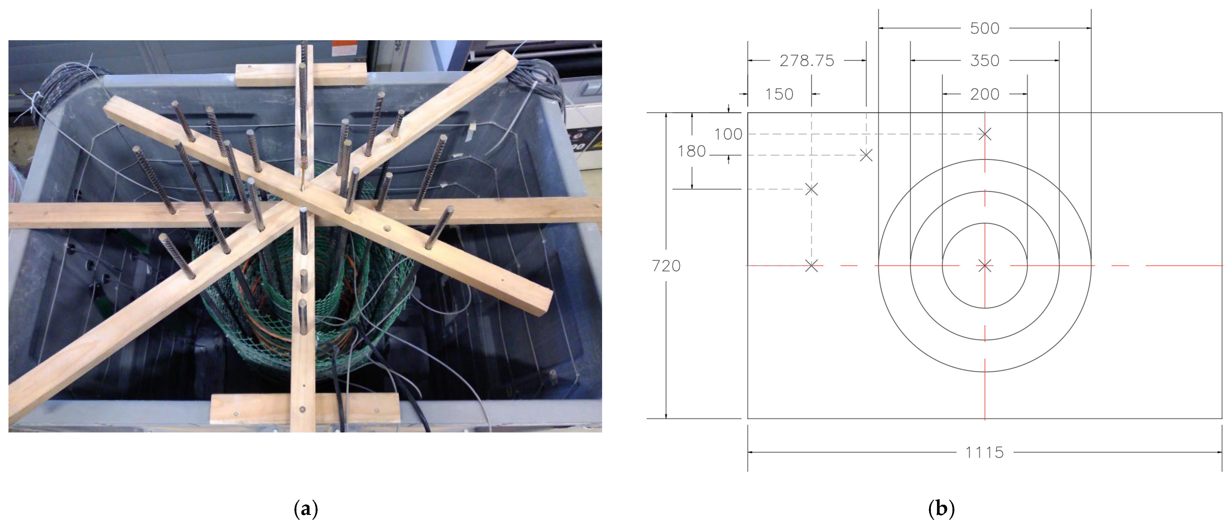
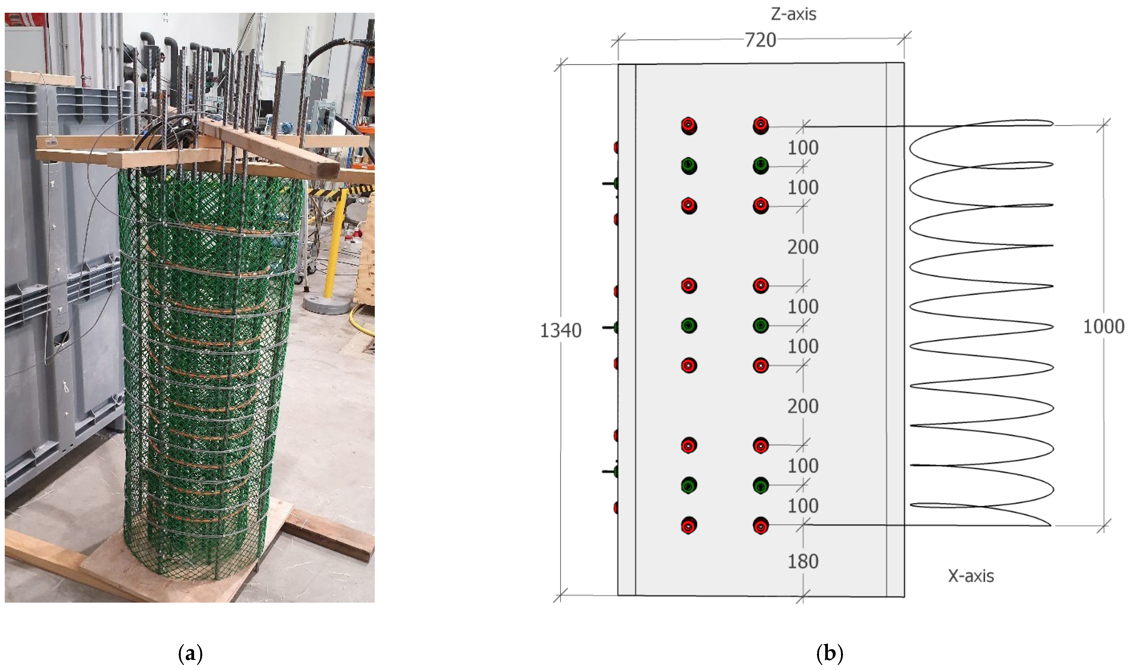
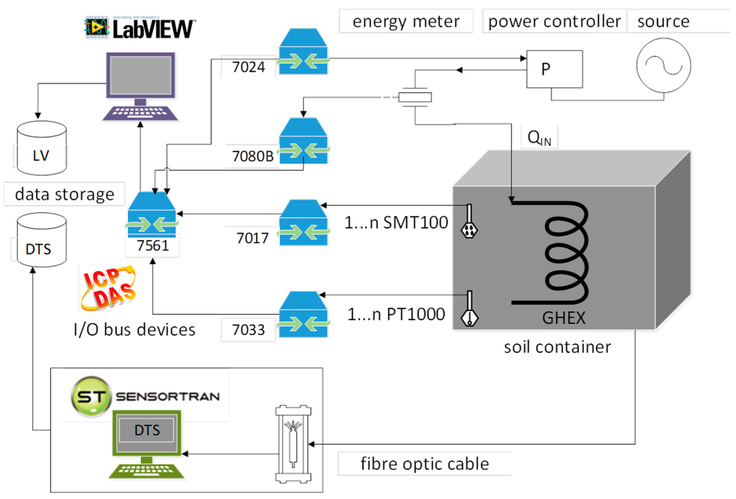
2.2.1. Data Acquisition
2.2.2. Material Properties
3. Results
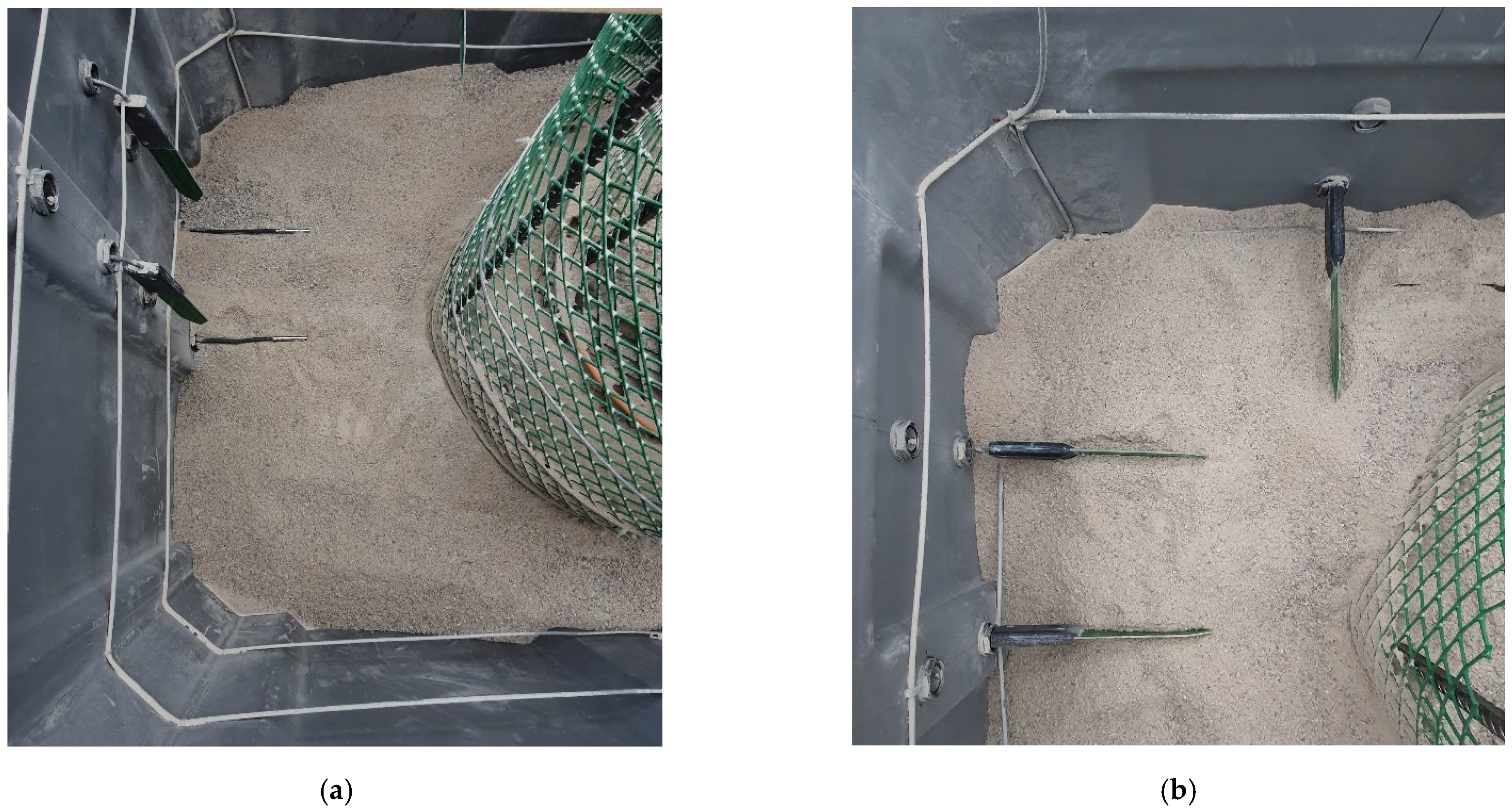
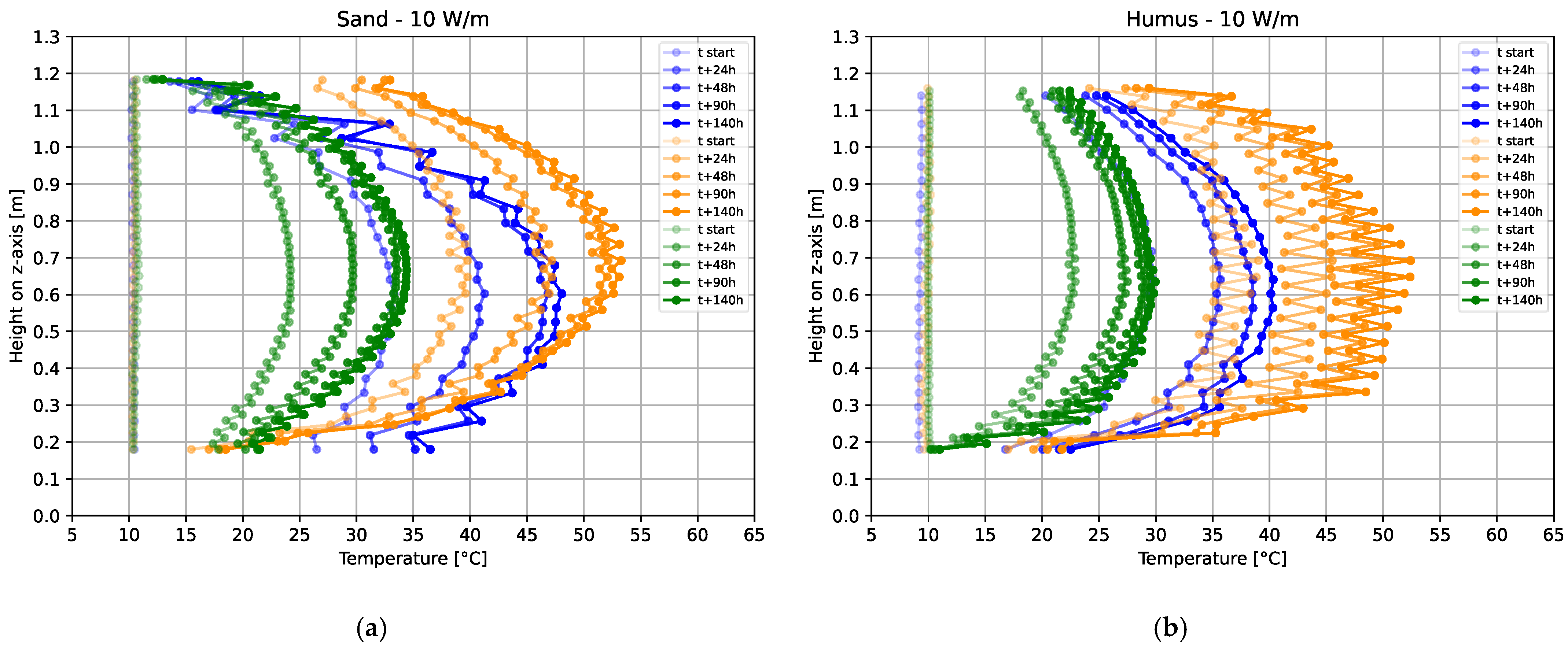
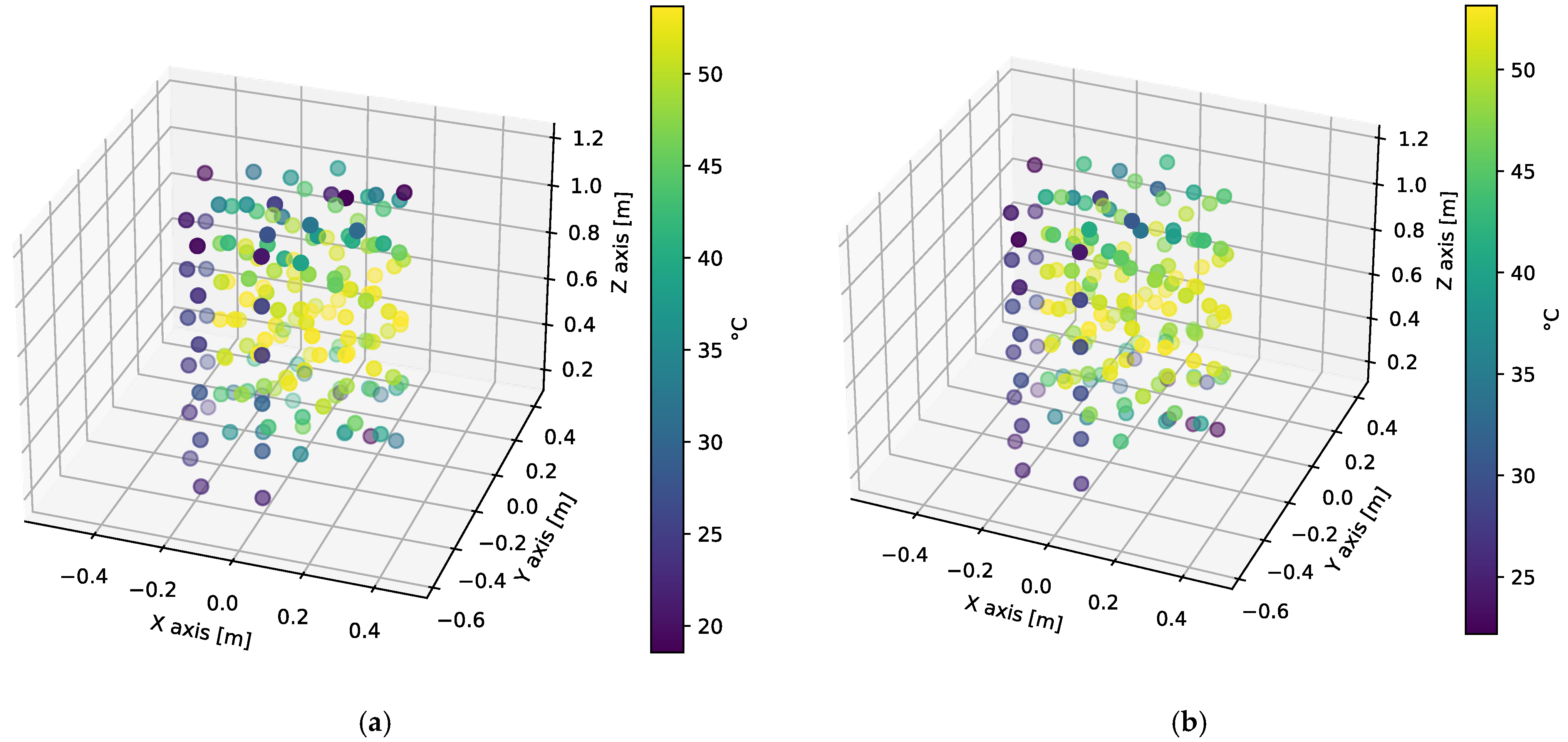
3.1. Experimental
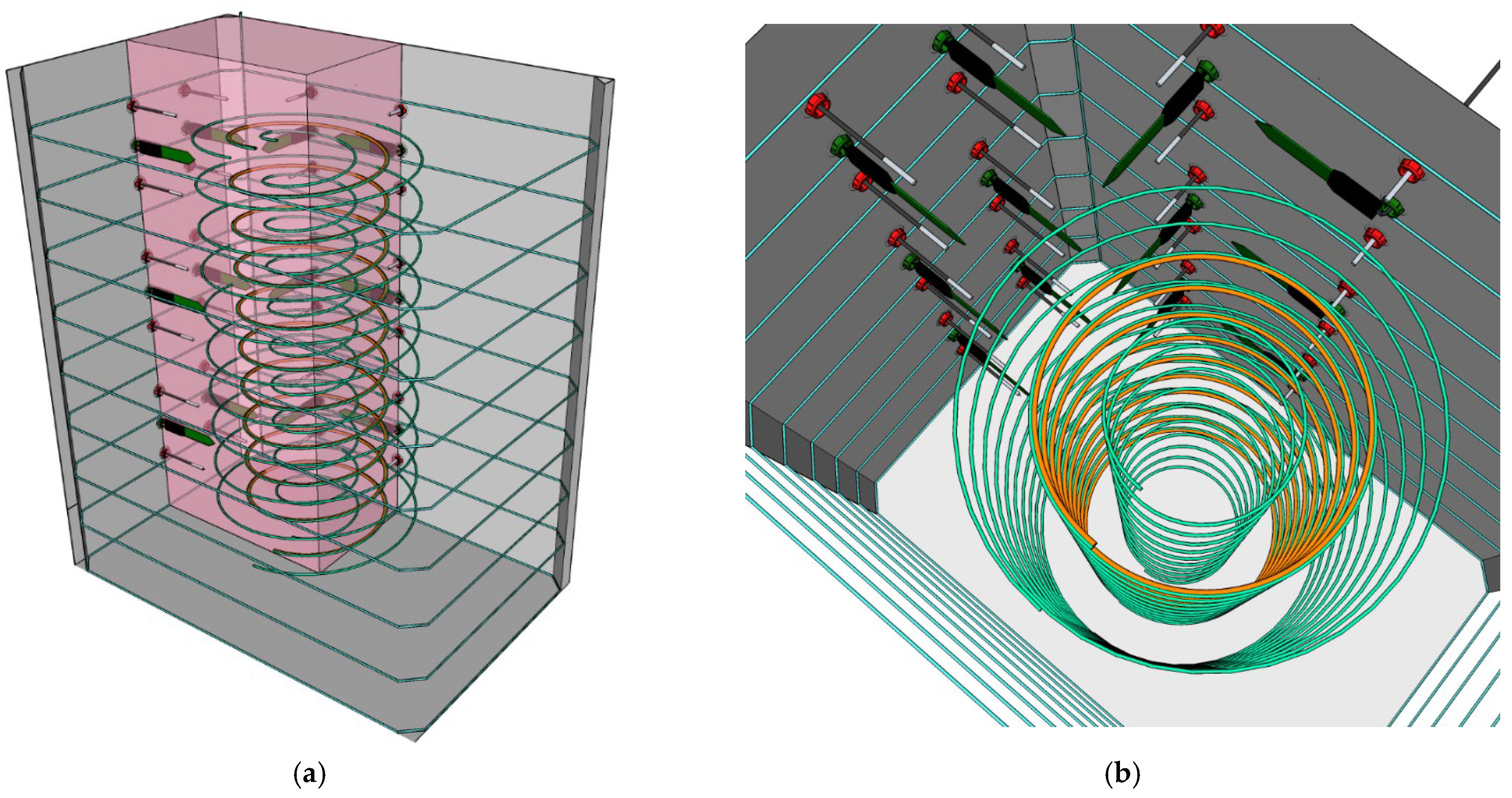
- Geometry of helix: h = 1 m, d = 0.35 m, p = 0.1 m
- Specific heating rate: 10 W/m–113.1 W total
- Soil type: Sand (a) and soil (b); untreated H2O content
- Ambient temperature: 10 °C as starting condition
3.2. Material Data
3.3. CFD
4. Discussion
5. Summary and Conclusions
Author Contributions
Funding
Data Availability Statement
Acknowledgments
Conflicts of Interest
References
- GEOFIT Project. 2018. Available online: https://geofit-project.eu/ (accessed on 10 April 2022).
- Sanner, B. Current status of ground source heat pumps in Europe. In Proceedings of the 9th International Conference on Thermal Energy Storage Futurestock 2003, Warsaw, Poland, 1–4 September 2003. [Google Scholar]
- Nowak, T.; Westring, P. European Heat Pump Market and Statistics Report. 2019. European Heat Pump Association, Rue d’Arlon 63-67, B-1040 Brussels. Available online: www.ehpa.org (accessed on 10 April 2022).
- Javadi, H.; Mousavi, A.; Rosen, M.A.; Pourfallah, M. Performance of ground heat exchangers: A comprehensive review of recent advances. Energy 2019, 178, 207–233. [Google Scholar] [CrossRef]
- Sanner, B.; Hellström, G.; Spitler, J.; Gehlin, S. Thermal Response Test—Current Status and World-Wide Application. In Proceedings of the World Geothermal Congress, Antalya, Turkey, 24–29 April 2005. [Google Scholar]
- ISO 17628; Geotechnical Investigation and Testing—Geothermal Testing—Determination of Thermal Conductivity of Soil and Rock Using a Borehole Heat Exchange. The European Committee for Standardization: Brussels, Belgium, 2015.
- Spitler, J.D. GLHEPRO—A Design Tool for Commercial Building Ground Loop Heat Exchangers. In Proceedings of the Fourth International Heat Pumps in Cold Climates Conference, Québec, ON, Canada, 17–18 August 2000. [Google Scholar]
- Jeon, J.S.; Lee, S.-R.; Kim, M.-J.; Yoon, S. Suggestion of a Scale Factor to Design Spiral-Coil-Type Horizontal Ground Heat Exchangers. Energies 2018, 11, 2736. [Google Scholar] [CrossRef] [Green Version]
- Solar Redl. 2019. Available online: https://www.solar-redl.de/ (accessed on 10 April 2019).
- Ringgrabenkollektor. 2022. Available online: http://www.ringgrabenkollektor.at/hauptseite.html (accessed on 12 April 2022).
- Nian, Y.-L.; Cheng, W.-L. Analytical g-function for vertical geothermal boreholes with effect of borehole heat capacity. Appl. Therm. Eng. 2018, 140, 733–744. [Google Scholar] [CrossRef]
- Saeidi, R.; Noorollahi, Y.; Esfahanian, V. Numerical simulation of a novel spiral type ground heat exchanger for enhancing heat transfer performance of geothermal heat pump. Energy Convers. Manag. 2018, 168, 296–307. [Google Scholar] [CrossRef]
- Witte, H.J.L. Development and validation of analytical solutions for earth basket (spiral) heat exchangers. Eur. Geotherm. Congr. 2022; submitted. [Google Scholar]


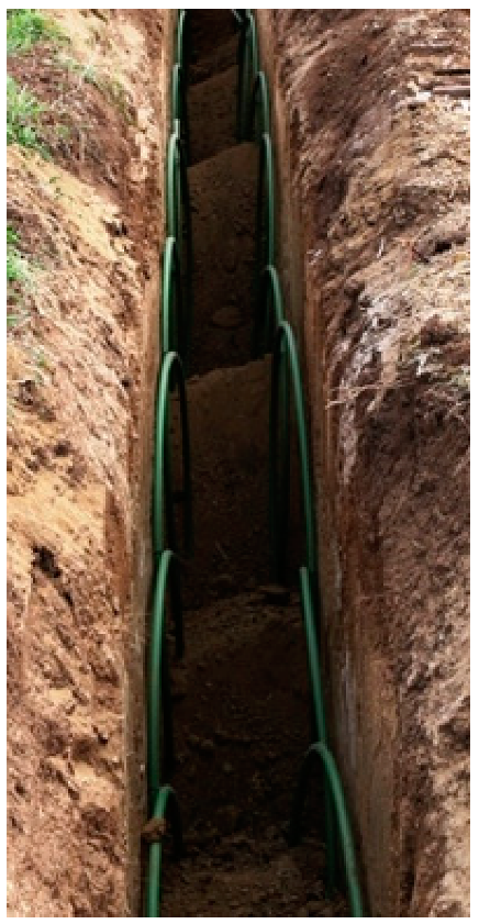
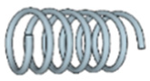
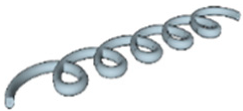
| Vertical Spiral/Helix [9] | Horizontal Spiral [9] | Horizontal Slinky-Loop [10] | Vertical Slinky-Loop [10] |
|---|---|---|---|
| Installation in vertical boreholes up to 5 m depth and a coil diameter of 0.2–0.5 m. | Installation in trenches up to 5 m depth and a coil diameter of 0.2–05 m. | Installation in trenches up to 2 m width and 1.5 m depth. The overlapping of the loops can range between no overlap and half of the diameter. | Installation in trenches about 0.5 m width |
 |  |  |  |
| Design Tool | EED | GHLEPRO | EWS | GLD | FEFLOW | SBM | DST | COMSOL |
|---|---|---|---|---|---|---|---|---|
| Analytical g-function | X | X | - | X | - | - | - | - |
| Numerical g-function | - | - | X | - | X | X | X | X |
| Arbitrary time step | - | - | - | ? | X | X | X | X |
| Conductive heat flow | X | X | X | X | X | X | X | X |
| Advective heat flow | - | - | - | - | X | - | - | X |
| Layered geology | - | - | - | - | X | - | partly | X |
| Arbitrary topology | - | - | - | X | X | X | - | X |
| Geometry Types | Vertical Helix | Horizontal Helix | Horizontal Flat-Slinky | Vertical Flat Helix |
|---|---|---|---|---|
 |  |  |  | |
| Soil types | Gravel/soil/mixture | |||
| Sand/Soil/50/50 | ||||
| Heat flow rates | Heat extraction | Heat injection | ||
| Sand | Soil | |||||||||||
|---|---|---|---|---|---|---|---|---|---|---|---|---|
| Dry < 0.1% | Moisture 6.14% | Dry < 0.1% | Moisture 6.24% | |||||||||
| T | cp | λ | ρ | cp | λ | ρ | cp | λ | ρ | cp | λ | ρ |
| °C | J/kgK | W/mK | kg/m³ | J/kgK | W/mK | kg/m³ | J/kgK | W/mK | kg/m³ | J/kgK | W/mK | kg/m³ |
| −10 | 0.889 | 0.3809 | 1822 | 1.070 | 1.2435 | 1928 | 0.913 | 0.3401 | 1942 | n.a. | 0.504 | 2004 |
| 0 | n.a. | 0.3784 | 1822 | n.a. | 0.9788 | 1928 | 0.966 | 0.3370 | 1942 | n.a. | 0.490 | 2004 |
| 10 | 0.947 | 0.3796 | 1822 | 1.095 | 0.9514 | 1928 | 0.974 | 0.3251 | 1942 | n.a. | 0.483 | 2004 |
| 20 | 0.941 | 0.3840 | 1822 | 1.152 | 0.9339 | 1928 | 1.006 | 0.3162 | 1942 | n.a. | 0.502 | 2004 |
| 25 | 0.962 | 0.3884 | 1822 | 1.100 | 0.9619 | 1928 | n.a. | 0.3121 | 1942 | n.a. | 0.509 | 2004 |
| 30 | 0.985 | 0.3874 | 1822 | 1.116 | 0.9728 | 1928 | 1.056 | 0.3068 | 1942 | n.a. | 0.515 | 2004 |
| 40 | 1.027 | 0.3896 | 1822 | 1.134 | 1.09 | 1928 | 1.086 | 0.2991 | 1942 | n.a. | 0.536 | 2004 |
| 50 | 1.065 | 0.3915 | 1822 | 1.139 | 1.19 | 1928 | 1.085 | 0.3058 | 1942 | n.a. | 0.552 | 2004 |
| 60 | 1.038 | 0.3929 | 1822 | 1.184 | 1.31 | 1928 | 1.072 | 0.3024 | 1942 | n.a. | 0.562 | 2004 |
| 70 | 1.061 | 0.3873 | 1822 | 1.295 | 1.46 | 1928 | 1.106 | 0.2972 | 1942 | n.a. | 0.566 | 2004 |
Publisher’s Note: MDPI stays neutral with regard to jurisdictional claims in published maps and institutional affiliations. |
© 2022 by the authors. Licensee MDPI, Basel, Switzerland. This article is an open access article distributed under the terms and conditions of the Creative Commons Attribution (CC BY) license (https://creativecommons.org/licenses/by/4.0/).
Share and Cite
Kling, S.; Haslinger, E.; Lauermann, M.; Witte, H.; Reichl, C.; Steurer, A.; Dörr, C. Design Framework and Laboratory Experiments for Helix and Slinky Type Ground Source Heat Exchangers for Retrofitting Projects. Processes 2022, 10, 959. https://doi.org/10.3390/pr10050959
Kling S, Haslinger E, Lauermann M, Witte H, Reichl C, Steurer A, Dörr C. Design Framework and Laboratory Experiments for Helix and Slinky Type Ground Source Heat Exchangers for Retrofitting Projects. Processes. 2022; 10(5):959. https://doi.org/10.3390/pr10050959
Chicago/Turabian StyleKling, Stephan, Edith Haslinger, Michael Lauermann, Henk Witte, Christoph Reichl, Alexander Steurer, and Constantin Dörr. 2022. "Design Framework and Laboratory Experiments for Helix and Slinky Type Ground Source Heat Exchangers for Retrofitting Projects" Processes 10, no. 5: 959. https://doi.org/10.3390/pr10050959
APA StyleKling, S., Haslinger, E., Lauermann, M., Witte, H., Reichl, C., Steurer, A., & Dörr, C. (2022). Design Framework and Laboratory Experiments for Helix and Slinky Type Ground Source Heat Exchangers for Retrofitting Projects. Processes, 10(5), 959. https://doi.org/10.3390/pr10050959