The Characteristic of High-Speed Centrifugal Refrigeration Compressor with Different Refrigerants via CFD Simulation

Abstract

This study used Computational Fluid Dynamics (CFD) to simulate and analyze the working fluid in magnetic centrifugal refrigerant compressors using R-134a to mixed refrigerant: R-513A and HFO (Hydrofluoroolefins) Hydrofluoroolefin refrigerant: R-1234yf, and the impact on integrated part-load performance, Integrated Part Load Value (IPLV) and internal flow field. This study used a single-stage 280 USRT maglev centrifugal refrigerant compressor as a simulation model. Three different refrigerants were used: R-134a, R-513A, and R-1234yf, as presented in the National Institute of Standards and Technology (NIST) real gas database. The refrigerant was used to set the IPLV working conditions and change the compressor speed and mass flow rate to simulate the compressor’s characteristic curve after replacing the refrigerant. The compressor working conditions were the fixed refrigeration cycle condensation and evaporation following the same capacity standards. This study used the CFD software by Ansys software company to simulate the flow field. The k-omega turbulence software was used to model the turbulence. The results show that the maglev centrifugal refrigerant compressor efficiency dropped significantly when the refrigerant was directly replaced. Based on R-134a, the full load efficiency of R-1234yf dropped 13.21%, the full load efficiency of R-513A dropped 9.97%, and the partial load efficiency was similar to R-134a.

1. Introduction

1.1. Development Overview of Magnetic Levitation Centrifugal Compressor

The present magnetic levitation centrifugal compressor has a smaller volume, lower noise, and lower starting current than conventional centrifugal compressors. The magnetic levitation centrifuge is the most efficient water chiller among the present air-conditioning systems because the magnetic bearing mechanical loss is much lower than the dynamic bearing mechanical loss. Wide-area volume control is achieved with a frequency converter speed control, IGV (inlet guide vane), and diffusion width regulation. The small operating range of the conventional fixed-frequency centrifugal compressor is improved. It is considered advantageous to replace water chillers with a displacement compressor.

However, the flow field variation inside the centrifugal compressor is complex. It is difficult to observe the internal flow field variation using instruments. Therefore, this study used CFD to simulate the magnetic levitation centrifugal refrigerant compressor Integrated Part Load Value (IPLV) using R-134a refrigerant. The simulation result was compared with the experimental results to validate the simulation result. HFO refrigerant was replaced with a working fluid for another simulation. This study used R-1234yf and R-513A refrigerant for simulation comparison analyses. The changes in the performance and flow field of the magnetic levitation centrifugal compressor after replacing the HFC refrigerant with HFO refrigerant are discussed.

1.2. Motivation and Objective

There are two methods for replacing the refrigerant: directly replacing the refrigerant and redesigning the compressor for the new refrigerant as shown in

Table 1. Cost comparison of direct refrigerant replacement and compressor redesign.

Change Refrigerant	Equipment Cost	Operating Cost
Direct replacement	Low	High
Redesign	High	Low

. Directly replacing the refrigerant may increase the equipment operation cost, while the redesign method will increase the original price of the equipment. This study focused on predicting the impact of directly replacing the existing R134a refrigerant with R-1234yf refrigerant and R-513A refrigerant. Using the results of this study, it can be judged whether it is necessary to redesign the compressor blades according to different refrigerants in the future. The purpose is to discuss the effect of direct refrigerant replacement on the high-speed centrifugal compressor.

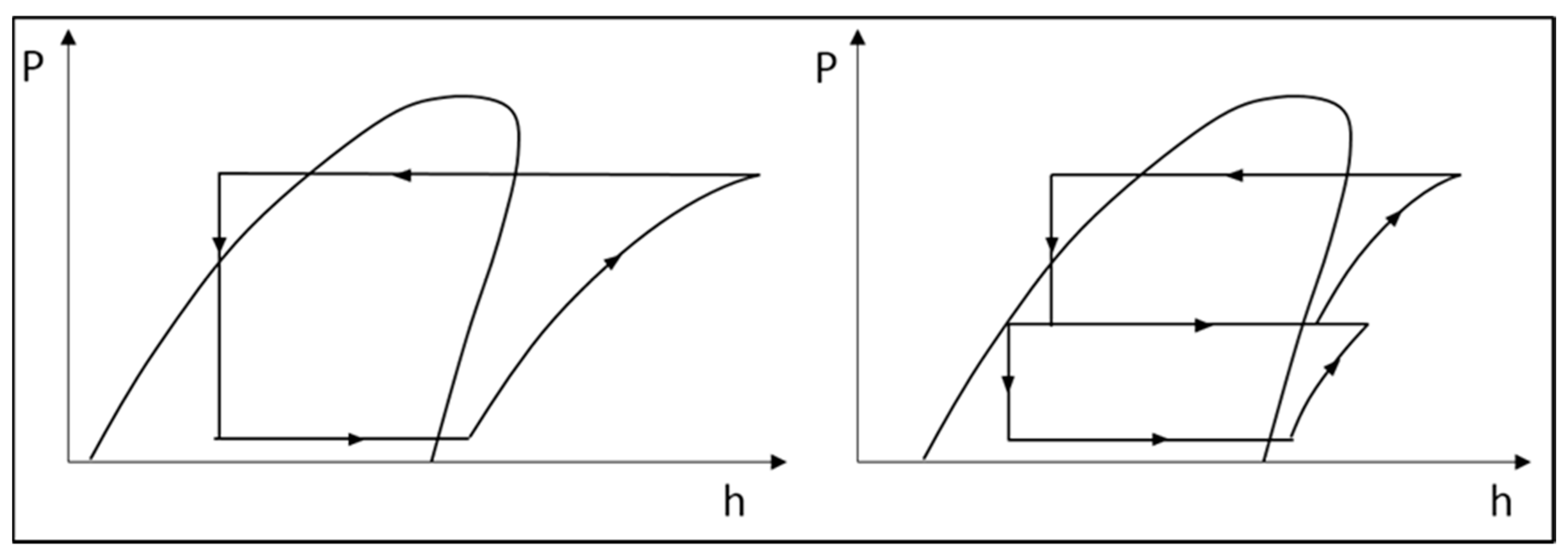
1.3. Magnetic Levitation Centrifugal Compressor Operating Principle

The magnetic levitation centrifugal compressor drives an impeller to rotate through a magnetic bearing. The refrigerant is sucked into the impeller through an inlet tube and radially delivered at high speed to the diffuser. The fluid’s dynamic energy is reduced by the diffuser and converted into pressure energy. This energy conversion occurs continuously at the volute casing. The chiller system’s required pressure ratio and mass flow rate are achieved by high-efficiency impeller compression. The flow field feature and performance effectiveness of flow elements are the keys to compressor performance.

In addition to the single-stage compression type magnetic levitation centrifugal compressor, this study discussed the compression/pressurization two-stage compression process. An economizer was arranged between every two compression process stages. The thermodynamic cycle diagrams are shown in Figure 1.

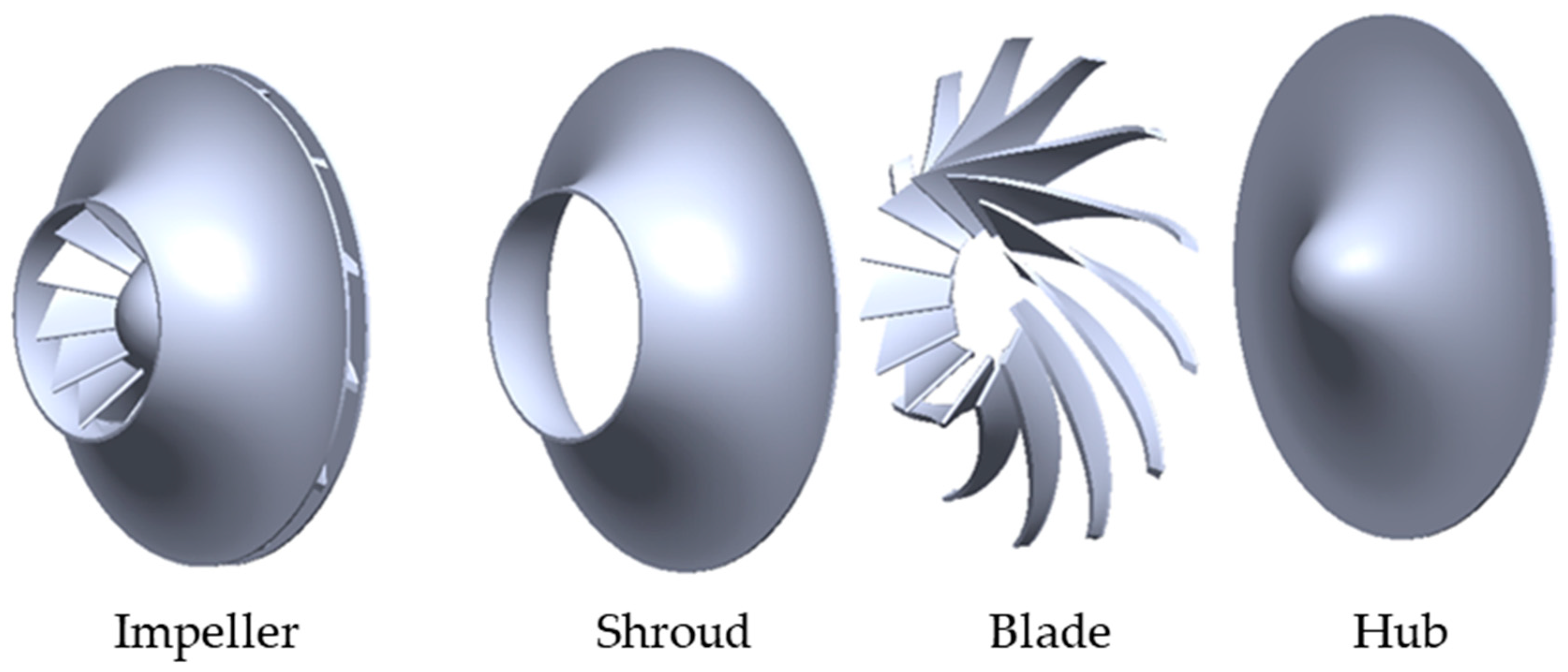
1.4. Magnetic Levitation Centrifugal Compressor Structure

The single-stage magnetic levitation centrifugal compressor contains four flow channel sections: 1. inlet zone, 2. impeller zone, 3. diffuser zone, and 4. volute zone:

• Inlet zone

The inlet zone is the area from the compressor inlet to the front end of an impeller. The inlet guide vanes (IGV) can be arranged in the inlet zone annularly, parallel to the refrigerant flow direction when they are not actuating. When the refrigerant flow needs to be reduced, the flow direction of the fluid entering the impeller is controlled by changing the blade angle. The fluid is pre-rotated to control the flow and regulate the refrigerating capacity in the water chiller. The inlet zone is free of IGV in this study, and the inlet nozzle was used instead.

2.

Impeller zone

The impeller zone is located downstream of the inlet zone. The impeller is driven by the magnetic levitation spindle motor to centrifugally discharge the refrigerant from the diffuser zone. The impeller is comprised of a Shroud, Blade, and Hub, as shown in Figure 2. As the rotation speed is not very high, the shroud will not influence the mechanical strength of the impeller. This study used an enclosed impeller to reduce the effect of leakage loss.

3.

Diffuser zone

There are Vaned and Vaneless Diffusers in the diffuser zone. The primary function is to transform the kinetic energy of the refrigerant at a high flow rate from the impeller into pressure energy. The diffuser form of the centrifugal compressor used in this study was a vaneless diffuser.

4.

Volute zone

The volute casing function is to collect the fluid from the diffuser or impeller zone and deliver it to the compressor outlet. The fluid kinetic energy is transformed into pressure energy in the process.

1.5. Adoption of Refrigerant

Montreal Protocol-Kigali Amendment [1] limits the use of R-134a refrigerant because the HFC refrigerant’s global warming potential (GWP) is as high as 1430. Due to an extensive discussion on the environmental considerations, the universally expected replaceable refrigerant is Hydrofluoroolefins (HFO) refrigerant. Its ozone depletion potential (ODP) is zero. Since its GWP is lower, it is a suitable substitute for HFC refrigerant [2]. The toxicity and flammability of R134a refrigerant, R1234yf refrigerant, R1234ze(E)refrigerant, and R513A refrigerant were compared according to the ASHRAE Standard 34-2019 [3] and shown in

Table 2. Refrigerant properties [3,4,5,6].

Refrigerant	R134a	R1234yf	R1234ze(E)	R513A
Type	HFC-134a	HFO-1234yf	HFO-1234ze	HFO-1234yf/HFC-134a (56/44)
Molar Mass (kg/kmol)	102.032	114.042	114.04	108.43
Critical Temperature (K)	374.26	367.85	382.51	368.06
Critical Pressure (kPa)	4059	3382.2	3634.9	3647.8
Critical Volume (m3/mol)	2.008 × 10−4	2.39808 × 10−4	2.043987 × 10−3	2.21092 × 10−4
Acentric Factor	0.326	0.276	0.313	-
Boling Temperature (K)	247.04	243.365	254.177	243.68
ODP	0	0	0	0
GWP100	1430	≤1	≤1	573
Safety Classifications	A1	A2L	A2L	A1

[3,4,5,6]. The definition and classification of safe levels are shown in

Table 3. Safety Classifications of ASHRAE Standard 34-2019 [3].

	Low Toxicity	High Toxicity
High Flammability	A3	B3
Low Flammability	A2	B2
	A2L	B2L
Nonflammable	A1	B1

[6].

R-1234yf refrigerant is currently the most popular refrigerant to replace R-134a refrigerant. Its working pressure and temperature are very close to that of R-134a refrigerant, and the GWP of R-1234yf refrigerant is mentioned in the literature [3]. The GWP100 of the refrigerant is re-estimated and its value is less than or equal to 1. However, at the same evaporation temperature the enthalpy difference of the R-1234yf refrigerant is small, and it can be expected that the R-1234yf refrigerant will have higher energy consumption in direct replacement.

R-513A refrigerant is an azeotropic refrigerant mixed with R-134a refrigerant and R-1234yf refrigerant. Referring to the research of Ian H. Bell et al. [6], its GWP100 is 573. At the same time, by mixing non-flammable R-134a refrigerant Mixed with R-1234yf refrigerant with safety grade-A2L is slightly flammable, and successfully reduced the flammability of the original R-1234yf to safety grade-A1.

R-1234ze(E) and R-1234ze(Z) belong to isomers, while for R-1234ze(Z), at the saturation temperature of 6.6 °C and 36.5 °C, the saturation pressure drops by 76% and 72%, which are much lower than that of R-134a refrigerant. While R-1234ze(E) refrigerant is a low pressure refrigerant, its saturation pressure at the same temperature, compared with R-134a refrigerant, at saturation temperature 6.6 °C and 36.5 °C, the saturation pressure drops by 26% and 25% (as shown in Figure 3). It is very difficult to estimate the feasibility of directly replacing the refrigerant, so this refrigerant will not be included in this study.

1.6. Part Load

Directly changing the working fluid influences water chiller performance to some extent. Appropriate volume control is necessary to change the refrigerant at a low replacement cost. The water chiller operation in most field domains is still a partial load. According to the IPLV computing Equation (1) in AHRI 551/591 [7], taking the operating time as a coefficient, the full load operating time coefficient is smaller than the operating time coefficient for each partial load. So, partial load efficiency is essential in water chiller operation.

IPLV (Integrated Part Load Value):

IPLV = 0.01A + 0.42B + 0.45C + 0.12D
A = COP at 100% load
B = COP at 75% load
C = COP at 50% load
D = COP at 25% load

(1)

1.7. Literature Review

1.7.1. References about Compressor

Adel Ghenaiet et al. [8] used the numerical simulation method to discuss the rotating stall of a centrifugal compressor. Using different assessment criteria, they found that the blockage factor and the adjusted load criterion were more suitable for predicting the stall starting position in the compressor.

Elkin I.GUTIÉRREZ VELÁSQUEZ [9] performed a correlation study on the main loss in the preliminary design of a centrifugal compressor. They showed that the efficiency prediction error would be as high as 8% if an incorrect loss correlation was used.

Zhang Chaowei et al. [10] created a new loss correlation method based on the centrifugal compressor air inlet speed relative Mach number and specific speed. This method is better than the conventional transonic centrifugal compressor setting method and is similar to the function of a subsonic centrifugal compressor.

Dongdong Zhao et al. [11] made an analysis model for the operational characteristics of a centrifugal compressor at different heights above sea level. They used a sliding mode controller to overcome air mass flow rate instability at high altitudes.

Changhee Kim et al. [12] used the CFX numerical simulation software of Ansys to simulate the differences between the centrifugal compressor in the steady-state and unsteady-state flow field. These differences were compared with the experimental result. They found that the three results were very similar, but at the design point, the steady-state simulation result was reduced by 4.15% compared with the total-to-static pressure ratio of the experimental result. The unsteady state simulation was reduced by 0.4%. Compared to the polytropic efficiency of the experimental result, the steady-state simulation result was reduced by 1.96%, and the unsteady state simulation result was reduced by 0.09%. The steady-state and unsteady-state flow fields had different Mach number and vortex distributions.

Hanzhi Zhang et al. [13] used experiments and numerical simulations to perform two-stage near surge point stall analyses for the centrifugal compressor with a vaneless diffuser. A partial stall occurred at the impeller’s eye at the early stage. Extensive back-flow occurred at the impeller’s eye at the late stage, leading to a loopful stall.

Rajiv Tiwari et al. [14] used visualization experiments and deep learning to change the flow and observe the pressure and flow field on the circumference of the outer casing of the centrifugal pump. They analyzed different degrees of blockage and cavitation to use a radial pressure sensor to predict the occurrence of blockage and cavitation.

Bernhard Semlitsch et al. [15] used numerical simulation and experimental validation to perform an unsteady-state analysis of the centrifugal compressor surge. They used sliding mesh at the impeller and found that in the flow field near the surge point, the back-flow generated upstream of the impeller formed swirls as the impeller rotated. The swirl significantly influenced the inflow angle and impeller efficiency.

J. Galindo et al. [16] used numerical simulation to perform simulation analyses of a centrifugal compressor and changed the inlet geometric features to observe the flow field variation when near surge flow and higher than design flow. They found that the convergent nozzle inlet had a better back-flow suppression effect in the surge flow. As the flow increased, the pressure loss induced by cross-section would reduce the efficiency.

1.7.2. References about Refrigerant

Ian H. Bell et al. [6] used simplified cycle simulation to perform a simulated comparison of 23 kinds of simple and mixed refrigerants. In an appropriate incombustible mixture, the R-513A refrigerant had the minimum GWP which was 537. The GWP was reduced by 54% compared with the R-134a refrigerant.

Jian Sun et al. [17] used a mathematical model of the refrigeration system to simulate the system capacity, available energy failure rate, energy efficiency, and available energy efficiency of R-134a and R-513A refrigerants at different ambient and space temperatures in the two-stage compression system using economizer. The result showed that at most, the system capacity was reduced by 12% after R-134a was replaced by R-513A refrigerant. The energy efficiency was reduced by 9% at most, and the available energy efficiency was reduced by 14% at most. The irreversibility was reduced at higher ambient temperature and space temperature by 5~13%. Whereas, at low temperatures, the reversible efficiency was increased by 3%.

Meng Yang et al. [18] experimentally replaced the R-134a refrigerant of a household refrigerator with R-513A refrigerant and compared the cooling rates resulting from the two refrigerants’ filling amounts in a 24-h energy consumption test and freezing test. The result showed that in the case of optimum refrigerant filling amount, the R-513 refrigerant cooling time was shortened by 21% compared with R-134a refrigerant. The 24-h energy consumption was reduced by 15%, and the freezing time was shorter. It indicated that the R-513A refrigerant could be used as a substitute for the household refrigerator, which uses R-134a refrigerant. The system’s redesign is unnecessary.

Adrián Mota-Babiloni et al. [19] used a miniature vapor compression system to test R-134a and R-513A refrigerants at different evaporating and condensing temperatures. They found that the R-513A refrigerant had a little higher available energy efficiency than the R-134a refrigerant. The compressor had the lowest available energy efficiency. The condenser and expansion valve had the highest available energy efficiency, whereas the available evaporator energy efficiency was median. Therefore, the R-134a can be directly replaced by an R-513A refrigerant in the miniature vapor compression system. Redesigning the system is unnecessary.

Velasco et al. [20] experimentally tested the performance difference between R-513A and R-134a refrigerants in the vapor compression refrigeration system with a micro-channel heat exchanger as a condenser. The experimental results showed that the energy efficiency ratio (EER) of the R-513A refrigerant was lower than R-134a refrigerant by 24% on average, and the R-513A refrigerant had a little lower isentropity and mechanical efficiency.

AliKhalid Shaker Al-Sayyab et al. [21] created a mathematical simulation to simulate a theoretical performance analysis of a solar-energy driven heat pump system with an ejector using R-134a, R-513A, and R-450A refrigerants. They found that the system using R-450A refrigerant had a higher COP.

V.Pérez-García et al. [22] tested R-134a, R-450A, and R-513A refrigerants in a system with an internal heat exchanger (IHX). They found that the R-513A refrigerant was the best choice for medium and low-temperature systems with IHX.

Chi-Chuan Wang [23] compared the two-phase R-1234yf refrigerant with R-134a refrigerant heat transfer performance according to the published documents and obtained multiple conclusions. The two refrigerants had a very slight HTC difference for in-tube convection boiling. For the same flow conditions (steam mass, mass velocity, saturation temperature, and caliber), the R-134a and R-1234yf refrigerants had the same flow pattern.

Zvonimir Janković et al. [24] developed and validated a mathematical model according to the experimental data from the R-134a refrigerant low power refrigerating system, wherein the R-134a refrigerant, R-1234yf refrigerant, and R-1234ze refrigerant were substituted, and the numerical result was analyzed. They found that at the same evaporating and condensing temperatures, the cooling capacity of R-1234yf refrigerant was reduced by about 6% compared with R-134a refrigerant. The COP difference was less than 1%; the cooling capacity of R-1234ze refrigerant was reduced by 27%, the COP was reduced by 2%.

2. Materials and Methods

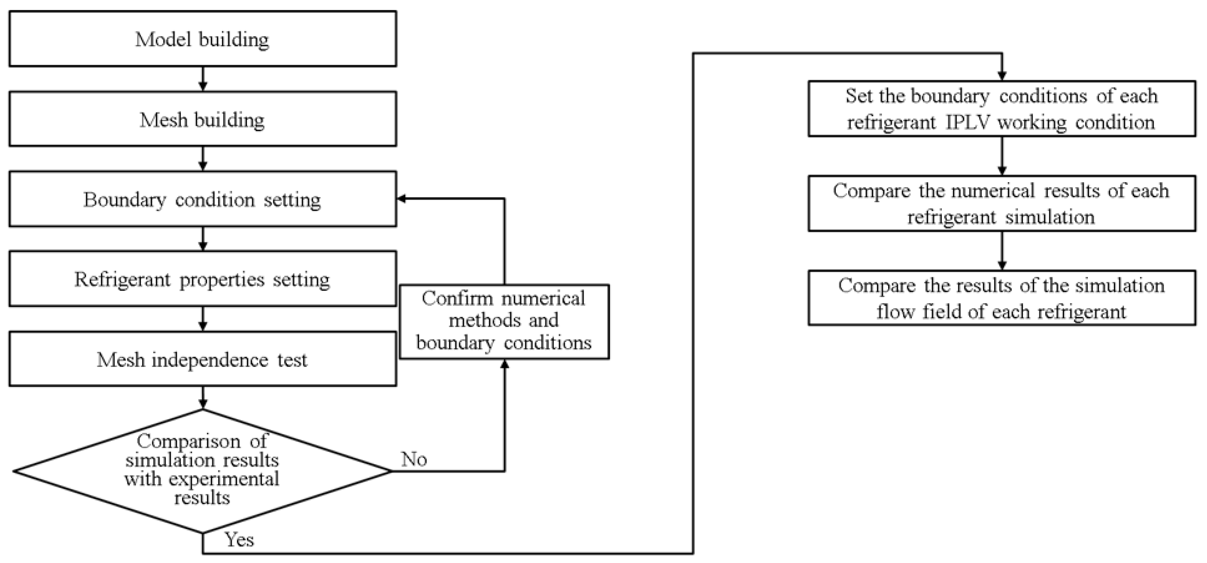
2.1. Research Method

In the present engineering or biotechnological studies, there are many instances wherein computational fluid dynamics (CFD) is used to predict the fluid flow or various reaction phenomena. As the calculator computation capability has been enhanced, the initially time-consuming calculation can be completed within several hours. The fluid behavior governing equation is computed using a numerical method.

The governing equations used in this study include Continuity Equation: Equation (2), Momentum Equation: Equation (3), and Total Energy Equation: Equation (4), expressed as follows.

Continuity Equation [25]

$$\frac{\partial \rho }{\partial t}+\nabla ·\left(\rho U\right)=0$$

(2)

Momentum Equation [25]

$$\frac{\partial \left(\rho U\right)}{\partial t}+\nabla ·\left(\rho U\otimes U\right)=-\nabla p+\nabla ·\tau +S_M$$

(3)

Total Energy Equation [25]

$$\frac{\partial \left(\rho h_{tot}\right)}{\partial t}-\frac{\partial p}{\partial t}+\nabla ·\left(\rho U{h}_{tot}\right)=\nabla ·\left(\lambda \nabla T\right)+\nabla ·\left(U·\tau \right)+U·S_M+S_E$$

(4)

Rutvika Acharya [26] mentioned that the k-epsilon (k-ε) model was a general-purpose turbulence model in terms of turbulence models. The k-omega (k-ω) model had a better computation capability for the boundary layer of the low Reynolds number flow field. The Shear Stress Transport (SST) model was mixed with the k-epsilon (k-ε) and k-omega (k-ω) models. The method was that the k-omega (k-ω) model was started near the wall surface, and the k-epsilon (k-ε) model was started far from the wall surface. According to the R134a refrigerant compressor simulation results (as shown in

Table 4. Comparison of the results from different turbulence models.

Refrigerant	R134a
Rotating Speed(RPM)	17010
Inlet Total Temperature (℃)	6.6
Inlet Total Pressure (kPa)	365.74
Outlet Mass Flow Rate (kg/s)	6.383
Turbulence Model	k-epsilon	k-omega	SST
CPU Time (min)	154	150	163
Total Pressure Ratio	2.42	2.47	2.47
Torque (N·m)	74.47	74.55	74.57
Outlet Total Temperature (℃)	39.08	39.37	39.38
Outlet Total Pressure (kPa)	886.41	901.36	901.77
Isentropic Compression Efficiency (%)	90.56	92.18	92.20

), the calculation time and calculation result error comparison analysis showed that in the same analog network and the same boundary conditions, the k-omega (k-ω) model had the shortest calculation time, and the error in the simulation results did not exceed 2%. Hence, this study selected the k-omega (k-ω) model as the simulation turbulence model.

This study’s numerical simulation analysis software is Ansys integrated software of the U.S. Ansys software firm. It uses drawing software SpaceClaim, meshing software Meshing and TurboGrid, numerical simulation software CFX and post-processing software CFD-Post. All of the said software is integrated with Ansys Workbench for integrated operation. The CFX numerical simulation software can perform simulated computation for rotating fluid machinery, shorten the calculation time and enhance the calculation precision compared to the Fluent numerical simulation software of Ansys.

2.2. Execution Procedure

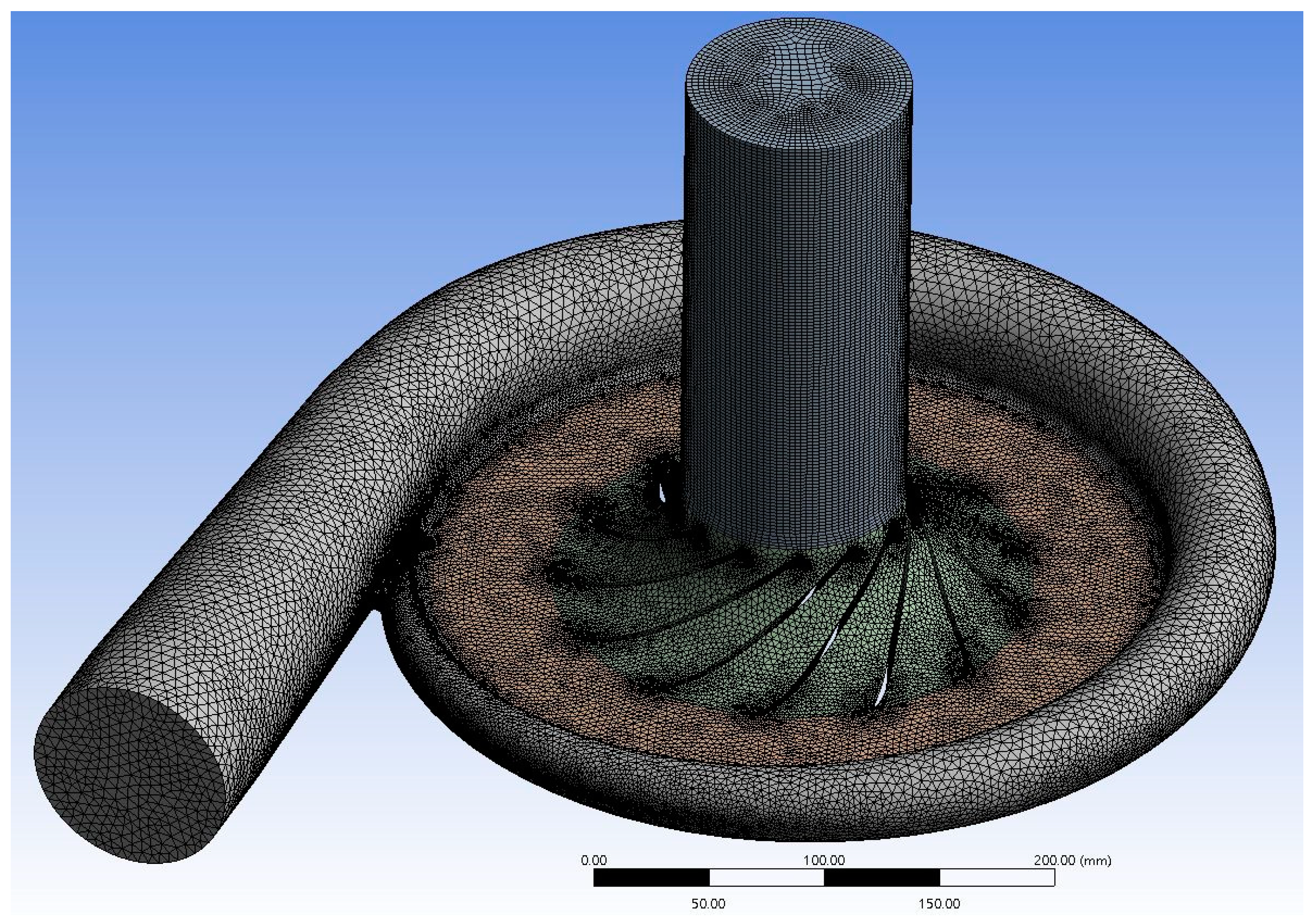
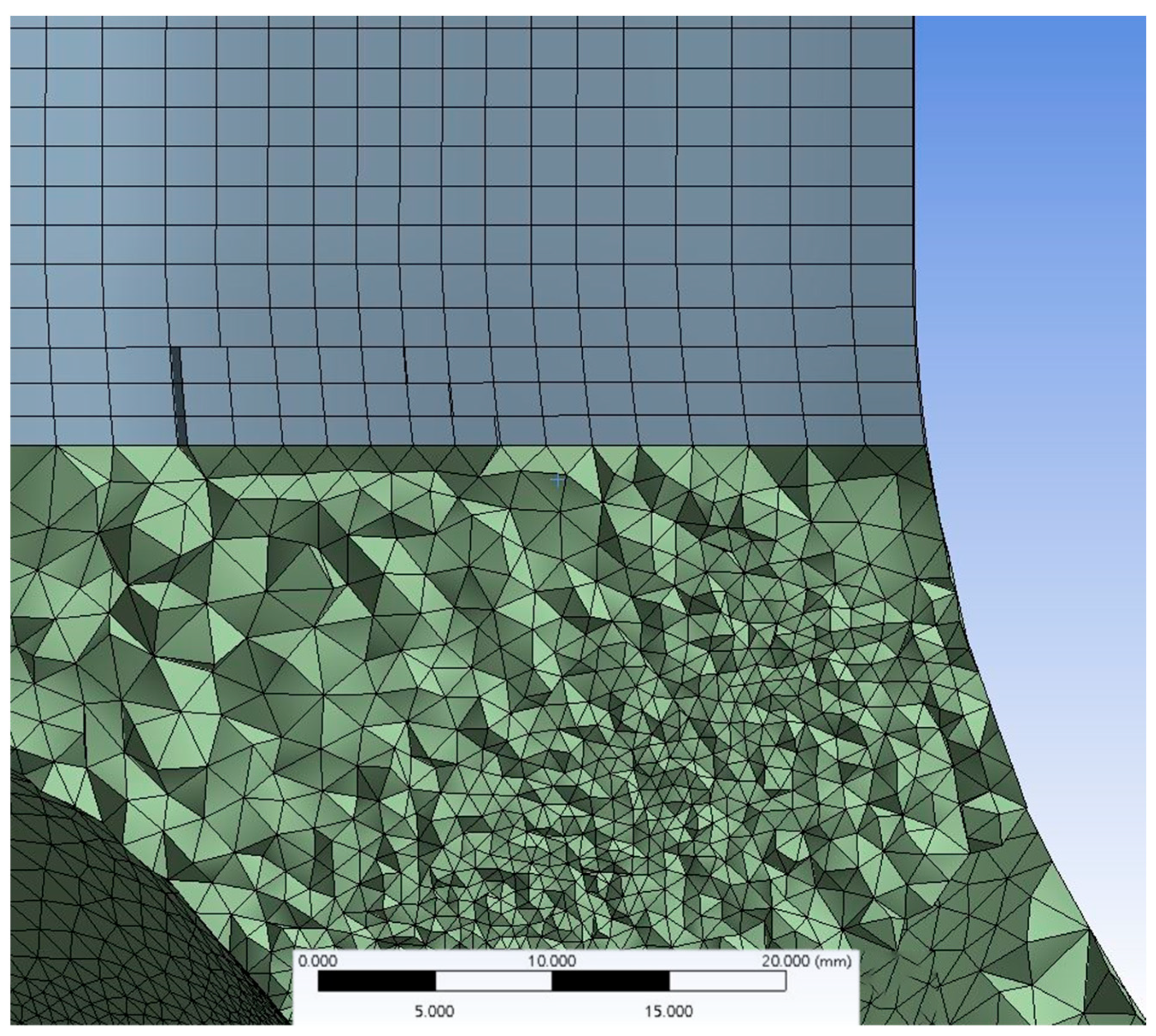
The flowchart of the execution procedure is shown in Figure 4. For numerical flow field simulation, the flow field computational domain must be given first. In this study, the first step is to divide the SolidWorks graphics file drawn by the Industrial Technology Research Institute into three objects the inlet zone, rotor zone, and outlet zone. The file was converted to a.x_t or. step file and drawn in Ansys-DesignModeler or Ansys-SpaceClaim drawing software for a combined building and repairing a model. This is easier for Ansys-Meshing to create the simulation mesh. The simulation mesh number was increased by changing the mesh growth rate. The impeller torque and total pressure ratio were monitored for the mesh independence test to determine the simulation mesh number. Afterward, a numerical simulation was performed for the IPLV refrigerant condition. The simulation result and flow field were discussed to observe whether there was abnormal flow behavior. The characteristic curve and compression ratio and flow field efficiency curves were worked out.

2.2.1. Meshing

Meshing is the process of defining the minimum unit of the numerical simulation computational domain. The mesh size can determine the number of grids and the calculation results resolution. The quality of a mesh can determine the calculation convergence difficulty level and the calculation results precision. The total number of grids can influence the simulation calculation time. To generate a mesh with adequate quality, meeting computer effectiveness and shorter calculation time, the time consumption sometimes exceeds the time for computation. However, for the correctness of the calculation, it is necessary to test the mesh repeatedly. The generated global mesh of the compressor is shown in Figure 5 (left), and the enlarged view of the joint of the mesh is shown in Figure 6 and Figure 7.

2.2.2. Boundary Condition Setting

The boundary conditions and parameters in the IPLV experiment of centrifugal refrigerant compressor include the water inlet temperature, water outlet temperature, and flow of the iced waterside, the water inlet temperature, water outlet temperature, and flow of the cooled waterside, power consumption analysis, and the compressor inlet/outlet pressure. The boundary condition setting method calculates the inlet temperature and pressure of the actual compressor and the mass flow rate of the refrigeration cycle based on these numbers. The calculation results were set as the simulation boundary conditions. The following assumptions were made for numerical simulation:

• Steady-state flow field
• Smooth adiabatic wall surface
• Leakage loss is ignored
• The gravity effect is ignored.

The R134-a magnetic levitation centrifugal refrigerant compressor boundary condition setting parameters of 280 USRT are shown in

Table 5. Description of boundary condition and parameter setting methods.

Name	Setting Conditions and Parameters
Working Fluid	R134a
IPLV Load		100%	75%	50%	25%
Inlet	Total Temperature (°C)	6.6	6.8	7	7
	Total Pressure (kPa)	365.74	368.26	370.80	370.80
Outlet	Mass Flow Rate (kg/s)	100%	70%	44%	22%
Rotating Speed	Rated Speed (rpm)	100%	86%	72%	69%
Turbulence Model	k-omega turbulence model (k-ω)
Discretization Method	Specified Blend Factor (0.5)

. This study performed numerical simulations for R-513A refrigerant in 1000 kW level and 525 kW level operating conditions.

2.2.3. Refrigerant Properties Setting

This study used the built-in SRK (Soave Redlich Kwong) gas Equations (5)–(11) of CFX as the fluid property computed by CFD, including R-134a, R-1234yf, and R-513A refrigerants, expressed as follows [25].

$$p=\frac{RT}{v-b+c}-\frac{a\left(T\right)}{v\left(v+b\right)} p=\mathrm{Pressure} \left(\mathrm{kPa}\right)$$

(5)

$$b=0.08664\frac{R{T}_c}{p_c} T=\mathrm{Temperature} \left(\mathrm{K}\right)$$

(6)

$$a\left(T\right)=a_0{\left(1+n\left(1-\sqrt{\frac{T}{T_C}}\right)\right)}^2 R=\mathrm{Gas}\mathrm{constant}(\mathrm{kJ}/\mathrm{kg} \mathrm{K})$$

(7)

$$a_0=0.42747\frac{R^2{T}_c{}^2}{P_C} v=\mathrm{Specific}\mathrm{Volume}({\mathrm{m}}^3/\mathrm{kg})$$

(8)

$$n=0.480+1.574\omega -0.176{\omega }^2 T_c=\mathrm{Critical} \mathrm{Temperature} \left(\mathrm{K}\right)$$

(9)

$${\left(dp/dv\right)|}_T=0 p_c=\mathrm{Critical} \mathrm{Pressure} \left(\mathrm{kPa}\right)$$

(10)

$$lo{g}_{10}\left(\frac{p_v}{p_c}\right)=\frac{7}{3}\left(1+\omega \right)\left(1-\frac{T_c}{T}\right) \omega =\mathrm{Acentric} \mathrm{Factor}$$

(11)

The heat transfer capacity of refrigerant was calculated from the zero pressure coefficients, expressed as follows (Equations (12) and (13)) [25].

$$\begin{gathered} \frac{C_{\mathrm{p}}^0}{R}=a_1+a_{2}T+a_3{T}^2+a_4{T}^3+a_5{T}^4 \\ R=\mathrm{Gas} \mathrm{constant} (\mathrm{kJ}/\mathrm{kg} \mathrm{K}) \end{gathered}$$

(12)

$$\begin{gathered} C_{\mathrm{p}}^0=\mathrm{Specific} \mathrm{Heat} \mathrm{at} \mathrm{Zero} \mathrm{Pressure} (\mathrm{kJ}/\mathrm{kg} \mathrm{K}) \\ T=\mathrm{Temperature} \left(\mathrm{K}\right) \end{gathered}$$

(13)

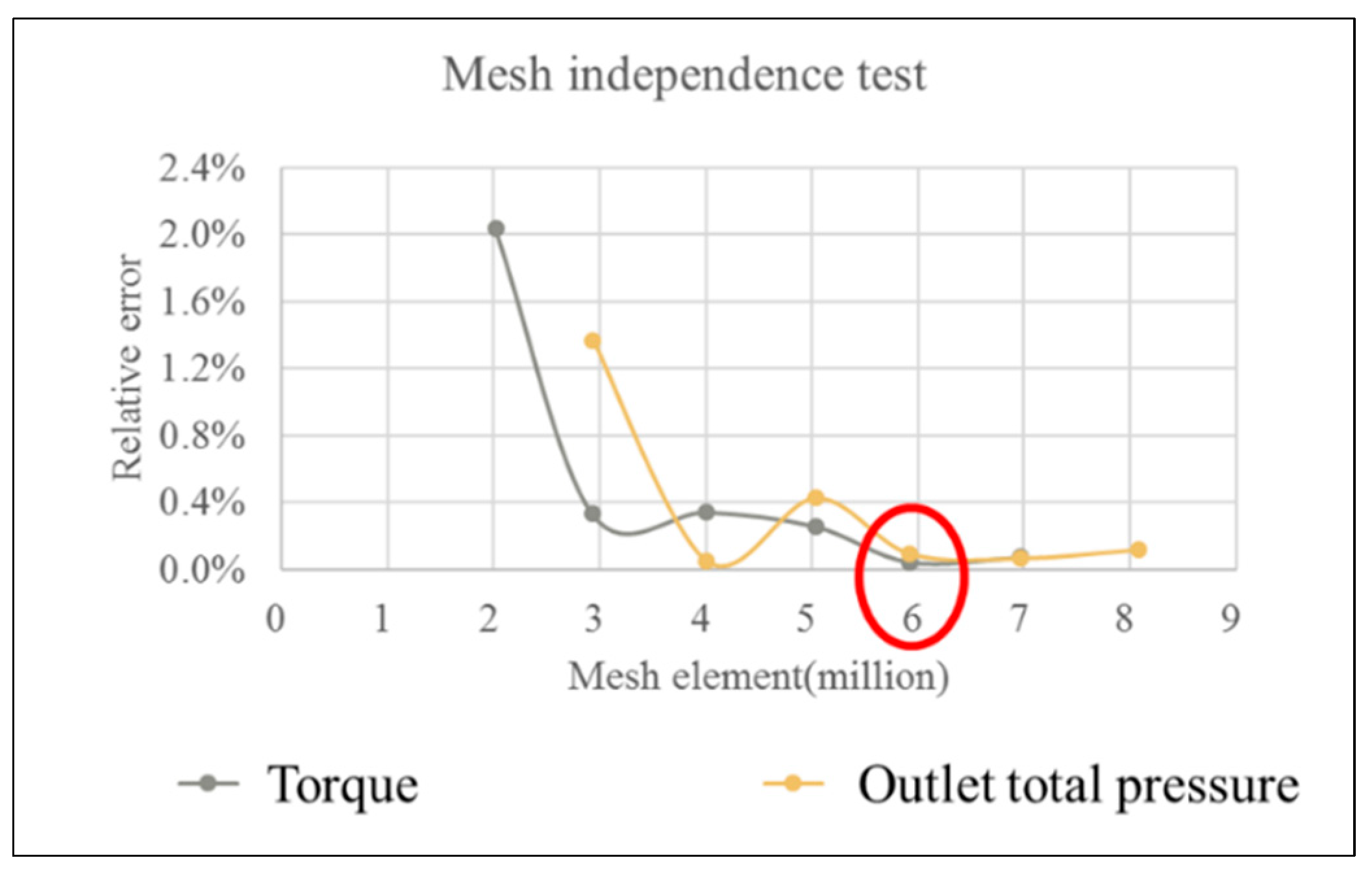
2.2.4. Mesh Independence Test

This study made 2 million mesh to 8 million mesh for the flow element model of 280USRT magnetic levitation centrifugal refrigerant compressor. Every 1 million mesh number was one class interval. There were seven meshes, and the quality of each mesh met the regulation below mesh skewness of 0.95. The computational condition was R-134a refrigerant at full load condition. After the relative impeller torque error and relative outlet total pressure error were compared, 6 million mesh number was selected as the simulation mesh, because the relative error of 6 million mesh number value is the smallest, as shown in red circle on Figure 8. The relative error computing mode (Equation (14)) and mesh independence result are shown in Figure 8:

$$\begin{gathered} \mathrm{Relative} \mathrm{error}=\frac{\left|\mathrm{A}-\mathrm{B}\right|}{\mathrm{A}}\times 100\% \\ \mathrm{A}=\mathrm{After} \mathrm{increasing} \mathrm{the} \mathrm{mesh} \mathrm{elements} \\ \mathrm{B}=\mathrm{Before} \mathrm{increasing} \mathrm{the} \mathrm{mesh} \mathrm{elements} \end{gathered}$$

(14)

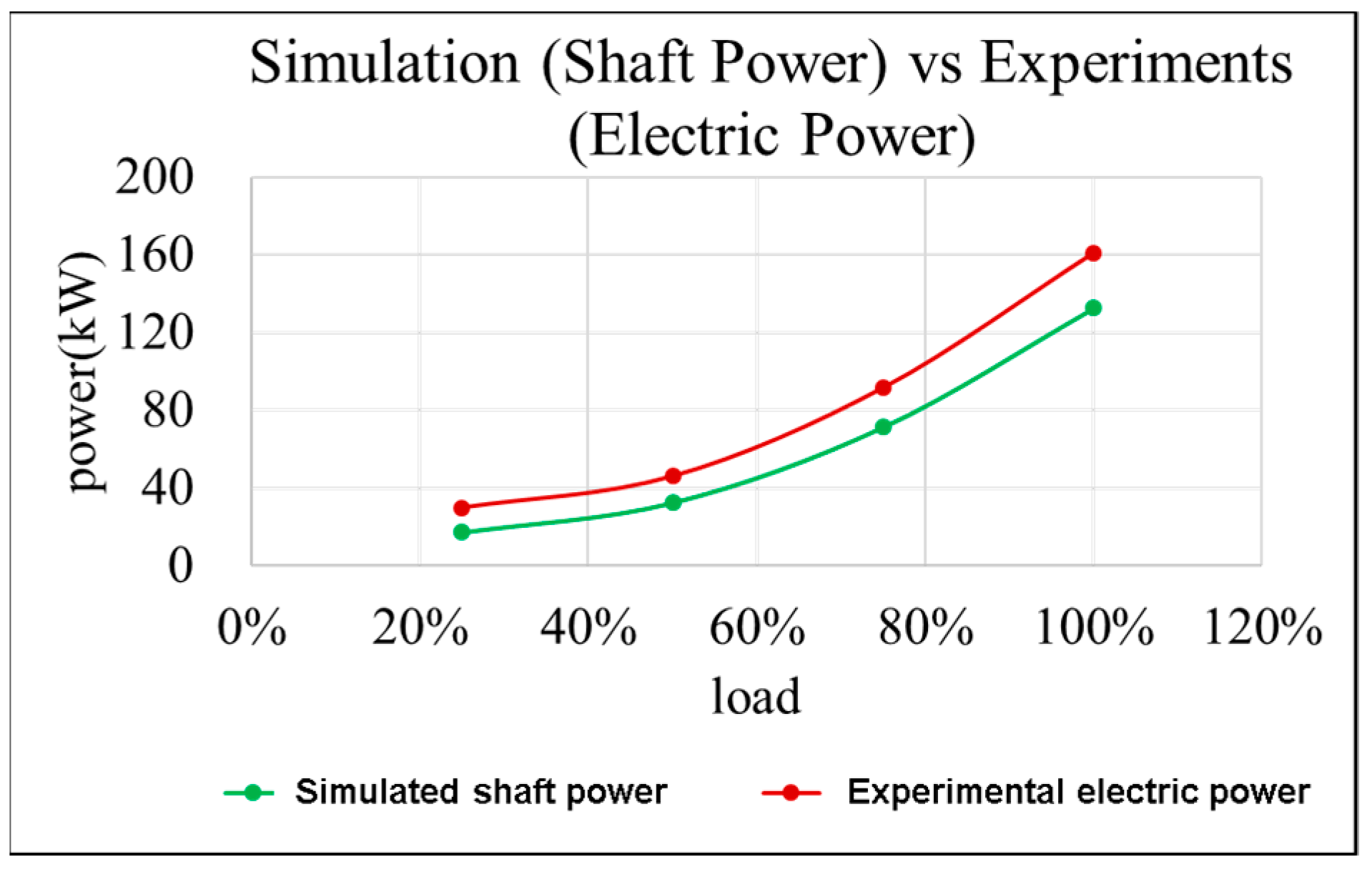
2.2.5. Comparison of Simulation and Experimental Results

The simulation result and experimental result of the IPLV condition are compared based on the overall compression ratio, as shown in

Table 6. Comparison of total pressure ratio between CFD simulation and Experiment.

Load, %	Simulated Total Pressure Ratio	Experimental Total Pressure Ratio	Relative Error
100%	2.47	2.40	2.73%
75%	2.00	1.97	1.48%
50%	1.64	1.61	1.89%
25%	1.60	1.55	3.54%

. Whether the overall compression ratio of various conditions in the simulation result coincides with the experimental result, The maximum difference does not exceed 4%, as shown in Figure 9. the compression ratio computing method and difference computing method (Equations (15) and (16)) are expressed as follows:

$$\mathrm{Total} \mathrm{Pressure} \mathrm{Ratio}=\frac{\mathrm{Outlet} \mathrm{Total} \mathrm{Pressure} \left(\mathrm{kPa}\right)}{\mathrm{Inlet} \mathrm{Total} \mathrm{Pressure} \left(\mathrm{kPa}\right)}$$

(15)

$$\begin{gathered} \mathrm{Relative} \mathrm{error}=\frac{\left|\mathrm{A}-\mathrm{B}\right|}{\mathrm{B}}\times 100\% \\ \mathrm{A}=\mathrm{Experimental} \mathrm{total} \mathrm{pressure} \mathrm{ratio} \\ \mathrm{B}=\mathrm{Simulated} \mathrm{total} \mathrm{pressure} \mathrm{ratio} \end{gathered}$$

(16)

Additionally, the simulated impeller shaft power and experimental compressor power can be compared. Similar power consumption trends are obtained, as shown in Figure 10. The reason for the difference between the two values is that the experimental compressor electric power contains other losses, such as: inverter loss, expressed as follows.

3. Results and Discussion

3.1. Refrigerant Replacement Simulation Analysis—Equation Description

(1)

Total Pressure Ratio

$$\begin{gathered} \mathrm{Total} \mathrm{Pressure} \mathrm{Ratio}=\frac{P_{tot,out}}{P_{tot,in}} \\ {P}_{tot,in} =\mathrm{Inlet} \mathrm{Total} \mathrm{Pressure} \left(\mathrm{kPa}\right) \\ {P}_{tot,out}=\mathrm{Outlet} \mathrm{Total} \mathrm{Pressure} \left(\mathrm{kPa}\right) \end{gathered}$$

(17)

(2)

Isentropic Efficiency

$$\begin{gathered} \mathrm{Isentropic} \mathrm{Efficiency}=\frac{h_{tot,s,out}-h_{tot,in}}{h_{tot,out}-h_{tot,in}} \\ {h}_{tot,in}=\mathrm{Inlet} \mathrm{Total} \mathrm{Enthlpy} (\mathrm{kJ}/\mathrm{kg}) \\ {h}_{tot,out}=\mathrm{Outlet} \mathrm{Total} \mathrm{Enthlpy} (\mathrm{kJ}/\mathrm{kg}) \\ {h}_{tot,s,out}=\mathrm{Outlet} (\mathrm{kJ}/\mathrm{kg}) \end{gathered}$$

(18)

(3)

Shaft Power

Shaft Power = Torque × ω
Torque = Torque of Impeller (N)
ω = Rotating Speed of Impeller (rad/s)

(19)

(4)

COP (Coefficient of Performance)

Coefficient of Performance = Q_e/(Shaft Power)
Q_e = Refrigeration capacity (kW)     Shaft Power = Shaft Power (kW)

(20)

(5)

IPLV (Integrated Part Load Value)

IPLV = 0.01A + 0.42B + 0.45C + 0.12D
A = COP at 100% load     B = COP at 75% load
C = COP at 50% load     D = COP at 25% load

(21)

3.2. Refrigerant Replacement Simulation Analysis—Numerical Simulation Result

3.2.1. Total Pressure Ratio Comparison

In the case of the 25% to 75% load, the total pressure ratio of R-1234yf refrigerant was the highest. The total pressure ratio of R-513A took second place. The total pressure ratio of R-134a was the lowest. In the case of full load, the total pressure ratios of R-1234yf and R-513A decreased slightly. This is because the alternative refrigerant had a smaller enthalpy difference, the flow was increased to the chokepoint, and the total pressure ratio was reduced, as shown in Figure 11.

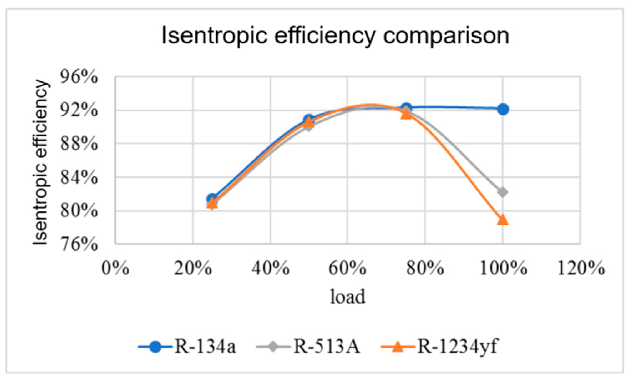
3.2.2. Isentropic Efficiency Comparison

In the case of the 25% to 75% load, three refrigerants had similar isentropic efficiencies compared to the 50% to 75% load. The isentropic efficiency of 25% load was lower. It might have been caused by flow loss in the flow field. In the case of full load, the isentropic efficiency of various refrigerants decreased as the mass flow rate increased, as shown in Figure 12.

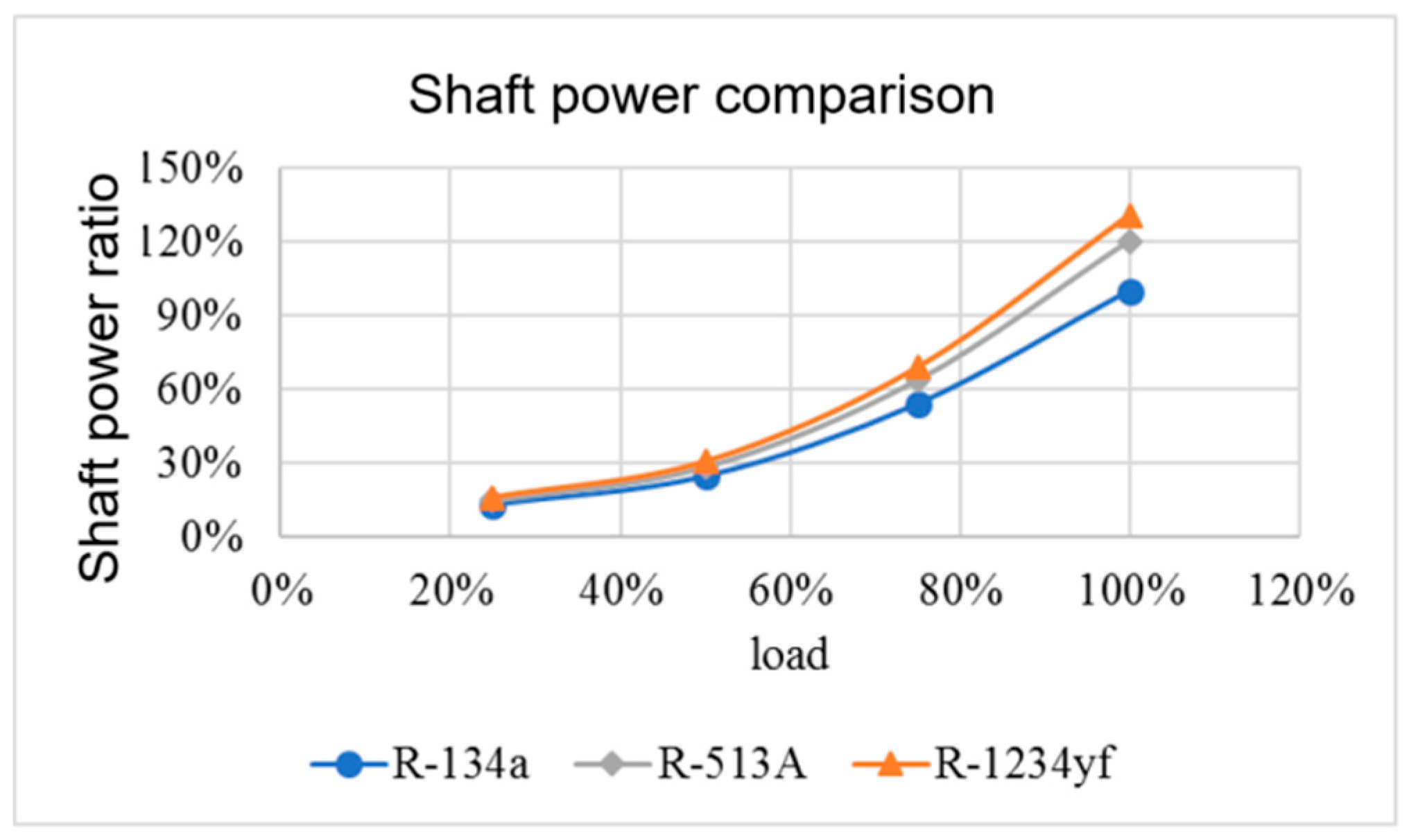
3.2.3. Shaft Power Comparison

The enthalpy difference decreased in the alternative refrigerant evaporation process to achieve the same refrigerating capacity. The required mass flow rate increased, and the impeller shaft power for pushing the refrigerant also increased. As the rotation speed increased, the phenomenon was more apparent, as shown in Figure 13.

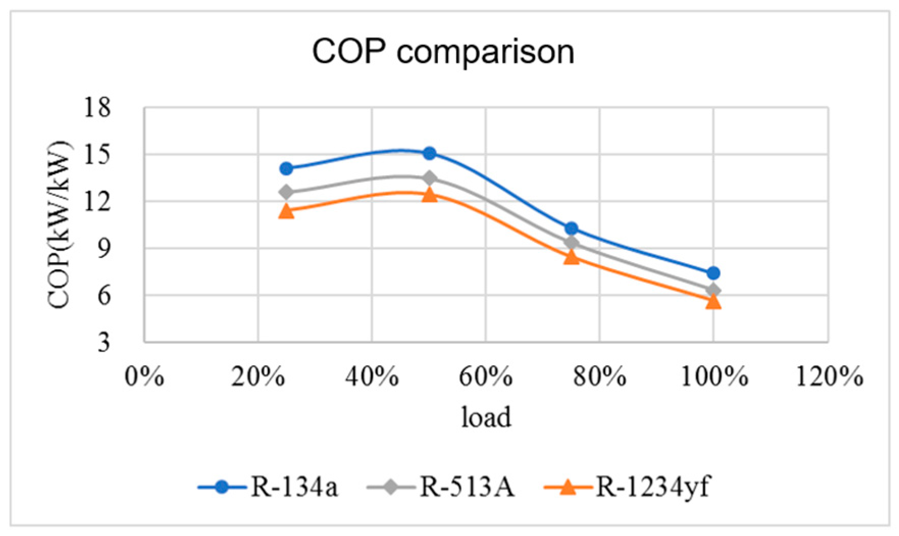
3.2.4. COP Comparison

The R-134a refrigerant had the highest COP in various conditions. The R-1234yf refrigerant had the lowest COP, and the R-513A was intermediate among the other two refrigerants, as shown in Figure 14.

3.2.5. IPLV Comparison

After IPLV weighted calculation, compared to singly comparing full load COP, the IPLV values of various refrigerants are closer, as shown in Figure 15.

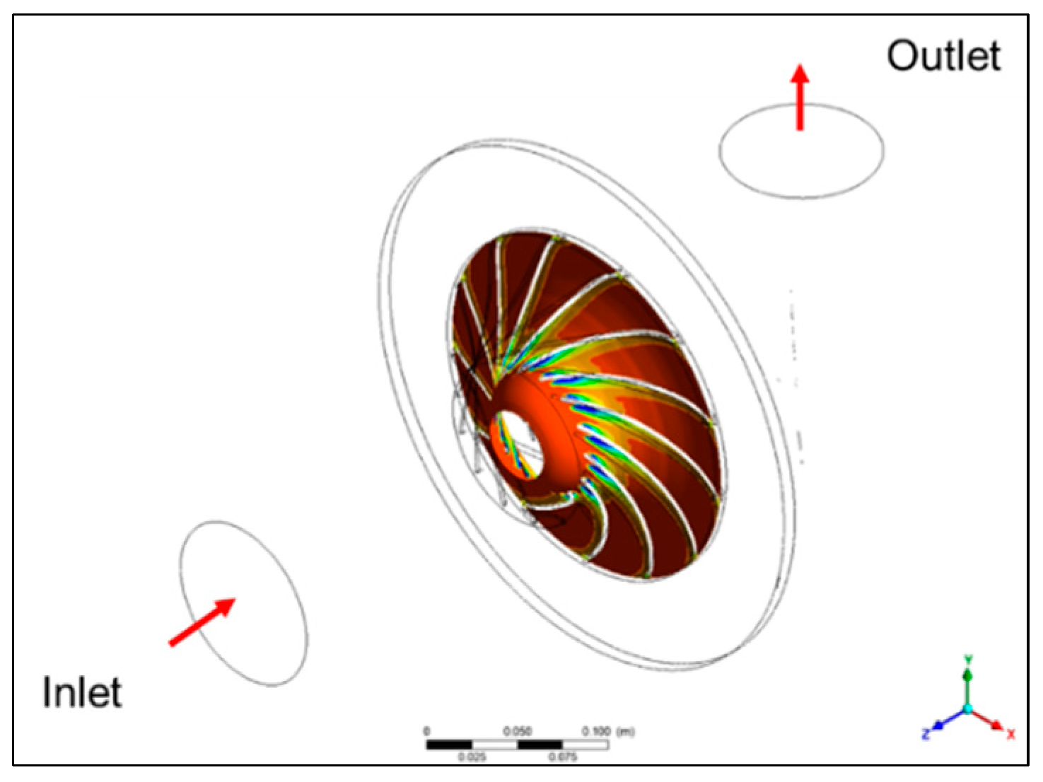
3.3. Refrigerant Replacement Simulation Analysis—Flow Field Simulation Result

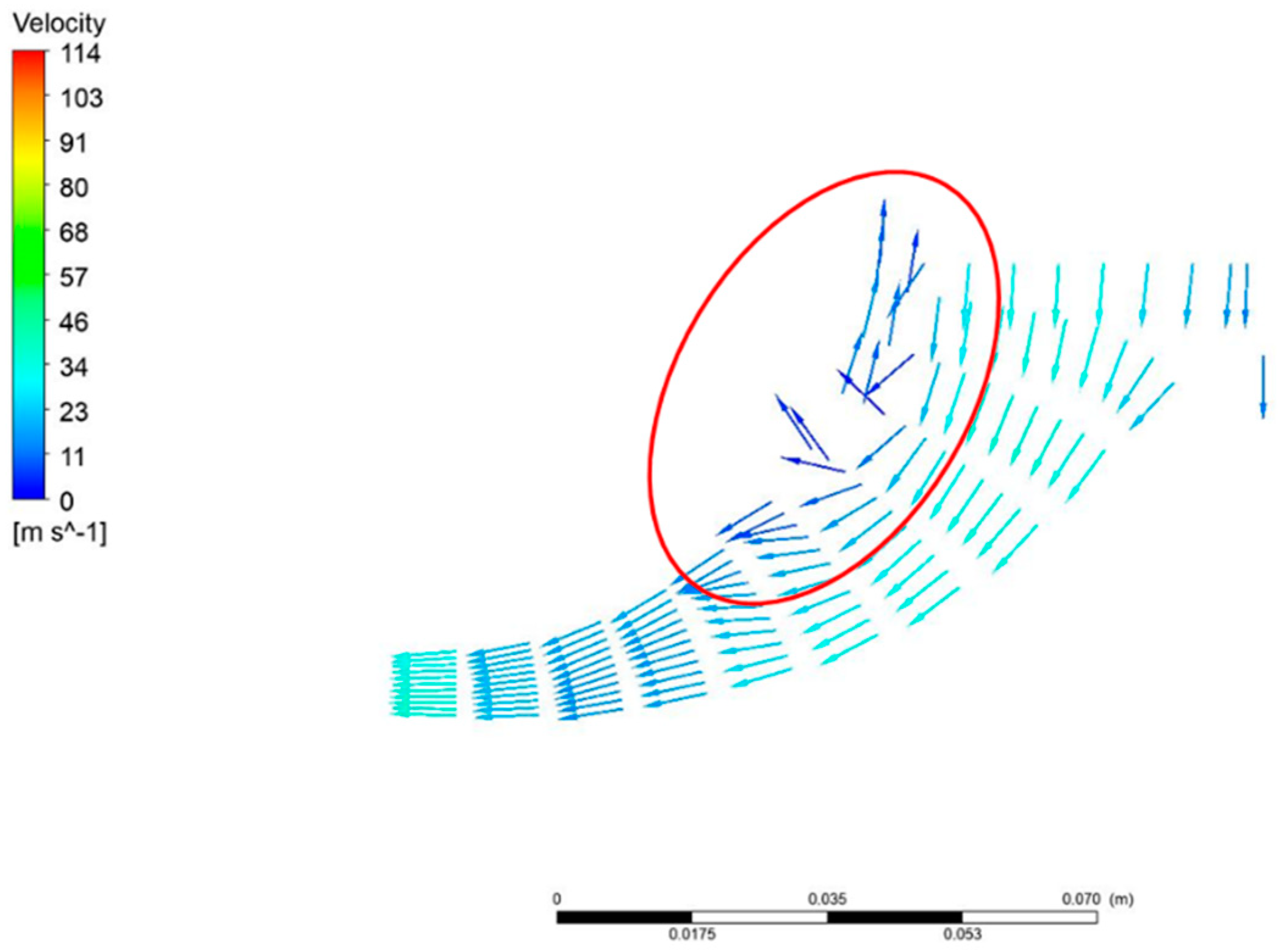
3.3.1. Inter-Blade Flow Field Simulation Result

The schematic diagram of the inter-blade flow field is given below. The flow field is a profile calculation analysis of a proportional spacing between the shroud and hub of the impeller. The Mach-number distribution of the flow field near the shroud among the blades was analyzed, as shown in Figure 16.

When the compressor is operating at the choke point, because of the larger mass flow rate, the fluid velocity inside the compressor continues to increase until it reaches the speed of sound (Mach Number 1) or resonance at the blade throat and no more flow can pass through the compressor, causing a choking effect. This phenomenon is the reason for the drop in pressure ratio and isentropic efficiency in the full load condition of R-1234yf refrigerant and R-513A refrigerant, as shown in Figure 17.

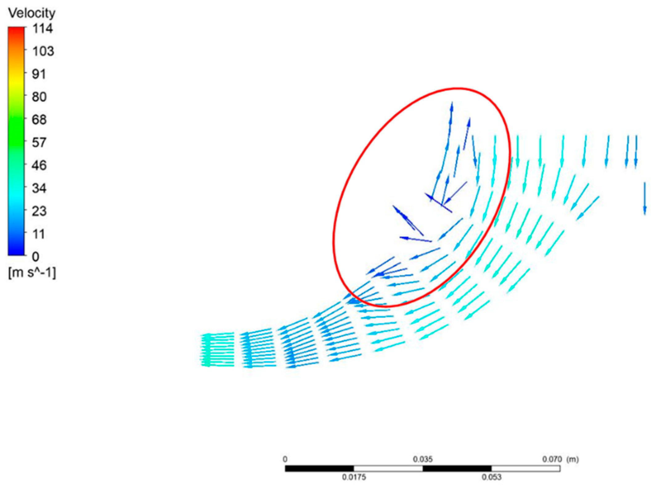
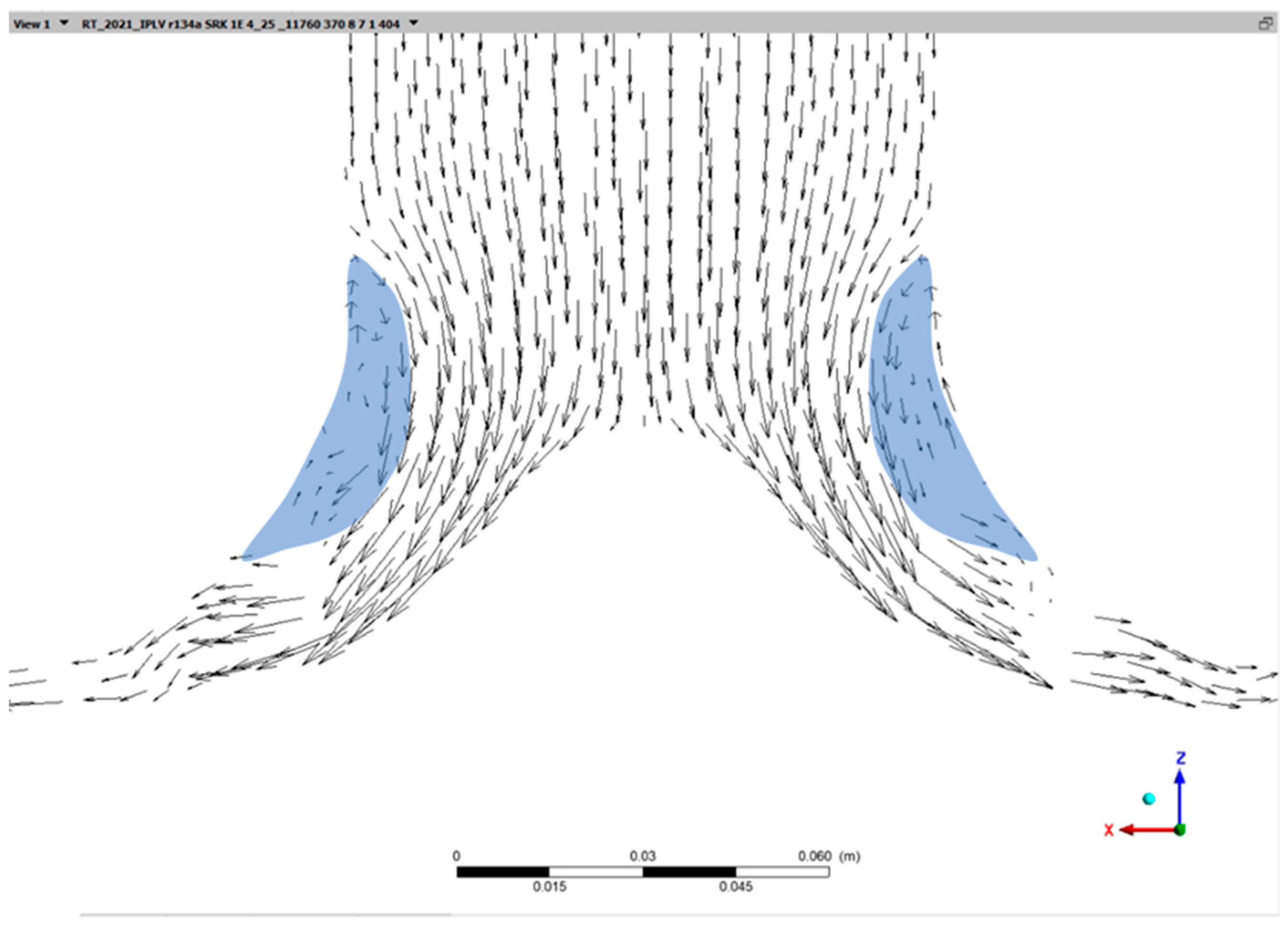
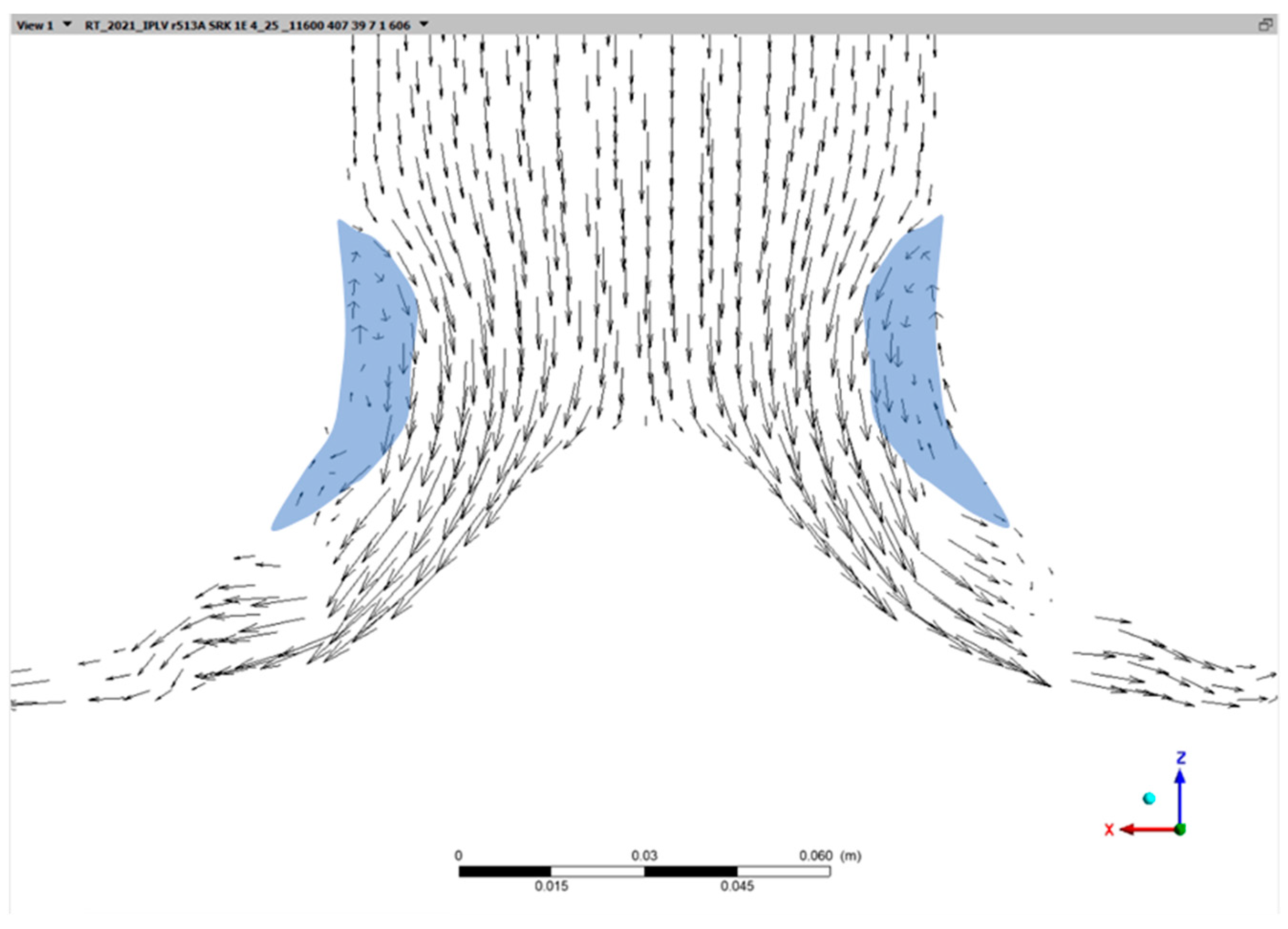
3.3.2. Flow Field on Meridian Plane Analysis Result

The meridian plane flow field sampling location on the impeller is on the ZX plane based on the +X direction. The refrigerant fluid flows through the red mark at the inlet and flows out through the blue mark at the outlet. The yellow mark is the shroud, and the purple mark is the hub. The impeller rotation direction is z-axis, as shown in Figure 18.

The velocity vectors at the impeller eye of various refrigerants in 25% load condition are shown in the following diagrams. It is observed that there are different colors near the shroud in the impeller’s eye. There are obvious swirls, and the reason for the swirls is that the load condition is close to the surge point. The swirls significantly influence the overall compressor efficiency, as shown in Figure 19, Figure 20, Figure 21, Figure 22, Figure 23 and Figure 24. Refs. [13,15] suggest that when the compressor condition is close to the surge point, there is back-flow at the impeller, and the swirls also significantly affects the efficiency of the compressor. This phenomenon is similar to the simulation in this study.

In the future, in order to find the best replacement refrigerant, the simulation results of different HFO refrigerants will be added for comparison, and the simulation results of different refrigerants will be verified by experiments, including R-513A refrigerant IPLV experiment and R-1234yf refrigerant IPLV experiment, and add compressors Transient simulation results to analyze the effect of the compressor under rotating stall to understand the efficiency and cost-effectiveness of replacing refrigerant.

4. Discussion and Conclusions

4.1. According to the Numerical Analysis Result of Various Refrigerants in IPLV Condition

(a)

In full load condition of R-1234yf and R-513A refrigerant compared to R-134a refrigerant, the isentropic efficiency of R-1234yf refrigerant is reduced by 13.21%, and the isentropic efficiency of R-513A refrigerant is reduced by 9.97%.

(b)

The first cause for the decrease in isentropic efficiency under full load is excessive refrigerant flow. The compressor operating point is located at or near the choke point.

(c)

In 75%, 50%, and 25% part-load conditions, the refrigerants have very close isentropic efficiencies. The COP is higher than that in full load conditions. Therefore, the IPLV difference of various refrigerants is smaller than the full load COP difference.

(d)

In IPLV conditions, the total pressure ratio of R-1234yf is higher than R-134a refrigerant by 2.1%~8.3%. The total pressure ratio of R-513A is higher than R-134a refrigerant by about 2.4% under 75%~25% load and lower than R-134a refrigerant by 2.2% under full load.

(e)

R-1234yf and R-513A refrigerants have smaller enthalpy differences in terms of shaft power. A higher refrigerant flow is required so that the shaft work is a little higher than R-134a refrigerant by 31%~23% and 20%~15%.

(f)

In the 25% load condition, various refrigerants have worse isentropic efficiency. The first cause is the swirls near the shroud at the impeller’s eye, the phenomenon is similar to the compressor flow field pattern when it is close to the Surge Point.

4.2. Conclusions

According to the above results, the impeller of the original R134a design is more suitable for the design with a high load of more than 60%. After replacing the R513A or R1234yf, the thermophysical properties including its specific volume and enthalpy are different, and the flow field is more affected when the flow rate is large and the load is high. Obviously, this study shows that direct refrigerant replacement under high load affects the performance more obviously.

References

1. UNEP. Amendment to the Montreal Protocol on Substances That Deplete the Ozone Layer, Kigali, no. 1522 UNTS 3; 26 ILM 1550; UNEP: Nairobi, Kenya, 2016. [Google Scholar]
2. Park, J.H.; Shin, Y.; Chung, J.T. Performance Prediction of Centrifugal Compressor for Drop-In Testing Using Low Global Warming Potential Alternative Refrigerants and Performance Test Codes. Energies 2017, 10, 2043. [Google Scholar] [CrossRef] [Green Version]
3. ASHRAE 34-2019; Designation and Safety Classification of Refrigerants. ASHRAE: Peachtree Corners, GA, USA, 2019; Volume 2019, pp. 1–52. Available online: www.ashrae.org (accessed on 1 May 2022).
4. Lemmon, E.; Huber, M.; McLinden, M. NIST Standard Reference Database 23: Reference Fluid Thermodynamic and Transport Properties-REFPROP, Version 9.1; NIST Standard Reference Data Series (NIST NSRDS); National Institute of Standards and Technology: Gaithersburg, MD, USA, 2013. Available online: https://tsapps.nist.gov/publication/get_pdf.cfm?pub_id=912382 (accessed on 1 May 2022).
5. Hodnebrog, Ø.; Etminan, M.; Fuglestvedt, J.S.; Marston, G.; Myhre, G.; Nielsen, C.J.; Shine, K.P.; Wallington, T.J. Global warming potentials and radiative efficiencies of halocarbons and related compounds: A comprehensive review. Rev. Geophys. 2013, 51, 300–378. [Google Scholar] [CrossRef] [Green Version]
6. Bell, I.H.; Domanski, P.A.; McLinden, M.O.; Linteris, G.T. The hunt for nonflammable refrigerant blends to replace R-134a. Int. J. Refrig. 2019, 104, 484–495. [Google Scholar] [CrossRef] [PubMed]
7. AHRI 550/590; Standard for Performance Rating of Water-Chilling and Heat Pump Water-Heating Packages Using the Vapor Compression Cycle. AHRI: Arlington, VA, USA, 2011; Volume 590, p. 74.
8. Ghenaiet, A.; Khalfallah, S. Assessment of some stall-onset criteria for centrifugal compressors. Aerosp. Sci. Technol. 2019, 88, 193–207. [Google Scholar] [CrossRef]
9. Velásquez, E.I.G. Determination of a suitable set of loss models for centrifugal compressor performance prediction. Chin. J. Aeronaut. 2017, 30, 1644–1650. [Google Scholar] [CrossRef]
10. Zhang, C.; Dong, X.; Liu, X.; Sun, Z.; Wu, S.; Gao, Q.; Tan, C. A method to select loss correlations for centrifugal compressor performance prediction. Aerosp. Sci. Technol. 2019, 93, 1–15. [Google Scholar] [CrossRef]
11. Zhao, D.; Hua, Z.; Dou, M.; Huangfu, Y. Control oriented modeling and analysis of centrifugal compressor working characteristic at variable altitude. Aerosp. Sci. Technol. 2018, 72, 174–182. [Google Scholar] [CrossRef]
12. Kim, C.; Son, C. Comparative Study on Steady and Unsteady Flow in a Centrifugal Compressor Stage. Int. J. Aerosp. Eng. 2019, 2019, 1–12. [Google Scholar] [CrossRef] [Green Version]
13. Zhang, H.; Yang, C.; Shi, X.; Yang, C.; Chen, J. Two stall stages in a centrifugal compressor with a vaneless diffuser. Aerosp. Sci. Technol. 2021, 110, 106496. [Google Scholar] [CrossRef]
14. Tiwari, R.; Bordoloi, D.; Dewangan, A. Blockage and cavitation detection in centrifugal pumps from dynamic pressure signal using deep learning algorithm. Meas. J. Int. Meas. Confed. 2021, 173, 108676. [Google Scholar] [CrossRef]
15. Semlitsch, B.; Mihaescu, M. Flow phenomena leading to surge in a centrifugal compressor. Energy 2016, 103, 572–587. [Google Scholar] [CrossRef]
16. Galindo, J.; Gil, A.; Navarro, R.; Tarí, D. Analysis of the impact of the geometry on the performance of an automotive centrifugal compressor using CFD simulations. Appl. Therm. Eng. 2019, 148, 1324–1333. [Google Scholar] [CrossRef]
17. Sun, J.; Li, W.; Cui, B. Energy and exergy analyses of R513a as a R134a drop-in replacement in a vapor compression refrigeration system. Int. J. Refrig. 2020, 112, 348–356. [Google Scholar] [CrossRef]
18. Yang, M.; Zhang, H.; Meng, Z.; Qin, Y. Experimental study on R1234yf/R134a mixture (R513A) as R134a replacement in a domestic refrigerator. Appl. Therm. Eng. 2019, 146, 540–547. [Google Scholar] [CrossRef]
19. Mota-Babiloni, A.; Belman-Flores, J.M.; Makhnatch, P.; Navarro-Esbrí, J.; Barroso-Maldonado, J.M. Experimental exergy analysis of R513A to replace R134a in a small capacity refrigeration system. Energy 2018, 162, 99–110. [Google Scholar] [CrossRef]
20. Velasco, F.; Illán-Gómez, F.; García-Cascales, J. Energy efficiency evaluation of the use of R513A as a drop-in replacement for R134a in a water chiller with a minichannel condenser for air-conditioning applications. Appl. Therm. Eng. 2021, 182, 115915. [Google Scholar] [CrossRef]
21. Al-Sayyab, A.K.S.; Mota-Babiloni, A.; Navarro-Esbrí, J. Novel compound waste heat-solar driven ejector-compression heat pump for simultaneous cooling and heating using environmentally friendly refrigerants. Energy Convers. Manag. 2021, 228, 113703. [Google Scholar] [CrossRef]
22. Pérez-García, V.; Mota-Babiloni, A.; Navarro-Esbrí, J. Influence of operational modes of the internal heat exchanger in an experimental installation using R-450A and R-513A as replacement alternatives for R-134a. Energy 2019, 189, 116348. [Google Scholar] [CrossRef]
23. Wang, C.-C. An overview for the heat transfer performance of HFO-1234yf. Renew. Sustain. Energy Rev. 2013, 19, 444–453. [Google Scholar] [CrossRef]
24. Janković, Z.; Atienza, J.S.; Suárez, J.A.M. Thermodynamic and heat transfer analyses for R1234yf and R1234ze(E) as drop-in replacements for R134a in a small power refrigerating system. Appl. Therm. Eng. 2015, 80, 42–54. [Google Scholar] [CrossRef]
25. ANSYS. ANSYS CFX-Solver Theory Guide. Release 14.0; ANSYS: Canonsburg, PA, USA, 2011; Volume 15317, pp. 724–746. Available online: http://www1.ansys.com/customer/content/documentation/140/cfx_thry.pdf (accessed on 1 May 2022).
26. Acharya, R. Investigation of Differences in Ansys Solvers CFX and Fluent; KTH Royal Institute of Technology: Stockholm, Sweden, 2016. [Google Scholar]
Figure 1. P-h thermodynamic cycle diagrams of single-stage (left) and two-stage (right) centrifugal compressors.
Processes 10 00928 g001
Figure 2. Exploded diagram of an impeller.
Processes 10 00928 g002
Figure 3. Mollier diagram of different refrigerants under the same evaporation and condensation conditions.
Processes 10 00928 g003
Figure 4. Flow field simulation analysis structure diagram.
Processes 10 00928 g004
Figure 5. Global diagrams of compressor model meshes.
Processes 10 00928 g005
Figure 6. Joint of inlet tube and impeller of mesh.
Processes 10 00928 g006
Figure 7. Joint of impeller and diffuser of mesh.
Processes 10 00928 g007
Figure 8. Schematic diagram of mesh independence test.
Processes 10 00928 g008
Figure 9. Comparison diagram of total pressure ratios of simulation and experiment.
Processes 10 00928 g009
Figure 10. Comparison chart of simulated shaft power and experimental electric power.
Processes 10 00928 g010
Figure 11. Comparison diagram of total pressure ratio of refrigerants.
Processes 10 00928 g011
Figure 12. Comparison diagram of isentropic efficiency of refrigerants.
Processes 10 00928 g012
Figure 13. Comparison diagram of shaft power of refrigerants.
Processes 10 00928 g013
Figure 14. Comparison diagram of COP of refrigerants.
Processes 10 00928 g014
Figure 15. Comparison diagram of full load COP and IPLV of refrigerants.
Processes 10 00928 g015
Figure 16. Schematic diagram of the inter-blade flow field of a refrigerant compressor.
Processes 10 00928 g016
Figure 17. Numerical dispersion of Mach number of the inter-blade flow field of refrigerants.
Processes 10 00928 g017
Figure 18. Schematic diagram of meridian plane flow field position.
Processes 10 00928 g018
Figure 19. Compressor meridional velocity vector diagram of R-134a refrigerants under 25% load.
Processes 10 00928 g019
Figure 20. Compressor meridional velocity vector diagram of R-1234yf refrigerants under 25% load.
Processes 10 00928 g020
Figure 21. Compressor meridional velocity vector diagram of R-513A refrigerants under 25% load.
Processes 10 00928 g021
Figure 22. Compressor impeller velocity vector diagram of R-134a refrigerants under 25% load.
Processes 10 00928 g022
Figure 23. Compressor impeller velocity vector diagram of R-1234yf refrigerants under 25% load.
Processes 10 00928 g023
Figure 24. Compressor impeller velocity vector diagram of R-513A refrigerants under 25% load.
Processes 10 00928 g024