Article

A Supplier Selection Model Using Alternative Ranking Process by Alternatives’ Stability Scores and the Grey Equilibrium Product

1
Geneva School of Economics and Management, University of Geneva, 1211 Geneva, Switzerland
2
School of Computer Science and Informatics, De Montfort University, The Gateway, Leicester LE1 9BH, UK
*
Author to whom correspondence should be addressed.
Processes 2022, 10(5), 917; https://doi.org/10.3390/pr10050917
Submission received: 18 February 2022 / Revised: 25 April 2022 / Accepted: 30 April 2022 / Published: 6 May 2022

Abstract

:
Supply chain management begins with supplier evaluation and selection. The supplier selection deals with various criteria with different contexts which makes it a complex multi-criteria decision-making (MCDM) method. In this paper, a novel MCDM method, called the alternative ranking process by alternatives’ stability scores (ARPASS), is proposed to solve supplier selection problems. ARPASS considers each alternative as a system that is constructed on integrated components. To perform properly, a system requires high integrity and stability. ARPASS utilizes the stability of alternatives as an effective element for ranking the alternatives. The ARPASS is developed in two forms, ARPASS and ARPASS*. The new method utilizes standard deviations and Shannon’s entropy to compute the alternatives’ stabilities. In this paper, in addition to the new MCDM methods, a new method called the grey equilibrium product (GEP) is introduced to convert grey linguistic variables into crisp values, using decision makers’ subjective perceptions and judgments. To highlight and validate the novel methods’ performance, they are applied to two sustainable supplier selection problems. For evaluation of the reliability of ARPASS and ARPASS*, their results were compared with the results of the popular MCDM methods. We compared the methods in terms of calculation time, simplicity, transparency, and information type.

1. Introduction

Firms require an efficient supply chain management order to integrate all activities involved in the supply chain, from ordering and raw materials procurement to products production process, and the distribution to markets [1]. The supply chain is constructed on several activities including the procurement of the materials, processing them into intermediate goods and final products, delivering the product to customers, which encompasses all links from suppliers to customers [2]. The very first step of supply chain management is supplier evaluation and selection [3]. Supplier evaluation is a non-stop process of the suppliers’ assessment which includes a qualified verification process [4]. The mentioned process’ goal is to find a supplier who can provide the finest product or service for the least cost which eventually results in a high level of profit and quality [5].
The selection of the best supplier could be addressed as one of the key factors that contributes to the operational success of firms, yet this process consumes time and resources [6]; therefore, the process is vital to decrease the cost of the supply chain. In general, supplier evaluation/selection is a complex multi-criterion decision-making (MCDM) problem which embraces a number of suppliers and various criteria. MCDM methods have been categorized under two categories: discrete problems which are handled by multi-attribute decision-making (MADM) or generally MCDM and continuous problems handled by multi-objective decision-making (MODM) techniques. MADM and MCDM problems are constructed on ( n ) numbers of evaluation criteria and ( m ) numbers of alternative decision possibilities [7], where the criteria are stochastic or random [8].
An MCDM problem is generally illustrated as a decision matrix form. A typical decision matrix has been illustrated in (Equation (1)), where A i = A 1 , A 2 ,   , A m and C j = C 1 , C 2 , , C n are sets of feasible alternatives and decision-making criteria, respectively. In addition, ( x m n ) is the score of m th ( A ) against the n th ( C ).
X = x 11 x 12 x 1 n x 21 x 22 x 2 n x m 1 x m 2 x m n
Throughout the years, several MCDM techniques have been developed which offer their solutions by making using of different algorithms and philosophies such as RBOP (ranking based on optimal points multi-criteria decision-making method) [9], SWARA (step-wise weight assessment ratio analysis) [10], “subjective weighting method using continuous interval scale” [11], SIR (the superiority and inferiority ranking) method [12], IMP (multi-attribute evaluation using imprecise weight estimates) method [13], and BWM (best–worst method) introduced by [14]. The most popular MCDM methods that are widely applied to solve decision-making problems are as the following list: TOPSIS (The Technique for Order of Preference by Similarity to Ideal Solution) introduced by [15]; AHP (the analytic hierarchy process) which was first introduced by [16,17]; ANP (analytical network process) by [18]; SAW (simple additive weighted) developed by [19]; DEA (Data Envelopment Analysis) proposed by [20]; VIKOR (Vise Kriterijumska Optimizacija I Kompromisno Resenje) [21,22]; DEMATEL (decision-making trial and evaluation laboratory) [23], preference ranking organization method for enrichment evaluations “PROMETHEE” [24], and ELECTRE (ELimination Et Choix Traduisant la REalité or ELimination and Choice expressing reality) which was first introduced by [25,26,27,28]. The comparison of MCDM methods can be found in [29,30,31,32,33,34,35,36]. In general, MCDM methods can be categorized into two categories of MCDM weighting methods and MCDM ranking methods in accordance with their performance in evaluation of the alternatives or criteria. The MCDM weighting methods are generally categorized as objective methods, e.g., Shannon’s entropy, see [37], and subjective methods, e.g., AHP, where the objective method relies on the decision makers’ opinions and perception, while the objective methods extract the weights from the decision matrix. Several categorizations of the MCDM ranking methods exist, see [7], yet in general they could be categorized into four categories including the outranking method (ELECTRE, PROMETHEE), compromise ranking (GRA), distance-based (VIKOR, TOPSIS), and pairwise comparison (AHP, ANP).
The mentioned taxonomies generate the outputs through different processes. The distance-based method compares alternatives with at least one ideal alternative that does not have an independent existence and is extracted from the decision matrix itself; TOPSIS and VIKOR are two popular examples of this category. Rashidi and Cullinane [38] utilized fuzzy DEA and fuzzy TOPSIS in their work for a logistics service providers case in Sweden. Yu et al. [39] employed group decision making and extended TOPSIS under interval-valued Pythagorean fuzzy environment. VIKOR has been applied to the research of Karami et al. [40] and Zhang and Yang et al. [41] to solve sustainable supplier selection problems. Pairwise comparison is an appropriate tool to measure preference values of limited alternatives with regard to the decision-making problem’s criteria [42]. AHP is the most popular method of this category that has evolved in different extensions through past four decades, yet it is generally applied in combination with other MCDM methods. The examples of recent application of AHP for solving the supplier selection problem could be addressed in [43,44,45,46,47]. The outranking methods evaluate all couples of alternatives of the decision-making problem and determine which are preferred by systematically comparing them with regard to each criterion. Examples of application of outranking methods can be found in [47,48] where they employed PROMETHEE to solve a supplier selection problem. The examples of using hybrid MCDM methods models could be found in the following studies: Stević et al. [49] proposed a novel MCDM method called measurement of alternatives and ranking according to compromise solution (MARCOS) to solve the sustainable supplier selection problem in the healthcare industry (in a polyclinic) located in Bosnia and Herzegovina. Jain et al. [50] and Çalık [51] dealt with AHP and TOPSIS to solve sustainable supplier selection in their works. To solve supplier evaluation problems, along with TOPSIS and AHP, DEA is another popular method [52,53,54]. Other MCDM method applications of supplier evaluation can be found: GRA [55,56], DEMATEL [57,58], ANP [59,60], COPRAS [61,62], ELECTRE [63,64], SWARA (stepwise weight assessment ratio analysis) [65], and TODIM (TOmada deDecisão Iterativa Multicritério) [66].
During the decision analysis process, each alternative is divided into several aspects and characteristics according to the number of criteria; to evaluate the alternatives, MCDM method focus on the evaluation of the mentioned aspects/characteristics against pre-defined criteria while they ignore the nature of each alternative as an individual package or system for the evaluation process. Therefore, we think that each alternative needs to be taken as an integrated system into account in order to be evaluated and this must affect the rankings of the final alternatives. The most effective factor on the MCDM results is the weights of criteria and the criteria that possess higher weights have the decisive role on the final ranking. Each criterion is important/vital for the selection of the best alternative; otherwise, it should not be selected as a criterion. When the weight of a criterion or a set of criteria is/are high enough to alter the ranks, the whole evaluation process concentrates on this/these criterion/criteria; the evaluation might end as proposing a supplier which supplies low-cost materials while it does not have good customer service. Here, the important issue is the integration and the consistency of the alternative against the defined criteria which is not possible to assess through the alteration of the values of weights. MCDM methods are designed to ignore the alternatives with an independent existence, where the alternatives are considered as a set of various aspects/characteristics and the focus of the evaluation process on a number of important criteria.
The main contribution of this paper lies in introducing a novel MCDM method called a ranking process by using the alternatives’ ranking stability scores multi-criteria decision-making method (ARPASS) to tackle the mentioned issue. Not only does the new method propose an algorithm that considers alternatives as an individual integrated complex system using the concept of stability of alternatives, but it also evaluates the alternatives in the classic form.
The remainder of the paper is structured as follows: In the second section, a new MCDM method (ARPASS) and a new model for transferring grey linguistic variables into the crisp values are introduced. In the third section, the ARPASS is applied to solve two real-world supplier selection problem cases. Discussion and comparisons are represented in fourth section in which the results are compared to the three popular MCDM methods, including SAW, TOPSIS, and VIKOR, considering calculation time, simplicity, transparency, and information type as evaluation criteria; the conclusion and suggested future works are addressed in Section 5.

2. Materials and Methods

The new model and its different extensions are introduced in this section. Furthermore, the grey numbers and a new model to transfer the grey numbers to the crisp numbers are presented.

2.1. A Ranking Process by Alternatives’ Stability Scores (ARPASS) Method

ARPASS is designed to select the best alternative by taking the impact of alternatives’ stabilities into account in the ranking procedure. ARPASS is developed based on the two-stage process which includes a preliminary evaluation and the final evaluation. Alternatives are filtered with some necessary conditions defined by decision makers (DMs) in the first stage, then the remaining alternatives are ranked in the second stage. This stage is itself divided into two parts consisting of: 1. the stability evaluation of each alternative and 2. alternative evaluation against each criterion. In the first stage of the new method, several alternatives are eliminated prior to the evaluation and ranking process; consequently, the selected alternatives that have met the defined certain conditions enter the second stage. In the second stage, stability plays the role of a positive indicator in the ranking process.
The existing weight-based MCDM methods ignore the stability of alternatives, while in the real world each alternative ought to possess stability in all effective dimensions (i.e., in all criteria). Let us assume that each alternative is an electronic device, where for normal performance, every part of the mechanism needs to function correctly independently; also, as a stable system, the parts must function together integrated. Let us consider another example, the selection process of a normal truck where the engine horsepower, tire, and the size of the wheels have been considered as the main criteria with the highest importance weight. If we put a hypothetical bigfoot monster truck amongst the alternatives (Figure 1), it would be selected instead of a normal truck.
On equal terms and conditions such as cost, brand, transmission, etc., the bigfoot might be the output of the existing MCDM algorithms while DM intended to select an ordinary truck (Figure 2) to drive on highways. Even if the bigfoot monster truck is eliminated from the alternatives list, the problem still remains once DMs aim to apply a distance-based method such as the most popular MCDM method, TOPSIS, to solve the truck selection problem. In general, the distance-based methods extract two abstract alternatives from the decision matrix called the positive and negative ideal alternatives, where the positive ideal alternative has the highest value in each criterion, while the negative ideal alternative is developed based on the lowest value in each criterion; then, the methods compare each alternative with these ideal alternatives. The alternative that is closer to the positive ideal alternative and farthest from the negative ideal alternative at the same time is the best alternative. In our case, the positive ideal alternative is probably a miniature version of a bigfoot monster truck while the negative ideal alternative has probably more realistic characteristics of a normal truck. However, TOPSIS offers a truck that is more similar to the mentioned miniature version of the bigfoot monster truck.
During evaluation of an alternative, each aspect, or defined criteria, of the alternative could be considered as the component of a system. These dependent components develop an alternative as an integrated system with their connections. In other words, the existing weight-based MCDM methods take criteria as the non-aligned components while they construct the concept of alternatives in decision-making problems. Therefore, criteria need to be investigated as parts of an integrated structure that has acceptable stability. The concept of stability is against the weight-based evaluation processes where the problem cannot be solved by changing the weights. To solve this problem, there exist two possible solutions: 1. adding/eliminating new/current criterion/criteria; 2. computing the stability of alternatives. In such problems, the first solution requires reallocation of resources for the evaluation and selection of a new set of criteria or the elimination of the current criteria, while the second solution not only does not require a re-evaluation process but also considers the criteria as the alternatives’ characteristics and evaluates their stability against the existing criteria.
ARPASS uses standard deviation (SD) and Shannon’s entropy (see Section 3.3) for the evaluation of stability. It also deals with pairwise comparisons for evaluation of each alternative against each criterion. SD addresses the different range of each member of a finite number set from the mean value of the set and expresses the variability of a population. It is derived from the square root of a random variable, probability distribution, statistical population, or data set. There are other forms of the computation of deviation [67,68,69,70,71], such as robust and the average or mean absolute deviation. Furthermore, SD is generally employed for the calculation of confidence in the statistical conclusions. Particularly, SD has been used as a tool for weather forecasting, performance trend prediction, investing, finance, evaluation, and selection of trading strategies, industrial hypothesis and experiment testing, and market and security volatility measurements. The computation of SD is addressed in the following equations where ( X ) is a random variable, ( μ ) is the mean of ( X ), and Var X is the variance of ( X ):
μ = E X
Var X = E [ X μ 2 ]
σ = Var X
By stability measurement of each alternative, the philosophy of ARPASS is that the less variation in the data set according to the criteria of the problem is an index for the ranking process of alternatives in a decision matrix. Let us assume that Table 1 is a decision matrix with random variables and ( A i = A 1 , A 2 , A 3 ) is the set of alternatives and ( C j = C 1 , C 2 , C 3 , C 4 , C 5 ) is the set of criteria.
The following figures (Figure 3) demonstrate the variation in each alternative from the mean of the data set with respect to each criterion without considering the weight of each criterion.
Let us suppose W j = 0.15 ,   0.25 ,   0.3 ,   0.175 ,   0.125 is the set of weights assigned to the aforedmentioned criteria by DMs’ direct opinions, where C j = C 1 , C 2 , C 3 , C 4 , C 5 . Therefore, the following figure portrays the variation in each alternative in the standard decision-making problem.
As illustrated in Figure 4, the blue structures demonstrate the irregularity compared with the regular structure of each alternative (the orange dots) which is constructed based on the mean of the alternative data set in the decision matrix. The less irregularity indicates more stability of the alternative. To calculate the stability of each alternative, ARPASS deals with the SD as previously mentioned. The derived SD from the alternative data set plays the role of the coefficient that directly affects the prioritization process.
The second section of the method’s second stage is the evaluation of alternatives. ARPASS follows the one-on-one comparison logic in its procedure. Following numerical rules, the win–loss–draw (WLD) method proposed by [4], the comparisons in the ARPASS are performed, where the comparison value is ( C V i ), X = r i j stands for the decision matrix, A i and C j denote the alternatives and criteria, respectively, ( x ) and ( y ) are two random variables, and i = 1 , 2 , ,   m and j = 1 , 2 , ,   n (Algorithm 1).
Algorithm 1
for C j
  if ( r x j > r y j ), ( r x j < r y j ), and ( r x j = r y j ),
  then ( A x j > A y j ), ( A x j < A y j ), and ( A x j = A y j ).
  end if
end for
Thus
for C j
  if A x j > A y j
  then the corresponding value is 5 ;
   else if A x j = A y j
   then the corresponding value is 3 ;
    else if A x j < A y j
    then the corresponding value is 1. / / x , y i ;
    end if
   end if
end for
In other words, if A x j wins over A y j , it receives 5; if A x j and A y j are equal then the score splits between them where the draw score is 3, and if A x j loses against A y j , then it receives 1 as the loss value.
Definition 1.
The comparison performs for each criterion in the decision matrix where the mentioned value is ( C V i j ).
Definition 2.
The final comparison value ( C V i ) computes as the following equation (Equation (5)).
C V i = j = 1 n C V i u ,   i = 1 , 2 , ,   m ,   u = 1 , 2 , ,   n ,   u = i ;
The pairwise comparison of the alternatives in each criterion are shown in Table 2.
The final scores can be shown as Table 3, where CN, W, D, L, and ( C V i ) are the comparison numbers, wins, draws, losses, and comparison values, respectively.
Definition 3.
( C V i ) denotes the point of each alternative or the comparison values.
Table 3. The pattern of wins, draws, losses, and comparison values in ARPASS.
CNWDL C V j
A m
In ARPASS, the number of comparisons of alternatives against each criterion is m 3 where ( m ) is the number of alternatives.
C N = m 3 ;

2.2. Steps of ARPASS

In this section, the ARPASS steps are represented.

2.2.1. The First Stage

The first analysis is performed on the alternatives according to (Equation (7)) where W j = W 1 , W 2 , , W n are the weights of criteria and (E) denotes the conditions defined by DMs, where E Q is the condition that is defined for the Q th criterion. Each alternative must meet all conditions.
S j = min 1 i m i = 1 n C j E ,   i = 1 , 2 , ,   m ,   j = 1 , 2 , ,   n ; S . t min i   C 1 = E 1 min i   C Q = E Q ,   Q   1 , 2 , ,   n ;
where
min 1 i m i = 1 n C j E ;
max 1 i m i = 1 n C j E ;
max 1 i m i = 1 n C j = E ;  
The ARPASS algorithm is formed for multiple analyses of alternatives. In the multiple alternative analysis, alternatives may be evaluated according to the possible different and irrelevant groups of criteria sequentially; therefore, the criteria of the first and second stages of ARPASS are not the same necessarily.

2.2.2. The Second Stage

The second stage of the method is the evaluation of the selected alternatives. This is performed in the two procedures where first the stability of each alternative is evaluated; then the alternatives are ranked in the second procedure. The five-step algorithm of the second stage of ARPASS is conducted as:
Step 1. Constructing the decision matrix.
Step 1.1. ARPASS deals with the benefit criteria decision matrix ( X = x i j + ). Therefore, the normalized decision matrix must be transferred into the positive decision matrix where all criteria are the benefit criteria. In contrast to the cost criteria, the higher value is favorable for the benefit criteria. The normalization process of the decision matrix follows the following equations (Equations (9) and (10)), where ( r i j + ) and ( x i j ) stand for the normalized benefit value and the cost value, respectively.
r i j + = x i j + · i = 1 m x i j + 1 ;  
r i j + = 1 x i j · i = 1 m x i j 1 ;  
Step 2. Establishing the weighted decision matrix.
Step 3. Calculating SD of the set number that each alternative is assigned to in the weighted normalized decision matrix against the problem’s criteria of the weighted decision matrix. It plays the role of the coefficients of alternatives with respect to the following equations (Equations (11) and (12)).
σ i = Var X 1 2
S S i = j = 1 n σ i σ i
Definition 4.
S S j is the stability score of each alternative.
Step 4. Computing comparison scores of each alternative with the sum of the comparison (Equations (13) and (14)), which are derived from the unweighted decision matrix.
C S i = j = 1 n W j C V j ;
or
C S i = j = 1 n W j j = 1 n C V j ;
Definition 5.
C S j is the comparison score.
Step 5. Ranking alternatives in the descending order according to the highest value of ( A V j ) in accordance with (Equation (15)).
A V i = j = 1 n ( w j · r i j + + max i   w j · r i j + ) min i   w j · r i j + min i   w j · r i j + 1 × C S i S S i ;
The ranking process could be also executed through the following extended formula (Equation (16)) where ( n ) is the number of criteria.
A V i = j = 1 n ( w j . r i j + + max i   w j · r i j + ) min i   w j · r i j + min i   w j · r i j + 1 × j = 1 n W j j = 1 n C V i j = 1 n σ i σ i ;
Definition 6.
A V i is the value of each alternative in the decision matrix.

2.3. ARPASS-E

In ARPASS, stability is a concept that could be computed by different methods such as the robust statistics and average absolute deviation. In ARPASS-E, Shannon’s entropy is used to compute stability of alternatives. The original Shannon’s entropy equations can be found in the (Equations (17)–(20)):
P i j = i = 1 m r i j 1 · r i j ,   i = 1 , 2 , ,   m ,   j = 1 , 2 , ,   n ;
E j = K i = 1 m P i j ln P i j ;
where
K = ln m 1 ,   i = 1 , 2 , ,   m ;
W j = j = 1 n 1 E j 1 · 1 E j ;
where ( m ) and ( n ) are the number of alternatives and criteria, respectively.
To compute stability of alternatives with entropy, alternatives must be set as criteria and criteria must be set as alternatives in a new transformed decision matrix (see Figure 5).
In ARPASS-E, DM can decide what criteria has the main role in his/her decision, then with this assumption, the ranking process with ARPASS-E follows (Equation (21)):
A V j = j = 1 n ( w j · r i j + + max   i w j · r i j + ) min i   w j . r i j + min i   w j · r i j + 1 × C S i S S i × r i U ,   U j ,   j = 1 , , n ;
( U ) plays the main role in the decision-making process. Moreover, the ranking with less stability impact computed by entropy could be found in (Equation (22)):
A V j = j = 1 n ( w j · r i j + + max   i w j · r i j + ) min i   w j · r i j + min i   w j · r i j + 1 × C S i × S S i ;

2.4. ARPASS*

Without taking the alternative’s stability into account, ARPASS transforms to a simple form of an MCDM method, we call it ARPASS*. The ARPASS* algorithm is conducted in (Equations (23) and (24)).
χ j = j = 1 n w j · r i j + + max i   w j · r i j + min i   w j · r i j + min i   w j · r i j + 1
A V j = χ j j = 1 n W j j = 1 n C V j

2.5. Grey Numbers and the Grey Equilibrium Product (GEP)

Grey numbers were introduced by Deng [72,73]. Grey numbers are not crisp numbers, carry some incomplete information, and are bounded between two crisp values, the upper and lower boundaries, which possess complete information [74]. In this paper, to simplify the computation process, a transferring model is proposed in order to convert the grey linguistic variables into the crisp values called the grey equilibrium product (GEP). Since DMs express their opinions, judgments, and perceptions through the linguistic variables, GEP is performed with the direct impact of the DMs’ subjective interference. The following equations demonstrated the process that GEP coverts grey numbers into the crisp values.
If   G = a , b is a grey number and ( α ) and ( β ) are two random numbers that are selected by DMs, the corresponding crisp number of   G = a , b is as the following equations where the GEP of   G is shown as ( Z ). For the calculation of Z , two equations are proposed.
If the tendency of DM(s) is to the upper bound of the grey number, then the computation of Z follows (Equation (25)):
Z = C w 1 + D w 2 + E + F + H + I 5 + 2 β 3 α
Otherwise, if the tendency of DM(s) is to the lower bound, Z is calculated as the following equation (Equation (26)).
Z = C w 1 + D w 2 + E + F + H + I 5 + 2 α β
Particularly, for the interval of 0 , 1 , Z is (0.5).
( w 1 ) and ( w 2 ) are the weights of ( c 2 ) and ( c 3 ) in the following matrix (Table 4) calculated by Shannon’s entropy.
Table 4. The GEP matrix.
C 1 C 2 C 3 C 4
  G 1 a a + α b β b
  G 2 a a + β b α b
where
   1 .   G 1 = a , a + α , b β ,   b    2 .   G 2 = a , a + β , b α ,   b    3 . b > a    4 . β > α    5 . β , α < 1    6 . a + α > a    7 . b β > a + α    8 . b > b β    9 . a + α < a + b 2    10 .     b β > a + b 2    11 .     b α > a + b 2    12 .     a + β < a + b 2    13 .     w 3 0.666
and
   1 . a + α × β + b β × α = C    2 . a + β × α + b α × β = D    3 . a + b × w 3 = E    4 . a + b 2 = F    5 . F + β = H    6 . F α = I

3. Results

In this section, the application of ARPASS on the two supplier selection problems and the obtained results are presented. In the first example, a supplier selection problem is considered in which a chain store located in Iran, Tehran, aims to select the best four cream cheese suppliers from the local suppliers; the second example is the cheese supplier selection for the outsourced cheese production.

3.1. Example 1: The Evaluation of Chain Store’s Cheese Suppliers

3.1.1. Data Collection

A set of criteria was considered for the evaluation of the suppliers consisting of: 1. appropriateness of the product price to the market price; 2. numbers of product promotions in a year; 3. ability to adapt to increase, decrease, and change the order of timing; 4. make-to-order production; 5. delivery reliability; 6.variety; 7. brand equity; 8. defect rate; 9. reliability of quality; and 10. after sales services, where the set of criteria is defined as C j = C 1 , C 2 , C 3 , C 4 , C 5 , C 6 , C 7 , C 8 , C 9 , C 10 . Nine suppliers including Kalleh, Mihan, Haraz, Damdaran, Alima, Pegah, Sabbah, Gela, and Domino were selected as the suppliers for the supply of cheese for the chain store. To evaluate the suppliers against the criteria, DMs’ opinions were involved by using the linguistic variables. The scales that were used in the evaluation to translate the linguistic variable in number are provided in Table 5.
The supplier evaluation decision matrix is portrayed in (Table 6), where (+) and (−) demonstrate the benefit and cost criteria, respectively. To evaluate the variety of the products, the following rules were used: more than 35 products in the portfolio is (VG), less than 30, more than 20 is (G), less than 20, more than 15 is (MG), less than 15, more than 10 is (F), less than 10, more than 5 is (MP), 5 is (P), and less than 5 is (VP).
In the decision matrix, W j = 0.114 ,   0.076 ,   0.101 ,   0.101 ,   0.114 ,   0.089 ,   0.127 ,   0.089 ,   0.114 ,   0.076 is the set of criteria weights, which are obtained from the WLD method according to the experts’ opinions.

3.1.2. Application and Results

As displayed in Table 7, the results show that Kalleh, Haraz, Mihan, Alima, and Sabbah are the first four cheese suppliers, where S S j , C S j , and A V j were calculated using the following Equations (12), (13), and (16).
In the case of supplier selection, calculation of stabilities shows the stability of each supplier in its services.

3.2. Example 2: The Cream Cheese Supplier Selection for Outsourcing Production

In this case, ARPASS is implemented in a complex case of supplier selection for a cheese outsourcing production. The supplier selection was performed on a 17 suppliers evaluation problem. The suppliers have the following terms and conditions: 1. the use of unbreakable glass and windows with lace; 2. sloping floor against the workflow to the waterways; 3. factory range and premises recognition; 4. collect the product by batch number or production date; 5. the existence of the health standards ISO 22000 or HCCP approved by the Ministry of Health and ISO 1723; 6. equipment for the control and elimination of possible contamination such as chlorinator, softener, RO, etc.; 7. the indirect connection of the WC from the relevant production sections to prevent secondary pollution; 8. opening and closing doors of the toilet without hand involvement; 9. separate storage of raw materials, materials during processing, and the final product; and 10. the appropriateness of the trays, tanks, and transmitter pipes. The suppliers were evaluated with the following criteria where the criteria are, respectively, C j = C 1 , C 2 ,   ,   C 32 . The criteria are as follows: 1. Desirable separation of the clean section and the non-clean. 2. Suitable, resistant, smooth and glossy, impenetrable, clean, and replaceable floor. 3. The suitability of the wall to prevent accumulation of dust, mildew, and impenetrability of the seam and gaps. 4. Roundness or the presence of open angles at the juncture of the floor to wall, and the wall to wall. 5. Suitability of the roof and easy to clean. 6. Suitable safeguards of the sewage inlet and outlet to prevent rodents from entering. 7. The number of the fans and strong ventilators. 8. Cleaning of the factory and its area. 9. Compliance with sanitary conditions and the lack of corrosion at the outer surfaces and the various reservoirs and tank trunks. 10. Installation and regular calibration and temperature, humidity, and pressure measuring equipment in production lines. 11. Implementation of the insect and rodent monitoring and control program. 12. Cleaning, washing, and disinfection operations. 13. Regular maintenance programs. 14. Product tracking up to the supply and wholesale levels. 15. Product tracking up to the supply and retail levels. 16. Recordkeeping related to tracking. 17. Implementation of the program to adopt and record consumer complaints. 18. Handling and tracking customer complaints in all stages of the supply chain. 19. Maintaining customer records. 20. Laboratory equipped. 21. The extent and quality of recording of the results of laboratory tests. 22. Calibration of devices. 23. Facilities and enough space for drainage and proper sewage disposal. 24. The quality of the factory water purification system. 25. Periodic quality control of the private water network used in terms of the potential risk. 26. The ventilation efficiency of the toilet door so that the air cannot be moved to the relevant production and maintenance sectors. 27. Suitable material, resistant, disinfectable, seamless warm house and warehouse floor and walls. 28. Suitable platform for loading. 29. Product layout. 30. Performance of temperature and humidity measuring instruments.

Application and Results

As mentioned, ARPASS follows two stages where the first stage is the primary evaluation for filtering the alternatives. In this problem, DMs filter the alternatives using linguistic variables. Naturally, the linguistic variables carry uncertainty, hence, to handle uncertainty, this paper deals with grey numbers. The following table (Table 8) shows the grey linguistic variables that are used in the first stage of ARPASS.
For the evaluation, some terms and condition must be defined as expressed in (Equations (7) and (8)). According to (Equations (7) and (8)) and (Equations (25)–(28)), the following conditions are defined for the cheese suppliers’ evaluation in the first stage of ARPASS. The suppliers must meet following conditions.
min 1 i m i = 1 n C j 219.6265   i = 1 , 2 , ,   20 ;   j = 1 , 2 , , 30 ;   α = 0.5 ;   β = 0.9 ; min 1 i m C 10 7 , 10 Z 10 = 8.5325 min 1 i m C 14 9 , 10 Z 14 = 9.5 min 1 i m C 15 [ 9 , 10 ] Z 15 = 9.5 min 1 i m C 16 [ 9 , 10 ] Z 16 = 9.5 min 1 i m C 17 7 , 10 Z 17 = 8.5325 min 1 i m C 18 [ 9 , 10 ] Z 18 = 9.5 min 1 i m C 19 7 , 10 Z 19 = 8.5325 min 1 i m C 20 [ 9 , 10 ] Z 20 = 9.5 min 1 i m C 21 9 , 10 Z 21 = 9.5
The crisp value of linguistic variables could be found in Table 9, and the grey-based supplier evaluation table is demonstrated in Table 10
In the first step, suppliers were evaluated through nine conditions. The suppliers which did not meet the mentioned conditions were eliminated. The cream cheese suppliers for the outsourcing production are shown as ( S i ), where i = 1 , , 20 . The first step of the suppliers’ evaluation is portrayed in Table 10, where the green columns present the defined conditions that each supplier must follow, the yellow color shows the conflicts, and the pink color imparts the eliminated suppliers.
As exhibited in (Table 10), the supplier numbers 2, 4, 7, 12, 13, 17, and 19 were selected for the second evaluation with the first defined condition of ( S i ), which is shown in Table 11.
Table 10. The cream cheese suppliers’ evaluations.
C 1 C 2 C 3 C 4 C 5 C 6 C 7 C 8 C 9 C 10 C 11 C 12 C 13 C 14 C 15 C 16 C 17 C 18 C 19 C 20 C 21 C 22 C 23 C 24 C 25 C 26 C 27 C 28 C 29 C 30
S 1 GFFVGVGFGGFVGGVGGVGVGVGFFGGGFGGFGFMPFG
S 2 FGGVGFVGGFFVGGFGVGVGVGVGVGVGVGVGGGGGGGFGF
S 3 VGGGFFFGVGFFGFGGVGFFGGVGVGVGGGGGGFFG
S 4 VGVGFVGVGGGGGVGFGGVGVGVGGVGGVGVGGGGGVGGGGG
S 5 GVGFVGVGGGGGGFGGGGFGGFGVGGGGGFGGGG
S 6 FGGVGFGGFGFGGFMPFFGFGVGVGGGGGFGGFG
S 7 VGGGVGVGFGGGVGGGGVGVGVGGVGVGVGVGGGGGGGFFG
S 8 VGGGVGGFGGGVGGFGVGVGVGFGGFGGGGGGGGGG
S 9 GGGVGGVGGGFGFVGFVGVGVGVGVGGVGVGGFGGFVGGFF
S 10 VGFFVGVGGGVGGGFGGVGVGVGFFFVGVGGGGGGGGGG
S 11 FGGGFVGGFGFGFMPFFGGGGVGVGFGGGGGGGG
S 12 VGGVGFVGFGVGGGGGGVGVGVGVGVGVGVGVGGGGGGFVGGG
S 13 FVGGVGVGVGGFGVGGVGGVGVGVGVGVGVGVGVGFGGFGVGMPFF
S 14 GGGVGGFGGGVGFGFGGFGVGFGVGVGGGGGGFGG
S 15 FGGVGGGGFFVGGGGVGVGVGFVGVGGGFGGGGFFGG
S 16 GGGFGFGGGFGVGFFGFGGGGFGGGGGFMPFG
S 17 VGVGGVGGFGVGGGGGGVGVGVGGVGVGVGVGVGGGGGGVGGG
S 18 VGFVGVGFVGGGGGGGGVGVGVGVGVGGGGFGGFGGGFG
S 19 VGVGGVGFGGVGFGFGGVGVGVGGVGVGVGVGFGGGVGGGFF
S 20 GVGVGVGFGGFGFGGGFFFGGGGGVGGGGGFGFG
Table 11. The evaluation of selected suppliers with ( S i ) where S S i = 219.6265.
C 1 C 2 C 3 C 4 C 5 C 6 C 7 C 8 C 9 C 10 C 11 C 12 C 13 C 14 C 15 C 16 C 17 C 18 C 19 C 20 C 21 C 22 C 23 C 24 C 25 C 26 C 27 C 28 C 29 C 30 S S j
S 2 4.78.068.0589.5014.7019.5018.064.7014.79.58.064.78.069.59.59.59.59.59.59.59.58.068.068.068.068.068.064.78.064.7234.109
S 4 9.59.54.7019.5019.5018.0588.068.0588.069.54.78.068.069.59.59.58.069.58.069.59.58.068.068.068.069.58.068.068.068.06252.336
S 7 9.58.068.0589.5019.5014.7018.068.0588.069.58.068.068.069.59.59.58.069.59.59.59.58.068.068.068.068.068.064.74.78.06247.537
S 9 8.068.068.0589.5018.0589.5018.068.0584.78.064.79.54.79.59.59.59.59.58.069.59.58.064.78.068.064.79.58.064.74.7234.109
S 12 9.58.069.5014.7019.5014.7018.069.5018.068.068.068.068.069.59.59.59.59.59.59.59.58.068.068.068.068.064.79.58.068.06250.422
S 13 4.79.58.0589.5019.5019.5018.064.7018.069.58.069.58.069.59.59.59.59.59.59.59.54.78.068.064.78.069.53.744.74.7238.92
S 17 9.59.58.0589.5018.0584.7018.069.5018.068.068.068.068.069.59.59.58.069.59.59.59.59.58.068.068.068.068.069.58.068.06257.136
S 19 9.59.58.0589.5014.7018.0588.069.5014.78.064.78.068.069.59.59.58.069.59.59.59.54.78.068.068.069.58.068.064.74.7238.909
As displayed in Table 11, all suppliers passed the first stage of ARPASS. As the final evaluation, to select the best cream cheese supplier, suppliers were evaluated against the nutritional content analysis criteria including: 1. fat; 2. PH (potential of hydrogen: a numerical scale (0–14) employed for specifying the acidity of dairy products); 3. salt; and 4. DM (dried matter). For the aforementioned criteria, there exists a standard content which is presented in Table 12. The following standard is provided by the company. Meanwhile, for each interval, ( α , β ) need to be defined seperately (see Equations (25)–(28)), while a fixed value is used for each nutritional content.
There exists another elimination process in accordance with the following conditions which are derived from Table 12.
min 1 i m f a t 23.414
max 1 i m p H 4.981
max 1 i m s a l t 0.785
min 1 i m D M 33.8
The second evaluation process is performed in Table 13, respecting the aforementioned conditions. The following data were collected from three samples of each supplier’s products in three different periods from different batches. The lowest value of each nutritional content in each sample was considered as the grey interval’s lower bound and the highest value was taken as the upper bound. The grey performance values are demonstrated in Table 13.
In this problem, two filtration processes were utilized. With respect to Table 13, S 7 , S 9 , and S 17 are the outputs of this stage which were selected for the ARPASS second stage.
The suppliers’ evaluation decision matrix is shown in Table 14, where fat and DM are considered as the benefit criteria, while pH and salt are the cost criteria. Moreover, W j = 0.29 ,   0.23 ,   0.23 ,   0.26 is weight criteria obtained from the WLD method.
As shown in Table 14, followed by ( S 7 ) and ( S 9 ) as the second and third suppliers, ( S 17 ) is selected as the best supplier for the outsourcing production.

3.3. Application of Shannon’s Entropy in ARPASS (ARPASS-E)

The results of ARPASS-E (Equations (17)–(22)) are shown in this section. By using Shannon’s entropy, the weight of each new criterion indicates the stability of each alternative. The results are shown in Table 15 and Table 16.

4. Discussion

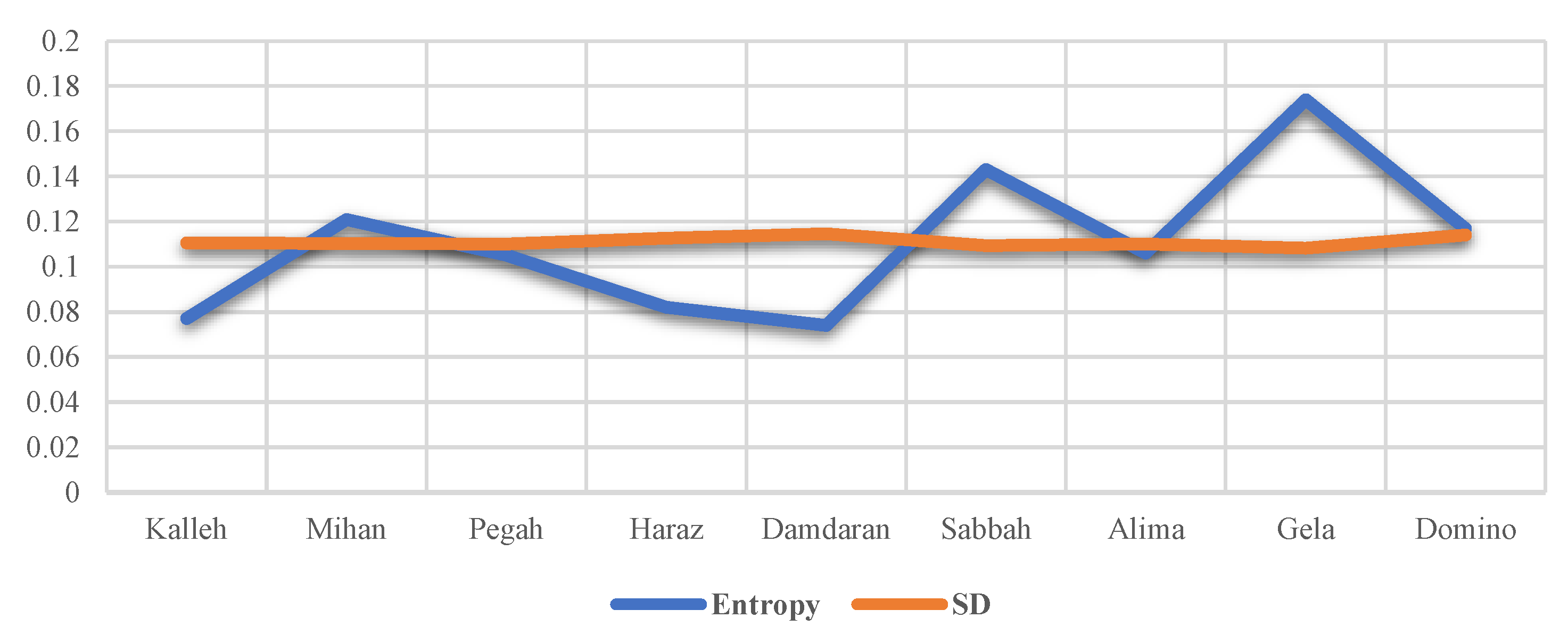
In the case of stability computation of the sustainable supplier selection, the comparison between SD and entropy application in the second case indicates the same result of the supplier evaluation, while the results of the comparison in the first case show the fundamental difference. Furthermore, there are differences in the values of stability derived from two mentioned methods. After the normalization of the ( S S i ) derived from Table 7, Table 12, Table 13 and Table 14, the comparison of stability results obtained from entropy and SD is illustrated in Figure 6 and Figure 7.
The dissimilarities between results of entropy and SD applications could be potentially explained by the different results of stability (see Figure 6). When the numbers of alternatives are limited, both entropy and SD applications show the same performance while in the problem with a large number of alternatives, entropy works more accurately.

Comparison

The computation in ARPASS is based on the quantitative and qualitative values of each criterion. It deals with the qualitative values well, as well as AHP due to their similar pairwise comparison processes. In AHP, by increasing alternatives and criteria, the increasing numbers of calculations may result due to complexity with computation, while in ARPASS, comparison numbers depend on the number of alternatives (see Equation (29)), where ( m ) and ( n ) are the number of alternatives and criteria, respectively.
N u m b e r s   o f   c o m p a r i s o n s   = m 2 n
As Chatterjee et al. [75] and Macharis et al. [76] argued, the main AHP disadvantage is the limitation of the 9-point scale. ARPASS uses the 3-point scale which may seem as an expressible disadvantage, while this limitation is covered by an additional equation as denoted in Equations (13) and (14). In the AHP algorithm, DMs must evaluate the consistency of that matrix (consistency ratio > 0.10), yet ARPASS does not need a rechecking or re-evaluation.
Compared to TOPSIS, VIKOR, and SAW, ARPASS takes more calculation time, while all methods have mathematically moderate complex computations. SAW is known as the simplest MCDM method, and its ranking procedure is based on the highest scores of the weighted summation of the performance rating for each alternative [77].
As mentioned heretofore, ARPASS deals well with both qualitative and quantitative defined values, while the computations in TOPSIS, VIKOR, and SAW algorithms are established on the quantitative values of criteria; the qualitative values can be used in those methods with some numerical scales to translate the linguistic variables into the numbers. According to Chatterjee et al. [75], the complexity of an MCDM method and its transparency are in a direct relationship, directly related. In contrast to the low transparency of AHP due to its high complexity, ARPASS has reasonable transparency since DMs are able to follow each stage of the algorithm to identify any mistakes. Of the mentioned MCDM methods, SAW, TOPSIS, and VIKOR have the best transparency.
To validate the ARPASS result, it is compared with the outputs of SAW, TOPSIS, and VIKOR applied to the cheese supplier selection for the chain store. In Table 17, the given contents demonstrate each method’s results.
As shown in Table 17, Kalleh was selected as the best cheese supplier by all methods, yet the fluctuations in the ranking of other suppliers could be easily detected. The following figure (Figure 8) displays the fluctuations of the first six suppliers in ARPASS, SAW, TOPSIS, and VIKOR, where Kalleh and Haraz are the first two cheese suppliers in each method’s result, and Mihan stands in third place in ARPASS, TOPSIS, and VIKOR.
As portrayed in Figure 8, ARPASS, VIKOR, and TOPSIS selected Kalleh and Haraz as the two first cheese suppliers and SAW selected Kalleh and Pegah as the best. By investigating the results, ARPASS and TOPSIS showed more similarity compared with ARPASS and VIKOR. The prioritization of the first six suppliers in the four mentioned methods is shown in Table 18.
The differentiation of ARPASS and the mentioned method is caused by ( S S j ) calculated by (Equation (12)). In accordance with Table 19, Haraz and Kalleh possess the highest stability among the six selected suppliers.
To reinvestigate the impact of ( S S i ), we ranked suppliers without the impact of ( S S i ). The result is shown in Table 20, where ARPASS* is the ARPASS without the impact of ( S S i ).
The comparison between six selected suppliers is shown in the following table (Table 21).
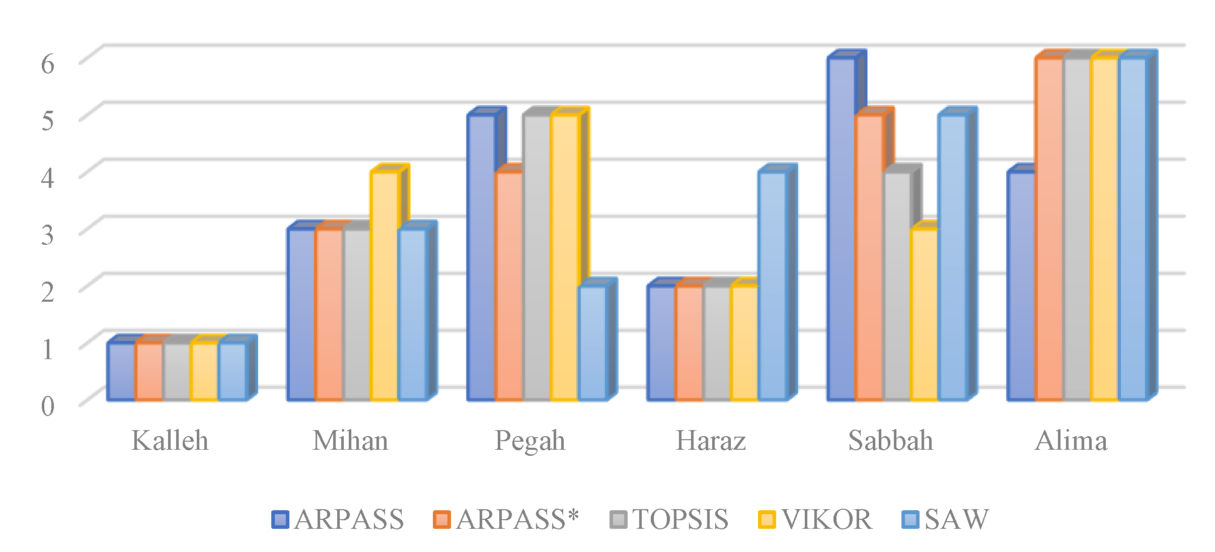
The comparative analysis of the six suppliers’ ranking obtained from ARPASS, TOPSIS, VIKOR, and SAW with ARPASS* is illustrated in (Figure 9).
To compute the stability of the alternatives, ARPASS uses Shannon’s entropy alongside SD (see Section 3.3). As mentioned in Section 3.3, entropy is more useful than SD in the decision-making problem with a large number of alternatives and criteria. We compared the result of ARPASS-E with the results of other mentioned methods where the obtained results are illustrated in Table 22.
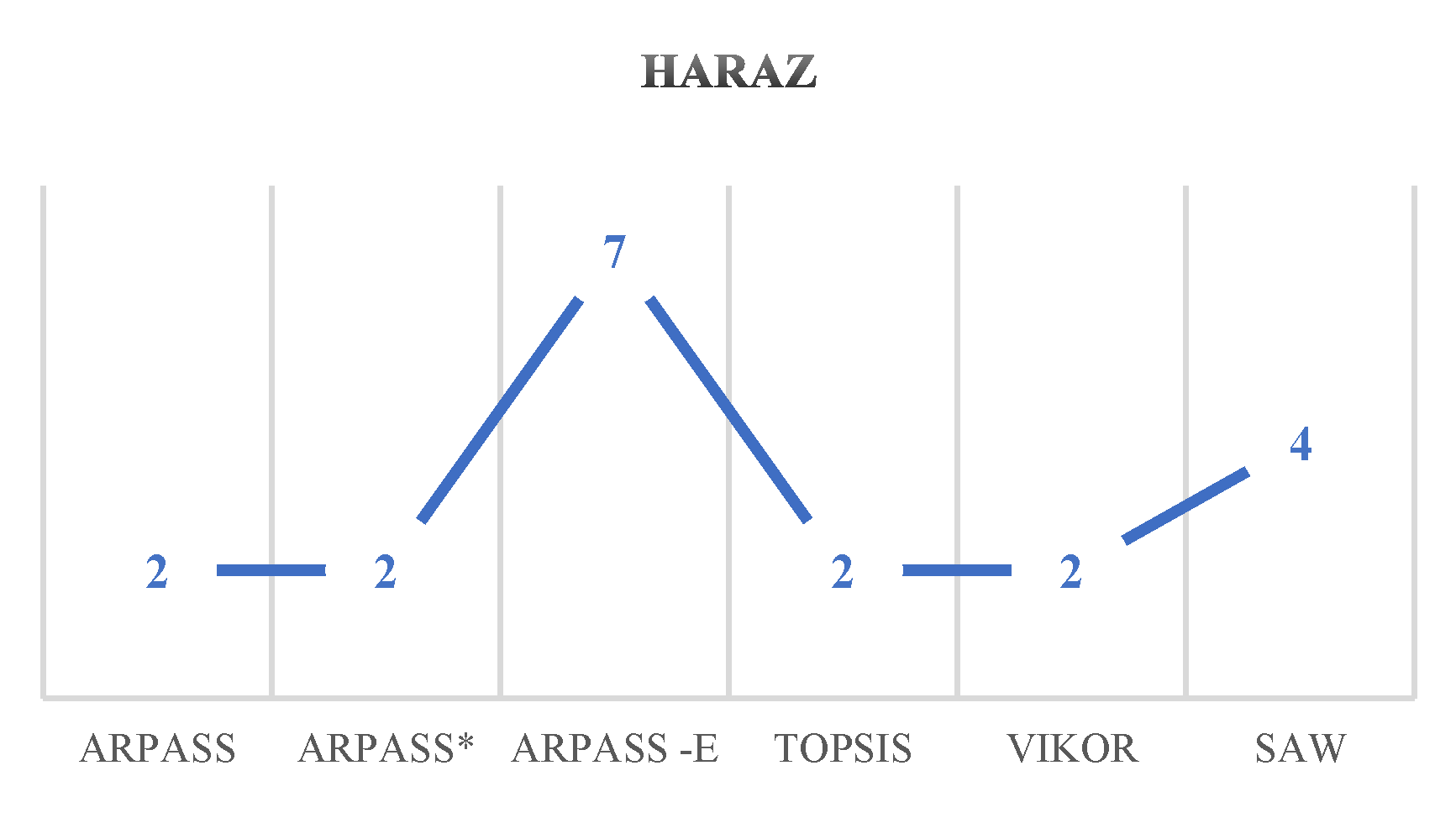
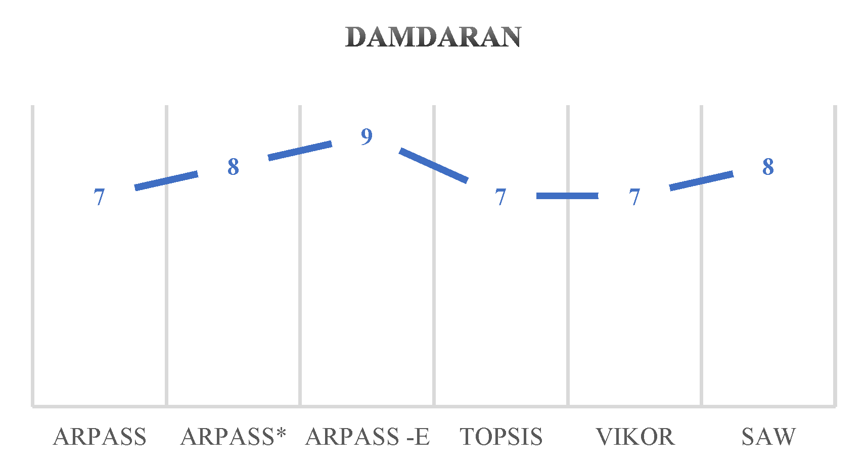
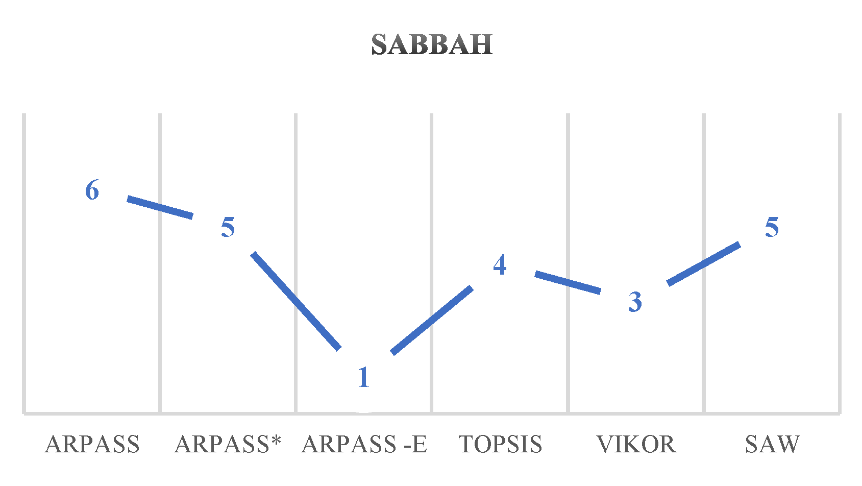
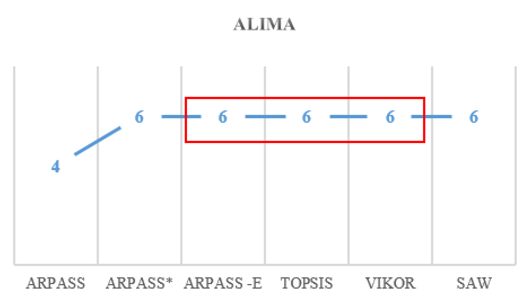
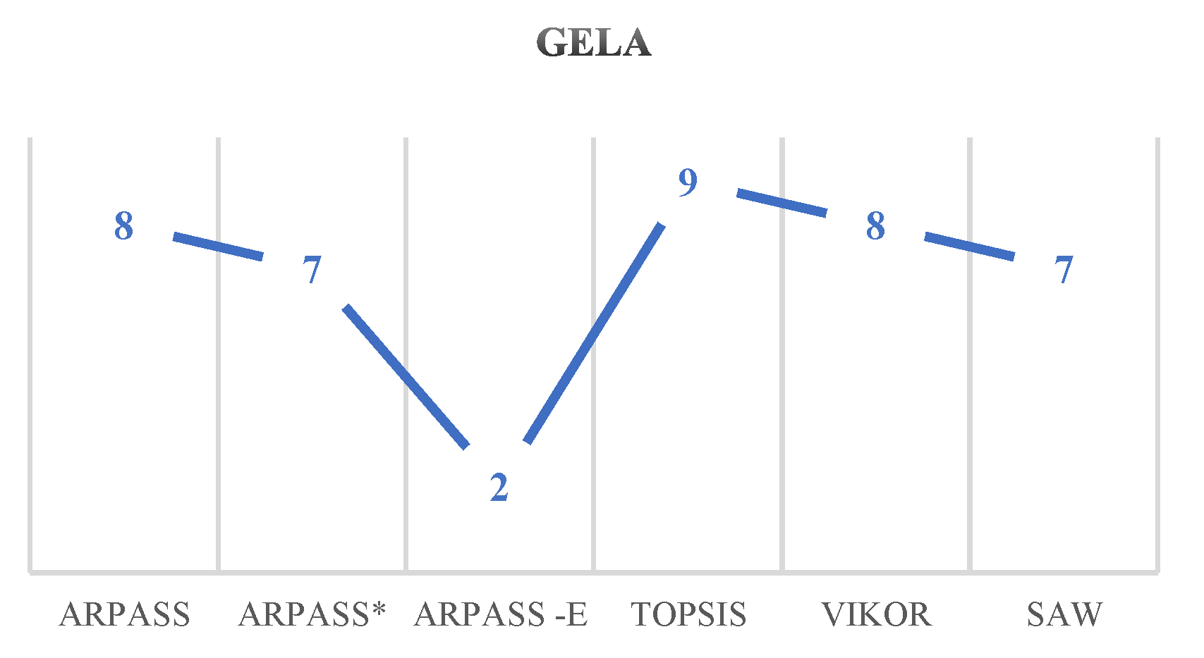
The results of ARPASS-E are completely different than other methods as displayed in Table 22. The impact of stability of each alternative can be clearly found in Figure 10, Figure 11, Figure 12, Figure 13, Figure 14, Figure 15, Figure 16, Figure 17 and Figure 18.
As illustrated in Figure 10, Figure 11, Figure 12, Figure 13, Figure 14, Figure 15, Figure 16, Figure 17 and Figure 18, ARPASS-E has more similarity in ranking with TOPSIS rather than other methods (see the red rectangle in Figure 12, Figure 16 and Figure 18). The ranking result in ARPASS-E has a direct relation with the stability of alternatives. ARPASS-E has also another advantage of selection of the most important criteria that has the most effect on his/her decision.

5. Conclusions and Future Works

Supplier selection is an integral part of supply chain management. Due to the direct impact of the suppliers on the whole firm’s supply chain, selecting the best supplier is a vital decision for the firms. The supplier selection problems deal with evaluating the potential suppliers against several predefined criteria which makes it a typical multi-criteria decision-making (MCDM) problem which is solved by MCDM methods. Various MCDM methods are employed to extract the optimal supplier in the supplier selection problems. In this paper, in order to select the best supplier, two multi-criteria decision-making (MCDM) methods were introduced, called ARPASS and ARPASS*. To evaluate the suppliers, ARPASS deals with the alternatives’ stabilities, obtained from standard deviation or entropy, while ARPASS* does not consider the stability of the suppliers in its algorithm. In MCDM problems, criteria display the alternatives’ common important characteristics. The existing MCDM methods ignore the nature of an alternative as an integrated system, and they merely evaluate the alternatives’ properties against each defined criterion separately. It emanates two major issues related to MCDM problems in general and for the supplier selection in particular. The current trend in solving MCDM problems is centralized on the criteria; hence alternatives are selected based on the most important criterion/criteria, while other characteristics are overshadowed. This issue could be solved by two solutions: 1. The distribution of the weights must be balanced without a wide difference range between the least important criterion and the most important criterion. This requires the execution of a rigorous process for the selection of the problem’s criteria prior to evaluating them and determining their weights. The second solution is the consideration of the independent existence for each alternative as an integrated system where it requires stability to function properly as a potential best alternative. MCDM rating methods are fundamentally designed to evaluate the alternatives; therefore, they could be considered for the second solution. However, as mentioned the existing methods ignore it. As a classic MCDM problem, solving the supplier selection problems is also facing the mentioned issues. Focusing on one criterion or a tiny fraction of the criteria in ranking suppliers eclipses the fact that not only does a supplier need to have a high performance in the important criterion/criteria, but it also requires having a balanced function in all defined characteristics, where we call it the stability of a supplier. As an MCDM method, ARPASS is developed to take the impact of the stability of suppliers on their prioritization into account. To showcase applicability and validate ARPASS and ARPASS*, both methods were applied on two examples of suppliers’ evaluation including a cheese supplier selection problem for a chain store located in Iran and cheese supplier selection for outsourcing production. We compared results of supplier evaluation using ARPASS and ARPASS* with the results obtained from TOPSIS, VIKOR, and SAW as three examples of the popular MCDM methods, considering transparency, complexity, computation time, and information type. The comparative analysis revealed that ARPASS and ARPASS* perform as well as other aforementioned MCDM methods; however, the differences in rankings emerged in both examples which emanated from the impact of the stability coefficient. ARPASS and ARPASS* have salient potential to develop in order to solve decision-making problems; hence, the following suggestions could be considered as interesting future work for researchers. The application of ARPASS and ARPASS* to other real-world problems and comparing the results with other MCDM methods’ results in order to test the possible differences in rankings due to the impact of the stability coefficient could be considered an interesting suggestion for future research. Using the stability philosophy in other MCDM methods as an independent coefficient would be another suggestion for future work. Evaluation of the alternatives by ARPASS under uncertain environments using fuzzy logic and the extensions of the Fuzzy Set could be considered as another suggestion for future research. The use of robust statistics and average absolute deviation in ARPASS algorithms to compute the stability would be interesting for further research. Finally, using GEP in grey numbers’ application and comparing the results with the Moore’s approach [78], Ishibuchi and Tanaka’s model [79], the grey possibility degree [80], Hu and Wang’s approach [81], kernel and degree of greyness of grey numbers model [82], and Xie and Liu’s proposed approach [83] is our last suggestion for future research.

Author Contributions

Conceptualization, S.Z.; methodology, S.Z. and Y.Y.; validation, S.Z. and Y.Y. and D.K.; formal analysis, S.Z.; investigation, S.Z.; resources, S.Z.; writing—original draft preparation, S.Z. and Y.Y.; writing—review and editing, S.Z. and Y.Y. and D.K.; supervision, D.K.; All authors have read and agreed to the published version of the manuscript.

Funding

This research received no external funding.

Informed Consent Statement

Not applicable.

Conflicts of Interest

The authors declare no conflict of interest.

References

  1. Gegovska, T.; Koker, R.; Cakar, T. Green Supplier Selection Using Fuzzy Multiple-Criteria Decision-Making Methods and Artificial Neural Networks. Comput. Intell. Neurosci. 2020, 2020, 8811834. [Google Scholar] [CrossRef] [PubMed]
  2. Quan, J.; Zeng, B.; Liu, D. Green supplier selection for process industries using weighted grey incidence decision model. Complexity 2018, 2018, 4631670. [Google Scholar] [CrossRef]
  3. Ou, Y.; Liu, B. Exploiting the Chain Convenience Store Supplier Selection Based on ANP-MOP Model. Math. Probl. Eng. 2021, 2021, 5582067. [Google Scholar] [CrossRef]
  4. Zakeri, S.; Chatterjee, P.; Cheikhrouhou, N.; Konstantas, D. Ranking based on optimal points and win-loss-draw multi-criteria decision-making with application to supplier evaluation problem. Expert Syst. Appl. 2022, 191, 116258. [Google Scholar] [CrossRef]
  5. Kaur, P.; Dutta, V.; Pradhan, B.L.; Haldar, S.; Chauhan, S. A Pythagorean Fuzzy Approach for Sustainable Supplier Selection Using TODIM. Math. Probl. Eng. 2021, 2021, 4254894. [Google Scholar] [CrossRef]
  6. Zakeri, S.; Keramati, M.A. Systematic combination of fuzzy and grey numbers for supplier selection problem. Grey Syst. Theory Appl. 2015, 5, 313–343. [Google Scholar] [CrossRef]
  7. Zakeri, S.; Ecer, F.; Konstantas, D.; Cheikhrouhou, N. The vital-immaterial-mediocre multi-criteria decision-making method. Kybernetes 2021. ahead-of-print. [Google Scholar] [CrossRef]
  8. Jiang, Y.P.; Liang, H.M.; Sun, M. A method for discrete stochastic MADM problems based on the ideal and nadir solutions. Comput. Ind. Eng. 2015, 87, 114–125. [Google Scholar] [CrossRef]
  9. Zakeri, S. Ranking based on optimal points multi-criteria decision-making method. Grey Syst. Theory Appl. 2019, 9, 45–69. [Google Scholar] [CrossRef]
  10. Keršulienė, V.; Turskis, Z. Integrated fuzzy multiple criteria decision making model for architect selection. Technol. Econ. Dev. Econ. 2011, 17, 645–666. [Google Scholar] [CrossRef]
  11. Toloie-Eshlaghy, A.; Homayonfar, M.; Aghaziarati, M.; Arbabiun, P. A subjective weighting method based on group decision making for ranking and measuring criteria values. Aust. J. Basic Appl. Sci. 2011, 5, 2034–2040. [Google Scholar]
  12. Xu, X. The SIR method: A superiority and inferiority ranking method for multiple criteria decision making. Eur. J. Oper. Res. 2001, 131, 587–602. [Google Scholar] [CrossRef]
  13. Jessop, A. IMP: A decision aid for multiattribute evaluation using imprecise weight estimates. Omega 2014, 49, 18–29. [Google Scholar] [CrossRef] [Green Version]
  14. Rezaei, J. Best-worst multi-criteria decision-making method. Omega 2015, 53, 49–57. [Google Scholar] [CrossRef]
  15. Hwang, C.L.; Yoon, K. Methods for multiple attribute decision making. In Multiple Attribute Decision Making; Springer: Berlin/Heidelberg, Germany, 1981; pp. 58–191. [Google Scholar] [CrossRef]
  16. Saaty, T.L. On polynomials and crossing numbers of complete graphs. J. Comb. Theory Ser. A 1971, 10, 183–184. [Google Scholar] [CrossRef] [Green Version]
  17. Saaty, T.L. What is the analytic hierarchy process? In Mathematical Models for Decision Support; Springer: Berlin/Heidelberg, Germany, 1988; pp. 109–121. [Google Scholar] [CrossRef]
  18. Saaty, T.L. Decision Making with Dependence and Feedback: The Analytic Network Process; RWS Publications: Pittsburgh, PA, USA, 1996; Volume 4922, Available online: http://www.cs.put.poznan.pl/ewgmcda/pdf/SaatyBook.pdf (accessed on 1 October 2021).
  19. MacCrimmon, K.R.; Rand, C. Decision Making among Multiple-Attribute Alternatives: A Survey and Consolidated Approach; Rand Corporation: Santa Monica, CA, USA, 1968. [Google Scholar]
  20. Charnes, A.; Cooper, W.W.; Rhodes, E. Measuring the efficiency of decision making units. Eur. J. Oper. Res. 1978, 2, 429–444. [Google Scholar] [CrossRef]
  21. Opricovic, S. Multicriteria Optimization of Civil Engineering Systems. Ph.D. Thesis, Faculty of Civil Engineering, Belgrade, Serbia, 1998. [Google Scholar]
  22. Opricovic, S.; Tzeng, G.H. Multicriteria planning of post-earthquake sustainable reconstruction. Comput. Aided Civ. Infrastruct. Eng. 2002, 17, 211–220. [Google Scholar] [CrossRef]
  23. Fontela, E.; Gabus, A. The DEMATEL Observer; DEMATEL 1976 Report; Battelle Geneva Research Center: Geneva, Switzerland, 1976. [Google Scholar]
  24. Mareschal, B.; Brans, J.P.; Vincke, P. PROMETHEE: A New Family of Outranking Methods in Multicriteria Analysis. Universite Libre de Bruxelles. 1984. Available online: https://ideas.repec.org/p/ulb/ulbeco/2013-9305.html (accessed on 1 October 2021).
  25. Roy, B. Classement et choix en présence de points de vue multiples. Rev. Française D’informatique Rech. Opérationnelle 1968, 2, 57–75. Available online: http://www.numdam.org/article/RO_1968__2_1_57_0.pdf (accessed on 1 October 2021). [CrossRef]
  26. Roy, B. Problems and methods with multiple objective functions. Math. Program. 1971, 1, 239–266. [Google Scholar] [CrossRef]
  27. Roy, B. ELECTRE III: Un algorithme de classement fondé sur une représentation floue des préférences en présence de critères multiples. Cahiers CERO 1972, 20, 3–24. [Google Scholar]
  28. Roy, B.; Bertier, P. La Méthode ELECTRE II. In Proceedings of the 6ème Conférence Internationale de Recherche Opérationnelle, Dublin, Ireland, 21–25 August 1972. [Google Scholar]
  29. Srisawat, C. Comparison of MCDM methods for intercrop selection in rubber plantations. J. Inf. Commun. Technol. 2020, 15, 165–182. Available online: http://e-journal.uum.edu.my/index.php/jict/article/view/8179 (accessed on 1 October 2021). [CrossRef]
  30. Ghaleb, A.M.; Kaid, H.; Alsamhan, A.; Mian, S.H.; Hidri, L. Assessment and Comparison of Various MCDM Approaches in the Selection of Manufacturing Process. Adv. Mater. Sci. Eng. 2020, 2020, 4039253. [Google Scholar] [CrossRef]
  31. Arabameri, A.; Rezaei, K.; Cerda, A.; Lombardo, L.; Rodrigo-Comino, J. GIS-based groundwater potential mapping in Shahroud plain, Iran. A comparison among statistical (bivariate and multivariate), data mining and MCDM approaches. Sci. Total Environ. 2019, 658, 160–177. [Google Scholar] [CrossRef]
  32. Petrović, G.; Mihajlović, J.; Ćojbašić, Ž.; Madić, M.; Marinković, D. Comparison of three fuzzy MCDM methods for solving the supplier selection problem. Facta Univ. Ser. Mech. Eng. 2019, 17, 455–469. [Google Scholar] [CrossRef]
  33. Munier, N.; Hontoria, E.; Jiménez-Sáez, F. Analysis of Lack of Agreement Between MCDM Methods Related to the Solution of a Problem: Proposing a Methodology for Comparing Methods to a Reference. In Strategic Approach in Multi-Criteria Decision Making; Springer: Berlin/Heidelberg, Germany, 2019; pp. 203–219. [Google Scholar] [CrossRef]
  34. Tarmudi, Z.; Rahman, N.A. Diverse Ranking Approach in MCDM Based on Trapezoidal Intuitionistic Fuzzy Numbers. In Proceedings of the International Conference on Soft Computing and Pattern Recognition, Porto, Portugal, 13–15 December 2018; Springer: Berlin/Heidelberg, Germany, 2018; pp. 11–21. [Google Scholar] [CrossRef]
  35. Zamani-Sabzi, H.; King, J.P.; Gard, C.C.; Abudu, S. Statistical and analytical comparison of multi-criteria decision-making techniques under fuzzy environment. Oper. Res. Perspect. 2016, 3, 92–117. [Google Scholar] [CrossRef] [Green Version]
  36. Kralik, L.; Senkerik, R.; Jasek, R. Comparison of MCDM methods with users’ evaluation. In Proceedings of the 11th Iberian Conference on Information Systems and Technologies, Gran Canaria, Spain, 15–18 June 2016; pp. 1–5. [Google Scholar] [CrossRef]
  37. Zakeri, S.; Yang, Y.; Hashemi, M. Grey strategies interaction model. J. Strategy Manag. 2019, 12, 30–60. [Google Scholar] [CrossRef]
  38. Rashidi, K.; Cullinane, K. A comparison of fuzzy DEA and fuzzy TOPSIS in sustainable supplier selection: Implications for sourcing strategy. Expert Syst. Appl. 2019, 121, 266–281. [Google Scholar] [CrossRef]
  39. Yu, C.; Shao, Y.; Wang, K.; Zhang, L. A group decision making sustainable supplier selection approach using extended TOPSIS under interval-valued Pythagorean fuzzy environment. Expert Syst. Appl. 2019, 121, 1–17. [Google Scholar] [CrossRef]
  40. Karami, S.; Ghasemy Yaghin, R.; Mousazadegan, F. Supplier selection and evaluation in the garment supply chain: An integrated DEA–PCA–VIKOR approach. J. Text. Inst. 2020, 112, 578–595. [Google Scholar] [CrossRef]
  41. Zhang, J.; Yang, D.; Li, Q.; Lev, B.; Ma, Y. Research on sustainable supplier selection based on the rough DEMATEL and FVIKOR methods. Sustainability 2020, 13, 88. [Google Scholar] [CrossRef]
  42. Choo, E.U.; Wedley, W.C. A common framework for deriving preference values from pairwise comparison matrices. Comput. Oper. Res. 2004, 31, 893–908. [Google Scholar] [CrossRef]
  43. Chen, T. A diversified AHP-tree approach for multiple-criteria supplier selection. Comput. Manag. Sci. 2021, 18, 431–453. [Google Scholar] [CrossRef]
  44. Fagundes, M.V.; Hellingrath, B.; Freires, F.G. Supplier selection risk: A new computer-based decision-making system with fuzzy extended AHP. Logistics 2021, 5, 13. [Google Scholar] [CrossRef]
  45. Unal, Y.; Temur, G.T. Using Spherical Fuzzy AHP Based Approach for Prioritization of Criteria Affecting Sustainable Supplier Selection. In Proceedings of the International Conference on Intelligent and Fuzzy Systems, Istanbul, Turkey, 21–23 July 2020; pp. 160–168. [Google Scholar] [CrossRef]
  46. Wang, Y.C.; Chen, T. A Bi-objective AHP-MINLP-GA approach for Flexible Alternative Supplier Selection amid the COVID-19 pandemic. Soft Comput. Lett. 2021, 3, 100016. [Google Scholar] [CrossRef]
  47. Tong, L.Z.; Wang, J.; Pu, Z. Sustainable supplier selection for SMEs based on an extended PROMETHEE Ⅱ approach. J. Clean. Prod. 2022, 330, 129830. [Google Scholar] [CrossRef]
  48. Tong, L.; Pu, Z.; Chen, K.; Yi, J. Sustainable maintenance supplier performance evaluation based on an extend fuzzy PROMETHEE II approach in petrochemical industry. J. Clean. Prod. 2020, 273, 122771. [Google Scholar] [CrossRef]
  49. Stević, Ž.; Pamučar, D.; Puška, A.; Chatterjee, P. Sustainable supplier selection in healthcare industries using a new MCDM method: Measurement of alternatives and ranking according to Compromise solution (MARCOS). Comput. Ind. Eng. 2020, 140, 106231. [Google Scholar] [CrossRef]
  50. Jain, N.; Singh, A.R.; Upadhyay, R.K. Sustainable supplier selection under attractive criteria through FIS and integrated fuzzy MCDM techniques. Int. J. Sustain. Eng. 2020, 13, 441–462. [Google Scholar] [CrossRef]
  51. Çalık, A. A novel Pythagorean fuzzy AHP and fuzzy TOPSIS methodology for green supplier selection in the Industry 4.0 era. Soft Comput. 2021, 25, 2253–2265. [Google Scholar] [CrossRef]
  52. Tavassoli, M.; Saen, R.F.; Zanjirani, D.M. Assessing sustainability of suppliers: A novel stochastic-fuzzy DEA model. Sustain. Prod. Consum. 2020, 21, 78–91. [Google Scholar] [CrossRef]
  53. Nemati, M.; Saen, R.F.; Matin, R.K. A data envelopment analysis approach by partial impacts between inputs and desirable-undesirable outputs for sustainable supplier selection problem. Ind. Manag. Data Syst. 2020, 121, 809–838. [Google Scholar] [CrossRef]
  54. Davoudabadi, R.; Mousavi, S.M.; Sharifi, E. An integrated weighting and ranking model based on entropy, DEA and PCA considering two aggregation approaches for resilient supplier selection problem. J. Comput. Sci. 2020, 40, 101074. [Google Scholar] [CrossRef]
  55. Ratna, S.; Bhat, M.; Singh, N.P.; Saxena, M.; Misra, S.; Vishwakarma, P.N.; Kumar, B. Sustainable Supplier Selection in Automobile Sector Using GRA–TOP Model. In Advances in Industrial and Production Engineering; Springer: Berlin/Heidelberg, Germany, 2021; pp. 393–400. [Google Scholar] [CrossRef]
  56. Bali, O.; Kose, E.; Gumus, S. Green supplier selection based on IFS and GRA. Grey Syst. Theory Appl. 2013, 3, 158–176. [Google Scholar] [CrossRef]
  57. Giri, B.C.; Molla, M.U.; Biswas, P. Pythagorean fuzzy DEMATEL method for supplier selection in sustainable supply chain management. Expert Syst. Appl. 2022, 193, 116396. [Google Scholar] [CrossRef]
  58. Chen, Z.; Ming, X.; Zhou, T.; Chang, Y. Sustainable supplier selection for smart supply chain considering internal and external uncertainty: An integrated rough-fuzzy approach. Appl. Soft Comput. 2020, 87, 106004. [Google Scholar] [CrossRef]
  59. Chen, C.H. A Hybrid Multi-Criteria Decision-Making Approach Based on ANP-Entropy TOPSIS for Building Materials Supplier Selection. Entropy 2021, 23, 1597. [Google Scholar] [CrossRef]
  60. Abdel-Baset, M.; Chang, V.; Gamal, A.; Smarandache, F. An integrated neutrosophic ANP and VIKOR method for achieving sustainable supplier selection: A case study in importing field. Comput. Ind. 2019, 106, 94–110. [Google Scholar] [CrossRef]
  61. Masoomi, B.; Sahebi, I.G.; Fathi, M.; Yıldırım, F.; Ghorbani, S. Strategic supplier selection for renewable energy supply chain under green capabilities (fuzzy BWM-WASPAS-COPRAS approach). Energy Strategy Rev. 2022, 40, 100815. [Google Scholar] [CrossRef]
  62. Rani, P.; Mishra, A.R.; Krishankumar, R.; Mardani, A.; Cavallaro, F.; Soundarapandian Ravichandran, K.; Balasubramanian, K. Hesitant Fuzzy SWARA-Complex Proportional Assessment Approach for Sustainable Supplier Selection (HF-SWARA-COPRAS). Symmetry 2020, 12, 1152. [Google Scholar] [CrossRef]
  63. Qu, G.; Zhang, Z.; Qu, W.; Xu, Z. Green supplier selection based on green practices evaluated using fuzzy approaches of TOPSIS and ELECTRE with a case study in a Chinese Internet company. Int. J. Environ. Res. Public Health 2020, 17, 3268. [Google Scholar] [CrossRef]
  64. Govindan, K.; Kadziński, M.; Ehling, R.; Miebs, G. Selection of a sustainable third-party reverse logistics provider based on the robustness analysis of an outranking graph kernel conducted with ELECTRE I and SMAA. Omega 2019, 85, 1–15. [Google Scholar] [CrossRef]
  65. Vojinović, N.; Sremac, S.; Zlatanović, D. A Novel Integrated Fuzzy-Rough MCDM Model for Evaluation of Companies for Transport of Dangerous Goods. Complexity 2021, 2021, 5141611. [Google Scholar] [CrossRef]
  66. Tian, X.; Niu, M.; Ma, J.; Xu, Z. A novel TODIM with probabilistic hesitant fuzzy information and its application in green supplier selection. Complexity 2020, 2020, 2540798. [Google Scholar] [CrossRef]
  67. Qin, Z. Random fuzzy mean-absolute deviation models for portfolio optimization problem with hybrid uncertainty. Appl. Soft Comput. 2017, 56, 597–603. [Google Scholar] [CrossRef]
  68. Shrestha, P.; Park, Y.; Kwon, H.; Kim, C.G. Error outlier with weighted Median Absolute Deviation threshold algorithm and FBG sensor based impact localization on composite wing structure. Compos. Struct. 2017, 180, 412–419. [Google Scholar] [CrossRef]
  69. Mukhopadhyay, N.; Hu, J. Confidence intervals and point estimators for a normal mean under purely sequential strategies involving Gini’s mean difference and mean absolute deviation. Seq. Anal. 2017, 36, 210–239. [Google Scholar] [CrossRef]
  70. Ma, W.; Zheng, D.; Zhang, Z.; Chen, B. Bias-compensated normalized least mean absolute deviation algorithm with noisy input. In Proceedings of the 20th International Conference on Information Fusion, Xi’an, China, 10–13 July 2017; pp. 1–5. [Google Scholar] [CrossRef]
  71. Denneberg, D. Premium Calculation: Why Standard Deviation Should be Replaced by Absolute Deviation1. ASTIN Bull. J. IAA 1990, 20, 181–190. [Google Scholar] [CrossRef] [Green Version]
  72. Deng, J.L. Introduction to grey system theory. J. Grey Syst. 1989, 1, 1–24. [Google Scholar]
  73. Deng, J.L. Fundamental Methods of Grey Systems; Huazhoug University of Science and Technology: Wuhan, China, 1985. [Google Scholar]
  74. Zakeri, S.; Konstantas, D.; Cheikhrouhou, N. The Grey Ten-Element Analysis Method: A Novel Strategic Analysis Tool. Mathematics 2022, 10, 846. [Google Scholar] [CrossRef]
  75. Chatterjee, P.; Athawale, V.M.; Chakraborty, S. Materials selection using complex proportional assessment and evaluation of mixed data methods. Mater. Des. 2011, 32, 851–860. [Google Scholar] [CrossRef]
  76. Macharis, C.; Springael, J.; De Brucker, K.; Verbeke, A. PROMETHEE and AHP: The design of operational synergies in multicriteria analysis: Strengthening PROMETHEE with ideas of AHP. Eur. J. Oper. Res. 2004, 153, 307–317. [Google Scholar] [CrossRef]
  77. Xu, F.; Liu, J.; Lin, S.; Yuan, J. A VIKOR-based approach for assessing the service performance of electric vehicle sharing programs: A case study in Beijing. J. Clean. Prod. 2017, 148, 254–267. [Google Scholar] [CrossRef]
  78. Moore, R.E. Method and Application of Interval Analysis; Society for Industrial and Applied Math: Philadelphia, PA, USA, 1979; pp. 74–79. [Google Scholar]
  79. Ishibuchi, H.; Tanaka, H. Multiobjective programming in optimization of the interval objective function. Eur. J. Oper. Res. 1990, 48, 219–225. [Google Scholar] [CrossRef]
  80. Li, G.D.; Yamaguchi, D.; Nagai, M. A grey-based decision-making approach to the supplier selection problem. Math. Comput. Model. 2007, 46, 573–581. [Google Scholar] [CrossRef]
  81. Hu, B.Q.; Wang, S. A novel approach in uncertain programming part i: New arithmetic and order relation for interval numbers. J. Ind. Manag. Optim. 2006, 2, 351. [Google Scholar] [CrossRef]
  82. Xie, N.M.; Liu, S.F. Novel methods on comparing grey numbers. Appl. Math. Model. 2010, 34, 415–423. [Google Scholar] [CrossRef]
  83. Xie, N.M.; Liu, S.F. On comparing grey numbers with their probability distribution. Syst. Eng. Theory Pract. 2009, 29, 169–175. [Google Scholar]
Figure 1. The bigfoot monster truck.
Processes 10 00917 g001
Figure 2. A typical truck.
Processes 10 00917 g002
Figure 3. The variation in each alternative in the normalized decision matrix, where A 1 , A 2 , and A 3 are the alternatives.
Processes 10 00917 g003
Figure 4. The variation in each alternative in the weighted normalized decision matrix, where A 1 , A 2 , and A 3 are the alternatives.
Processes 10 00917 g004
Figure 5. The transformed decision matrix for the computation of each alternative’s stability with entropy.
Processes 10 00917 g005
Figure 6. The comparison of SD and entropy in the case of stability computation: first suppliers’ evaluation example.
Processes 10 00917 g006
Figure 7. The comparison of SD and entropy in the case of stability computation: the second suppliers’ evaluation example.
Processes 10 00917 g007
Figure 8. The comparative analysis for the first cheese suppliers of ARASS, TOPSIS, VIKOR, and SAW.
Processes 10 00917 g008
Figure 9. Comparative analysis of ranking results of the first six suppliers.
Processes 10 00917 g009
Figure 10. Rank fluctuation of Kalleh in the investigated MCDM methods.
Processes 10 00917 g010
Figure 11. Rank fluctuation of Mihan in the six investigated methods.
Processes 10 00917 g011
Figure 12. Rank fluctuation of Pegah in the investigated MCDM methods.
Processes 10 00917 g012
Figure 13. Rank fluctuation of Haraz in the investigated MCDM methods.
Processes 10 00917 g013
Figure 14. Rank fluctuation of Damdaran in the investigated MCDM methods.
Processes 10 00917 g014
Figure 15. Rank fluctuation of Sabbah in the investigated MCDM methods.
Processes 10 00917 g015
Figure 16. Rank fluctuation of Alima in the investigated MCDM methods.
Processes 10 00917 g016
Figure 17. Rank fluctuation of Gela in the investigated MCDM methods.
Processes 10 00917 g017
Figure 18. Rank fluctuation of Domino in the investigated MCDM methods.
Processes 10 00917 g018
Table 1. A decision matrix with random variables.
C 1 C 2 C 3 C 4 C 5
A 1 53500265239
A 2 72300216385
A 3 91950219927
Table 2. An overview of the alternative’s comparison in the ARPASS method. The values in yellow cells are the repetition of the equations.
C j A 1 A 2 A n 1 A n
A 1 3
A 2 C V 12 3
3
A m 1 C V 1 m 1 C V 2 m 1 3
A m C V 1 m C V 2 m C V n 1 m 3
Table 5. Linguistic variables for rating and weighting of criteria.
Scales for Rating the Alternative against CriteriaScales for Weighting the Criteria
Linguistic VariablesNumerical ValueLinguistic VariablesNumerical Value
Very poor (VP)1Very low (VL)0.1
Poor (P)2Low (L)0.2
Medium poor (MP)3Medium low (ML)0.3
Fair (F)5Medium (M)0.5
Medium good (MG)7Medium high (MH)0.7
Good (G)9High (H)0.9
Very good (VG)10Very high (VH)1
Table 6. Supplier evaluation decision matrix.
+++++++++
Appropriateness of the Product Price to the Market PriceNumbers of Promotion TimesAbility to Adapt to
Increase,
Decrease, and Change in
Order Timing
Make-to-Order ProductionDelivery ReliabilityVarietyBrand EquityDefect RATEReliability of QualityAfter Sales Services
Kalleh1012910109100.04879
Mihan914777390.02177
Pegah10129107790.09055
Haraz912979770.04377
Damdaran79577570.05477
Sabbah918799750.04175
Alima56101010950.06395
Gela1012957320.047105
Domino710555270.02957
Table 7. Ranking of the cheese suppliers.
S S j C 1 C 2 C 3 C 4 C 5 C 6 C 7 C 8 C 9 C 10 C S j A V j Rank
2.564Kalleh1012910109100.8907935.403549.831
2.557Mihan914777390.9527728.932502.3713
2.552Pegah10129107790.7945526.882448.7474
2.611Haraz912979770.9017728.792647.8082
2.656Damdaran79577570.8767721.431826.838
2.536Sabbah918799750.9067527.322413.7016
2.552Alima56101010950.8569527.552416.3045
2.509Gela1012957320.89210524.611871.5277
2.643Domino710555270.9335718.201425.4189
Table 8. The grey linguistic variables.
ScaleVery Poor (VP)Poor (P)Medium Poor (MP)Fair (F)Medium Good (MG)Good (G)Very Good (VG)
Grey[0, 1][1, 3][3, 4][4, 5][5, 7][7, 9][9, 10]
Table 9. The GEPs of the grey linguistic variables.
ScaleVery Poor (VP)Poor (P)Medium Poor (MP)Fair (F)Medium Good (MG)Good (G)Very Good (VG)
Grey[0, 1][1, 3][3, 4][4, 5][5, 7][7, 9][9, 10]
Z 0.52.29213.74154.70116.13738.0589.5005
Table 12. The GEP of each nutritional content.
Nutritional ContentFatpHSaltDM
Standard content2450.933
Acceptable interval 22 ,   26 4.8 ,   5.1 0.6 ,   1.1 32 ,   38
α 0.50.20.20.7
β 0.90.50.30.9
GEP23.4144.9810.78533.8
Minimum acceptable content23.4144.9810.78533.8
Table 13. Suppliers’ evaluations with the four conditions of fat, pH, salt, and DM.
FatpHSaltDM
Conditions23.4144.9810.78533.8
α 0.20.20.20.05
β 0.90.50.30.95
S 2 23.94.980.733.71
S 4 22.864.660.5633.94
S 7 23.814.620.7433.99
S 9 23.624.660.5233.94
S 12 23.014.80.5833.52
S 13 23.94.520.6433
S 17 23.954.620.6334.13
S 19 23.814.40.6333.76
Table 14. Ranking of the cheese suppliers.
S S j SuppliersFatpHSaltDM A V i × 10 6 Rank
9.05 S 7 23.814.620.7433.991255.8412
9.08 S 9 23.624.660.5233.94178.4353
9.03 S 17 23.954.620.6334.1320,129.321
Table 15. The normalized transformed benefit matrix, entropy ( E j ), ( S S i ), and the final ranking of the cheese suppliers of the first example.
KallehMihanPegahHarazDamdaranSabbahAlimaGelaDomino
C 1 0.1080.1140.1170.1110.1070.1090.0820.1260.115
C 2 0.1190.1390.1270.1270.1220.1480.0920.1360.136
C 3 0.1020.0990.1110.1110.0880.0950.1210.1200.096
C 4 0.1080.0990.1170.0960.1070.1090.1210.0870.096
C 5 0.1080.0990.0960.1110.1070.1090.1210.1050.096
C 6 0.1020.0580.0960.0960.0880.0950.1150.0620.053
C 7 0.1080.1140.1110.0960.1070.0770.0820.0470.115
C 8 0.0200.0250.0210.0230.0260.0230.0230.0260.030
C 9 0.0880.0990.0790.0960.1070.0950.1150.1260.096
C 10 0.1020.0990.0790.0960.1070.0770.0820.0870.115
S S i C 1 C 2 C 3 C 4 C 5 C 6 C 7 C 8 C 9 C 10 C S i A V i Rank
0.077Kalleh1012910109100.8907935.4051.4713
0.121Mihan914777390.9527728.9350.8314
0.105Pegah10129107790.7945526.8850.4385
0.082Haraz912979770.9017728.7946.3927
0.074Damdaran79577570.8767721.4340.2729
0.143Sabbah918799750.9067527.3255.9111
0.106Alima56101010950.8569527.5548.8466
0.174Gela1012957320.89210524.6152.9222
0.117Domino710555270.9335718.2041.6068
Table 16. The normalized transformed benefit matrix, entropy ( E j ), ( S S i ), and the final ranking of the cheese suppliers of the second example.
S 7 S 9 S 17
Fat0.37700.37650.3782
pH0.07310.07430.0730
Salt0.01170.00830.0099
DM0.53820.54100.5389
S 7 S 9 S 17
E j 0.6810.6730.676
S S i 0.3290.3370.334
S S i SuppliersFatpHSaltDM A V i Rank
0.329 S 7 23.814.620.7433.998.5962
0.337 S 9 23.624.660.5233.948.4513
0.334 S 17 23.954.620.6334.139.8601
Table 17. The ranking results in ARPASS, TOPSIS, SAW, and VIKOR methods.
ARPASSTOPSISVIKORSAW
Kalleh1111
Mihan3343
Pegah5552
Haraz2224
Damdaran7778
Sabbah6435
Alima4666
Gela8987
Domino9899
Table 18. The ranking result of the first six suppliers.
ARPASSTOPSISVIKORSAW
Kalleh1111
Mihan3343
Pegah5552
Haraz2224
Sabbah6435
Alima4666
Table 19. The stability scores of the first five selected suppliers derived from Table 6.
HarazKallehMihanPegahAlimaSabbah
S S j 2.6112.5642.5572.5522.5522.536
Table 20. The ranking results in ARPASS, TOPSIS, SAW, VIKOR, and ARPASS* methods.
ARPASSARPASS*TOPSISVIKORSAW
Kalleh11111
Mihan33343
Pegah54552
Haraz22224
Damdaran78778
Sabbah65435
Alima46666
Gela87987
Domino99899
Table 21. The ranking results of the first six suppliers.
ARPASSARPASS*TOPSISVIKORSAW
Kalleh11111
Mihan33343
Pegah54552
Haraz22224
Sabbah65435
Alima46666
Table 22. The ranking results in ARPASS, TOPSIS, SAW, VIKOR, and ARPASS* methods where ARPASS-E.
ARPASSARPASS*ARPASS -ETOPSISVIKORSAW
Kalleh113111
Mihan334343
Pegah545552
Haraz227224
Damdaran789778
Sabbah651435
Alima466666
Gela872987
Domino998899
Publisher’s Note: MDPI stays neutral with regard to jurisdictional claims in published maps and institutional affiliations.