
A Supplier Selection Model Using Alternative Ranking Process by Alternatives’ Stability Scores and the Grey Equilibrium Product


Abstract
:1. Introduction
2. Materials and Methods
2.1. A Ranking Process by Alternatives’ Stability Scores (ARPASS) Method
| Algorithm 1 |
| for if (), (), and (), then (), (), and (). end if end for Thus for if then the corresponding value is ; else if then the corresponding value is ; else if then the corresponding value is 1. end if end if end for |

| CN | W | D | L | ||
|---|---|---|---|---|---|
2.2. Steps of ARPASS
2.2.1. The First Stage
2.2.2. The Second Stage
2.3. ARPASS-E
2.4. ARPASS*
2.5. Grey Numbers and the Grey Equilibrium Product (GEP)
3. Results
3.1. Example 1: The Evaluation of Chain Store’s Cheese Suppliers
3.1.1. Data Collection
3.1.2. Application and Results
3.2. Example 2: The Cream Cheese Supplier Selection for Outsourcing Production
Application and Results
| G | F | F | VG | VG | F | G | G | F | VG | G | VG | G | VG | VG | VG | F | F | G | G | G | F | G | G | F | G | F | MP | F | G | |
| F | G | G | VG | F | VG | G | F | F | VG | G | F | G | VG | VG | VG | VG | VG | VG | VG | VG | G | G | G | G | G | G | F | G | F | |
| VG | G | G | F | F | F | G | VG | F | F | G | F | G | G | VG | F | F | G | G | VG | VG | VG | G | G | G | G | G | F | F | G | |
| VG | VG | F | VG | VG | G | G | G | G | VG | F | G | G | VG | VG | VG | G | VG | G | VG | VG | G | G | G | G | VG | G | G | G | G | |
| G | VG | F | VG | VG | G | G | G | G | G | F | G | G | G | G | F | G | G | F | G | VG | G | G | G | G | F | G | G | G | G | |
| F | G | G | VG | F | G | G | F | G | F | G | G | F | MP | F | F | G | F | G | VG | VG | G | G | G | G | F | G | G | F | G | |
| VG | G | G | VG | VG | F | G | G | G | VG | G | G | G | VG | VG | VG | G | VG | VG | VG | VG | G | G | G | G | G | G | F | F | G | |
| VG | G | G | VG | G | F | G | G | G | VG | G | F | G | VG | VG | VG | F | G | G | F | G | G | G | G | G | G | G | G | G | G | |
| G | G | G | VG | G | VG | G | G | F | G | F | VG | F | VG | VG | VG | VG | VG | G | VG | VG | G | F | G | G | F | VG | G | F | F | |
| VG | F | F | VG | VG | G | G | VG | G | G | F | G | G | VG | VG | VG | F | F | F | VG | VG | G | G | G | G | G | G | G | G | G | |
| F | G | G | G | F | VG | G | F | G | F | G | F | MP | F | F | G | G | G | G | VG | VG | F | G | G | G | G | G | G | G | G | |
| VG | G | VG | F | VG | F | G | VG | G | G | G | G | G | VG | VG | VG | VG | VG | VG | VG | VG | G | G | G | G | G | F | VG | G | G | |
| F | VG | G | VG | VG | VG | G | F | G | VG | G | VG | G | VG | VG | VG | VG | VG | VG | VG | VG | F | G | G | F | G | VG | MP | F | F | |
| G | G | G | VG | G | F | G | G | G | VG | F | G | F | G | G | F | G | VG | F | G | VG | VG | G | G | G | G | G | F | G | G | |
| F | G | G | VG | G | G | G | F | F | VG | G | G | G | VG | VG | VG | F | VG | VG | G | G | F | G | G | G | G | F | F | G | G | |
| G | G | G | F | G | F | G | G | G | F | G | VG | F | F | G | F | G | G | G | G | F | G | G | G | G | G | F | MP | F | G | |
| VG | VG | G | VG | G | F | G | VG | G | G | G | G | G | VG | VG | VG | G | VG | VG | VG | VG | VG | G | G | G | G | G | VG | G | G | |
| VG | F | VG | VG | F | VG | G | G | G | G | G | G | G | VG | VG | VG | VG | VG | G | G | G | F | G | G | F | G | G | G | F | G | |
| VG | VG | G | VG | F | G | G | VG | F | G | F | G | G | VG | VG | VG | G | VG | VG | VG | VG | F | G | G | G | VG | G | G | F | F | |
| G | VG | VG | VG | F | G | G | F | G | F | G | G | G | F | F | F | G | G | G | G | G | VG | G | G | G | G | F | G | F | G |
| 4.7 | 8.06 | 8.058 | 9.501 | 4.701 | 9.501 | 8.06 | 4.701 | 4.7 | 9.5 | 8.06 | 4.7 | 8.06 | 9.5 | 9.5 | 9.5 | 9.5 | 9.5 | 9.5 | 9.5 | 9.5 | 8.06 | 8.06 | 8.06 | 8.06 | 8.06 | 8.06 | 4.7 | 8.06 | 4.7 | 234.109 | |
| 9.5 | 9.5 | 4.701 | 9.501 | 9.501 | 8.058 | 8.06 | 8.058 | 8.06 | 9.5 | 4.7 | 8.06 | 8.06 | 9.5 | 9.5 | 9.5 | 8.06 | 9.5 | 8.06 | 9.5 | 9.5 | 8.06 | 8.06 | 8.06 | 8.06 | 9.5 | 8.06 | 8.06 | 8.06 | 8.06 | 252.336 | |
| 9.5 | 8.06 | 8.058 | 9.501 | 9.501 | 4.701 | 8.06 | 8.058 | 8.06 | 9.5 | 8.06 | 8.06 | 8.06 | 9.5 | 9.5 | 9.5 | 8.06 | 9.5 | 9.5 | 9.5 | 9.5 | 8.06 | 8.06 | 8.06 | 8.06 | 8.06 | 8.06 | 4.7 | 4.7 | 8.06 | 247.537 | |
| 8.06 | 8.06 | 8.058 | 9.501 | 8.058 | 9.501 | 8.06 | 8.058 | 4.7 | 8.06 | 4.7 | 9.5 | 4.7 | 9.5 | 9.5 | 9.5 | 9.5 | 9.5 | 8.06 | 9.5 | 9.5 | 8.06 | 4.7 | 8.06 | 8.06 | 4.7 | 9.5 | 8.06 | 4.7 | 4.7 | 234.109 | |
| 9.5 | 8.06 | 9.501 | 4.701 | 9.501 | 4.701 | 8.06 | 9.501 | 8.06 | 8.06 | 8.06 | 8.06 | 8.06 | 9.5 | 9.5 | 9.5 | 9.5 | 9.5 | 9.5 | 9.5 | 9.5 | 8.06 | 8.06 | 8.06 | 8.06 | 8.06 | 4.7 | 9.5 | 8.06 | 8.06 | 250.422 | |
| 4.7 | 9.5 | 8.058 | 9.501 | 9.501 | 9.501 | 8.06 | 4.701 | 8.06 | 9.5 | 8.06 | 9.5 | 8.06 | 9.5 | 9.5 | 9.5 | 9.5 | 9.5 | 9.5 | 9.5 | 9.5 | 4.7 | 8.06 | 8.06 | 4.7 | 8.06 | 9.5 | 3.74 | 4.7 | 4.7 | 238.92 | |
| 9.5 | 9.5 | 8.058 | 9.501 | 8.058 | 4.701 | 8.06 | 9.501 | 8.06 | 8.06 | 8.06 | 8.06 | 8.06 | 9.5 | 9.5 | 9.5 | 8.06 | 9.5 | 9.5 | 9.5 | 9.5 | 9.5 | 8.06 | 8.06 | 8.06 | 8.06 | 8.06 | 9.5 | 8.06 | 8.06 | 257.136 | |
| 9.5 | 9.5 | 8.058 | 9.501 | 4.701 | 8.058 | 8.06 | 9.501 | 4.7 | 8.06 | 4.7 | 8.06 | 8.06 | 9.5 | 9.5 | 9.5 | 8.06 | 9.5 | 9.5 | 9.5 | 9.5 | 4.7 | 8.06 | 8.06 | 8.06 | 9.5 | 8.06 | 8.06 | 4.7 | 4.7 | 238.909 |
3.3. Application of Shannon’s Entropy in ARPASS (ARPASS-E)
4. Discussion
Comparison
5. Conclusions and Future Works
Author Contributions
Funding
Informed Consent Statement
Conflicts of Interest
References
- Gegovska, T.; Koker, R.; Cakar, T. Green Supplier Selection Using Fuzzy Multiple-Criteria Decision-Making Methods and Artificial Neural Networks. Comput. Intell. Neurosci. 2020, 2020, 8811834. [Google Scholar] [CrossRef] [PubMed]
- Quan, J.; Zeng, B.; Liu, D. Green supplier selection for process industries using weighted grey incidence decision model. Complexity 2018, 2018, 4631670. [Google Scholar] [CrossRef]
- Ou, Y.; Liu, B. Exploiting the Chain Convenience Store Supplier Selection Based on ANP-MOP Model. Math. Probl. Eng. 2021, 2021, 5582067. [Google Scholar] [CrossRef]
- Zakeri, S.; Chatterjee, P.; Cheikhrouhou, N.; Konstantas, D. Ranking based on optimal points and win-loss-draw multi-criteria decision-making with application to supplier evaluation problem. Expert Syst. Appl. 2022, 191, 116258. [Google Scholar] [CrossRef]
- Kaur, P.; Dutta, V.; Pradhan, B.L.; Haldar, S.; Chauhan, S. A Pythagorean Fuzzy Approach for Sustainable Supplier Selection Using TODIM. Math. Probl. Eng. 2021, 2021, 4254894. [Google Scholar] [CrossRef]
- Zakeri, S.; Keramati, M.A. Systematic combination of fuzzy and grey numbers for supplier selection problem. Grey Syst. Theory Appl. 2015, 5, 313–343. [Google Scholar] [CrossRef]
- Zakeri, S.; Ecer, F.; Konstantas, D.; Cheikhrouhou, N. The vital-immaterial-mediocre multi-criteria decision-making method. Kybernetes 2021. ahead-of-print. [Google Scholar] [CrossRef]
- Jiang, Y.P.; Liang, H.M.; Sun, M. A method for discrete stochastic MADM problems based on the ideal and nadir solutions. Comput. Ind. Eng. 2015, 87, 114–125. [Google Scholar] [CrossRef]
- Zakeri, S. Ranking based on optimal points multi-criteria decision-making method. Grey Syst. Theory Appl. 2019, 9, 45–69. [Google Scholar] [CrossRef]
- Keršulienė, V.; Turskis, Z. Integrated fuzzy multiple criteria decision making model for architect selection. Technol. Econ. Dev. Econ. 2011, 17, 645–666. [Google Scholar] [CrossRef]
- Toloie-Eshlaghy, A.; Homayonfar, M.; Aghaziarati, M.; Arbabiun, P. A subjective weighting method based on group decision making for ranking and measuring criteria values. Aust. J. Basic Appl. Sci. 2011, 5, 2034–2040. [Google Scholar]
- Xu, X. The SIR method: A superiority and inferiority ranking method for multiple criteria decision making. Eur. J. Oper. Res. 2001, 131, 587–602. [Google Scholar] [CrossRef]
- Jessop, A. IMP: A decision aid for multiattribute evaluation using imprecise weight estimates. Omega 2014, 49, 18–29. [Google Scholar] [CrossRef] [Green Version]
- Rezaei, J. Best-worst multi-criteria decision-making method. Omega 2015, 53, 49–57. [Google Scholar] [CrossRef]
- Hwang, C.L.; Yoon, K. Methods for multiple attribute decision making. In Multiple Attribute Decision Making; Springer: Berlin/Heidelberg, Germany, 1981; pp. 58–191. [Google Scholar] [CrossRef]
- Saaty, T.L. On polynomials and crossing numbers of complete graphs. J. Comb. Theory Ser. A 1971, 10, 183–184. [Google Scholar] [CrossRef] [Green Version]
- Saaty, T.L. What is the analytic hierarchy process? In Mathematical Models for Decision Support; Springer: Berlin/Heidelberg, Germany, 1988; pp. 109–121. [Google Scholar] [CrossRef]
- Saaty, T.L. Decision Making with Dependence and Feedback: The Analytic Network Process; RWS Publications: Pittsburgh, PA, USA, 1996; Volume 4922, Available online: http://www.cs.put.poznan.pl/ewgmcda/pdf/SaatyBook.pdf (accessed on 1 October 2021).
- MacCrimmon, K.R.; Rand, C. Decision Making among Multiple-Attribute Alternatives: A Survey and Consolidated Approach; Rand Corporation: Santa Monica, CA, USA, 1968. [Google Scholar]
- Charnes, A.; Cooper, W.W.; Rhodes, E. Measuring the efficiency of decision making units. Eur. J. Oper. Res. 1978, 2, 429–444. [Google Scholar] [CrossRef]
- Opricovic, S. Multicriteria Optimization of Civil Engineering Systems. Ph.D. Thesis, Faculty of Civil Engineering, Belgrade, Serbia, 1998. [Google Scholar]
- Opricovic, S.; Tzeng, G.H. Multicriteria planning of post-earthquake sustainable reconstruction. Comput. Aided Civ. Infrastruct. Eng. 2002, 17, 211–220. [Google Scholar] [CrossRef]
- Fontela, E.; Gabus, A. The DEMATEL Observer; DEMATEL 1976 Report; Battelle Geneva Research Center: Geneva, Switzerland, 1976. [Google Scholar]
- Mareschal, B.; Brans, J.P.; Vincke, P. PROMETHEE: A New Family of Outranking Methods in Multicriteria Analysis. Universite Libre de Bruxelles. 1984. Available online: https://ideas.repec.org/p/ulb/ulbeco/2013-9305.html (accessed on 1 October 2021).
- Roy, B. Classement et choix en présence de points de vue multiples. Rev. Française D’informatique Rech. Opérationnelle 1968, 2, 57–75. Available online: http://www.numdam.org/article/RO_1968__2_1_57_0.pdf (accessed on 1 October 2021). [CrossRef]
- Roy, B. Problems and methods with multiple objective functions. Math. Program. 1971, 1, 239–266. [Google Scholar] [CrossRef]
- Roy, B. ELECTRE III: Un algorithme de classement fondé sur une représentation floue des préférences en présence de critères multiples. Cahiers CERO 1972, 20, 3–24. [Google Scholar]
- Roy, B.; Bertier, P. La Méthode ELECTRE II. In Proceedings of the 6ème Conférence Internationale de Recherche Opérationnelle, Dublin, Ireland, 21–25 August 1972. [Google Scholar]
- Srisawat, C. Comparison of MCDM methods for intercrop selection in rubber plantations. J. Inf. Commun. Technol. 2020, 15, 165–182. Available online: http://e-journal.uum.edu.my/index.php/jict/article/view/8179 (accessed on 1 October 2021). [CrossRef]
- Ghaleb, A.M.; Kaid, H.; Alsamhan, A.; Mian, S.H.; Hidri, L. Assessment and Comparison of Various MCDM Approaches in the Selection of Manufacturing Process. Adv. Mater. Sci. Eng. 2020, 2020, 4039253. [Google Scholar] [CrossRef]
- Arabameri, A.; Rezaei, K.; Cerda, A.; Lombardo, L.; Rodrigo-Comino, J. GIS-based groundwater potential mapping in Shahroud plain, Iran. A comparison among statistical (bivariate and multivariate), data mining and MCDM approaches. Sci. Total Environ. 2019, 658, 160–177. [Google Scholar] [CrossRef]
- Petrović, G.; Mihajlović, J.; Ćojbašić, Ž.; Madić, M.; Marinković, D. Comparison of three fuzzy MCDM methods for solving the supplier selection problem. Facta Univ. Ser. Mech. Eng. 2019, 17, 455–469. [Google Scholar] [CrossRef]
- Munier, N.; Hontoria, E.; Jiménez-Sáez, F. Analysis of Lack of Agreement Between MCDM Methods Related to the Solution of a Problem: Proposing a Methodology for Comparing Methods to a Reference. In Strategic Approach in Multi-Criteria Decision Making; Springer: Berlin/Heidelberg, Germany, 2019; pp. 203–219. [Google Scholar] [CrossRef]
- Tarmudi, Z.; Rahman, N.A. Diverse Ranking Approach in MCDM Based on Trapezoidal Intuitionistic Fuzzy Numbers. In Proceedings of the International Conference on Soft Computing and Pattern Recognition, Porto, Portugal, 13–15 December 2018; Springer: Berlin/Heidelberg, Germany, 2018; pp. 11–21. [Google Scholar] [CrossRef]
- Zamani-Sabzi, H.; King, J.P.; Gard, C.C.; Abudu, S. Statistical and analytical comparison of multi-criteria decision-making techniques under fuzzy environment. Oper. Res. Perspect. 2016, 3, 92–117. [Google Scholar] [CrossRef] [Green Version]
- Kralik, L.; Senkerik, R.; Jasek, R. Comparison of MCDM methods with users’ evaluation. In Proceedings of the 11th Iberian Conference on Information Systems and Technologies, Gran Canaria, Spain, 15–18 June 2016; pp. 1–5. [Google Scholar] [CrossRef]
- Zakeri, S.; Yang, Y.; Hashemi, M. Grey strategies interaction model. J. Strategy Manag. 2019, 12, 30–60. [Google Scholar] [CrossRef]
- Rashidi, K.; Cullinane, K. A comparison of fuzzy DEA and fuzzy TOPSIS in sustainable supplier selection: Implications for sourcing strategy. Expert Syst. Appl. 2019, 121, 266–281. [Google Scholar] [CrossRef]
- Yu, C.; Shao, Y.; Wang, K.; Zhang, L. A group decision making sustainable supplier selection approach using extended TOPSIS under interval-valued Pythagorean fuzzy environment. Expert Syst. Appl. 2019, 121, 1–17. [Google Scholar] [CrossRef]
- Karami, S.; Ghasemy Yaghin, R.; Mousazadegan, F. Supplier selection and evaluation in the garment supply chain: An integrated DEA–PCA–VIKOR approach. J. Text. Inst. 2020, 112, 578–595. [Google Scholar] [CrossRef]
- Zhang, J.; Yang, D.; Li, Q.; Lev, B.; Ma, Y. Research on sustainable supplier selection based on the rough DEMATEL and FVIKOR methods. Sustainability 2020, 13, 88. [Google Scholar] [CrossRef]
- Choo, E.U.; Wedley, W.C. A common framework for deriving preference values from pairwise comparison matrices. Comput. Oper. Res. 2004, 31, 893–908. [Google Scholar] [CrossRef]
- Chen, T. A diversified AHP-tree approach for multiple-criteria supplier selection. Comput. Manag. Sci. 2021, 18, 431–453. [Google Scholar] [CrossRef]
- Fagundes, M.V.; Hellingrath, B.; Freires, F.G. Supplier selection risk: A new computer-based decision-making system with fuzzy extended AHP. Logistics 2021, 5, 13. [Google Scholar] [CrossRef]
- Unal, Y.; Temur, G.T. Using Spherical Fuzzy AHP Based Approach for Prioritization of Criteria Affecting Sustainable Supplier Selection. In Proceedings of the International Conference on Intelligent and Fuzzy Systems, Istanbul, Turkey, 21–23 July 2020; pp. 160–168. [Google Scholar] [CrossRef]
- Wang, Y.C.; Chen, T. A Bi-objective AHP-MINLP-GA approach for Flexible Alternative Supplier Selection amid the COVID-19 pandemic. Soft Comput. Lett. 2021, 3, 100016. [Google Scholar] [CrossRef]
- Tong, L.Z.; Wang, J.; Pu, Z. Sustainable supplier selection for SMEs based on an extended PROMETHEE Ⅱ approach. J. Clean. Prod. 2022, 330, 129830. [Google Scholar] [CrossRef]
- Tong, L.; Pu, Z.; Chen, K.; Yi, J. Sustainable maintenance supplier performance evaluation based on an extend fuzzy PROMETHEE II approach in petrochemical industry. J. Clean. Prod. 2020, 273, 122771. [Google Scholar] [CrossRef]
- Stević, Ž.; Pamučar, D.; Puška, A.; Chatterjee, P. Sustainable supplier selection in healthcare industries using a new MCDM method: Measurement of alternatives and ranking according to Compromise solution (MARCOS). Comput. Ind. Eng. 2020, 140, 106231. [Google Scholar] [CrossRef]
- Jain, N.; Singh, A.R.; Upadhyay, R.K. Sustainable supplier selection under attractive criteria through FIS and integrated fuzzy MCDM techniques. Int. J. Sustain. Eng. 2020, 13, 441–462. [Google Scholar] [CrossRef]
- Çalık, A. A novel Pythagorean fuzzy AHP and fuzzy TOPSIS methodology for green supplier selection in the Industry 4.0 era. Soft Comput. 2021, 25, 2253–2265. [Google Scholar] [CrossRef]
- Tavassoli, M.; Saen, R.F.; Zanjirani, D.M. Assessing sustainability of suppliers: A novel stochastic-fuzzy DEA model. Sustain. Prod. Consum. 2020, 21, 78–91. [Google Scholar] [CrossRef]
- Nemati, M.; Saen, R.F.; Matin, R.K. A data envelopment analysis approach by partial impacts between inputs and desirable-undesirable outputs for sustainable supplier selection problem. Ind. Manag. Data Syst. 2020, 121, 809–838. [Google Scholar] [CrossRef]
- Davoudabadi, R.; Mousavi, S.M.; Sharifi, E. An integrated weighting and ranking model based on entropy, DEA and PCA considering two aggregation approaches for resilient supplier selection problem. J. Comput. Sci. 2020, 40, 101074. [Google Scholar] [CrossRef]
- Ratna, S.; Bhat, M.; Singh, N.P.; Saxena, M.; Misra, S.; Vishwakarma, P.N.; Kumar, B. Sustainable Supplier Selection in Automobile Sector Using GRA–TOP Model. In Advances in Industrial and Production Engineering; Springer: Berlin/Heidelberg, Germany, 2021; pp. 393–400. [Google Scholar] [CrossRef]
- Bali, O.; Kose, E.; Gumus, S. Green supplier selection based on IFS and GRA. Grey Syst. Theory Appl. 2013, 3, 158–176. [Google Scholar] [CrossRef]
- Giri, B.C.; Molla, M.U.; Biswas, P. Pythagorean fuzzy DEMATEL method for supplier selection in sustainable supply chain management. Expert Syst. Appl. 2022, 193, 116396. [Google Scholar] [CrossRef]
- Chen, Z.; Ming, X.; Zhou, T.; Chang, Y. Sustainable supplier selection for smart supply chain considering internal and external uncertainty: An integrated rough-fuzzy approach. Appl. Soft Comput. 2020, 87, 106004. [Google Scholar] [CrossRef]
- Chen, C.H. A Hybrid Multi-Criteria Decision-Making Approach Based on ANP-Entropy TOPSIS for Building Materials Supplier Selection. Entropy 2021, 23, 1597. [Google Scholar] [CrossRef]
- Abdel-Baset, M.; Chang, V.; Gamal, A.; Smarandache, F. An integrated neutrosophic ANP and VIKOR method for achieving sustainable supplier selection: A case study in importing field. Comput. Ind. 2019, 106, 94–110. [Google Scholar] [CrossRef]
- Masoomi, B.; Sahebi, I.G.; Fathi, M.; Yıldırım, F.; Ghorbani, S. Strategic supplier selection for renewable energy supply chain under green capabilities (fuzzy BWM-WASPAS-COPRAS approach). Energy Strategy Rev. 2022, 40, 100815. [Google Scholar] [CrossRef]
- Rani, P.; Mishra, A.R.; Krishankumar, R.; Mardani, A.; Cavallaro, F.; Soundarapandian Ravichandran, K.; Balasubramanian, K. Hesitant Fuzzy SWARA-Complex Proportional Assessment Approach for Sustainable Supplier Selection (HF-SWARA-COPRAS). Symmetry 2020, 12, 1152. [Google Scholar] [CrossRef]
- Qu, G.; Zhang, Z.; Qu, W.; Xu, Z. Green supplier selection based on green practices evaluated using fuzzy approaches of TOPSIS and ELECTRE with a case study in a Chinese Internet company. Int. J. Environ. Res. Public Health 2020, 17, 3268. [Google Scholar] [CrossRef]
- Govindan, K.; Kadziński, M.; Ehling, R.; Miebs, G. Selection of a sustainable third-party reverse logistics provider based on the robustness analysis of an outranking graph kernel conducted with ELECTRE I and SMAA. Omega 2019, 85, 1–15. [Google Scholar] [CrossRef]
- Vojinović, N.; Sremac, S.; Zlatanović, D. A Novel Integrated Fuzzy-Rough MCDM Model for Evaluation of Companies for Transport of Dangerous Goods. Complexity 2021, 2021, 5141611. [Google Scholar] [CrossRef]
- Tian, X.; Niu, M.; Ma, J.; Xu, Z. A novel TODIM with probabilistic hesitant fuzzy information and its application in green supplier selection. Complexity 2020, 2020, 2540798. [Google Scholar] [CrossRef]
- Qin, Z. Random fuzzy mean-absolute deviation models for portfolio optimization problem with hybrid uncertainty. Appl. Soft Comput. 2017, 56, 597–603. [Google Scholar] [CrossRef]
- Shrestha, P.; Park, Y.; Kwon, H.; Kim, C.G. Error outlier with weighted Median Absolute Deviation threshold algorithm and FBG sensor based impact localization on composite wing structure. Compos. Struct. 2017, 180, 412–419. [Google Scholar] [CrossRef]
- Mukhopadhyay, N.; Hu, J. Confidence intervals and point estimators for a normal mean under purely sequential strategies involving Gini’s mean difference and mean absolute deviation. Seq. Anal. 2017, 36, 210–239. [Google Scholar] [CrossRef]
- Ma, W.; Zheng, D.; Zhang, Z.; Chen, B. Bias-compensated normalized least mean absolute deviation algorithm with noisy input. In Proceedings of the 20th International Conference on Information Fusion, Xi’an, China, 10–13 July 2017; pp. 1–5. [Google Scholar] [CrossRef]
- Denneberg, D. Premium Calculation: Why Standard Deviation Should be Replaced by Absolute Deviation1. ASTIN Bull. J. IAA 1990, 20, 181–190. [Google Scholar] [CrossRef] [Green Version]
- Deng, J.L. Introduction to grey system theory. J. Grey Syst. 1989, 1, 1–24. [Google Scholar]
- Deng, J.L. Fundamental Methods of Grey Systems; Huazhoug University of Science and Technology: Wuhan, China, 1985. [Google Scholar]
- Zakeri, S.; Konstantas, D.; Cheikhrouhou, N. The Grey Ten-Element Analysis Method: A Novel Strategic Analysis Tool. Mathematics 2022, 10, 846. [Google Scholar] [CrossRef]
- Chatterjee, P.; Athawale, V.M.; Chakraborty, S. Materials selection using complex proportional assessment and evaluation of mixed data methods. Mater. Des. 2011, 32, 851–860. [Google Scholar] [CrossRef]
- Macharis, C.; Springael, J.; De Brucker, K.; Verbeke, A. PROMETHEE and AHP: The design of operational synergies in multicriteria analysis: Strengthening PROMETHEE with ideas of AHP. Eur. J. Oper. Res. 2004, 153, 307–317. [Google Scholar] [CrossRef]
- Xu, F.; Liu, J.; Lin, S.; Yuan, J. A VIKOR-based approach for assessing the service performance of electric vehicle sharing programs: A case study in Beijing. J. Clean. Prod. 2017, 148, 254–267. [Google Scholar] [CrossRef]
- Moore, R.E. Method and Application of Interval Analysis; Society for Industrial and Applied Math: Philadelphia, PA, USA, 1979; pp. 74–79. [Google Scholar]
- Ishibuchi, H.; Tanaka, H. Multiobjective programming in optimization of the interval objective function. Eur. J. Oper. Res. 1990, 48, 219–225. [Google Scholar] [CrossRef]
- Li, G.D.; Yamaguchi, D.; Nagai, M. A grey-based decision-making approach to the supplier selection problem. Math. Comput. Model. 2007, 46, 573–581. [Google Scholar] [CrossRef]
- Hu, B.Q.; Wang, S. A novel approach in uncertain programming part i: New arithmetic and order relation for interval numbers. J. Ind. Manag. Optim. 2006, 2, 351. [Google Scholar] [CrossRef]
- Xie, N.M.; Liu, S.F. Novel methods on comparing grey numbers. Appl. Math. Model. 2010, 34, 415–423. [Google Scholar] [CrossRef]
- Xie, N.M.; Liu, S.F. On comparing grey numbers with their probability distribution. Syst. Eng. Theory Pract. 2009, 29, 169–175. [Google Scholar]


| 5 | 3500 | 26 | 523 | 9 | |
| 7 | 2300 | 21 | 638 | 5 | |
| 9 | 1950 | 21 | 992 | 7 |
| 3 | |||||
| 3 | |||||
| 3 | |||||
| 3 | |||||
| 3 |
| Scales for Rating the Alternative against Criteria | Scales for Weighting the Criteria | ||
|---|---|---|---|
| Linguistic Variables | Numerical Value | Linguistic Variables | Numerical Value |
| Very poor (VP) | 1 | Very low (VL) | 0.1 |
| Poor (P) | 2 | Low (L) | 0.2 |
| Medium poor (MP) | 3 | Medium low (ML) | 0.3 |
| Fair (F) | 5 | Medium (M) | 0.5 |
| Medium good (MG) | 7 | Medium high (MH) | 0.7 |
| Good (G) | 9 | High (H) | 0.9 |
| Very good (VG) | 10 | Very high (VH) | 1 |
| + | + | + | + | + | + | + | − | + | + | |
|---|---|---|---|---|---|---|---|---|---|---|
| Appropriateness of the Product Price to the Market Price | Numbers of Promotion Times | Ability to Adapt to Increase, Decrease, and Change in Order Timing | Make-to-Order Production | Delivery Reliability | Variety | Brand Equity | Defect RATE | Reliability of Quality | After Sales Services | |
| Kalleh | 10 | 12 | 9 | 10 | 10 | 9 | 10 | 0.048 | 7 | 9 |
| Mihan | 9 | 14 | 7 | 7 | 7 | 3 | 9 | 0.021 | 7 | 7 |
| Pegah | 10 | 12 | 9 | 10 | 7 | 7 | 9 | 0.090 | 5 | 5 |
| Haraz | 9 | 12 | 9 | 7 | 9 | 7 | 7 | 0.043 | 7 | 7 |
| Damdaran | 7 | 9 | 5 | 7 | 7 | 5 | 7 | 0.054 | 7 | 7 |
| Sabbah | 9 | 18 | 7 | 9 | 9 | 7 | 5 | 0.041 | 7 | 5 |
| Alima | 5 | 6 | 10 | 10 | 10 | 9 | 5 | 0.063 | 9 | 5 |
| Gela | 10 | 12 | 9 | 5 | 7 | 3 | 2 | 0.047 | 10 | 5 |
| Domino | 7 | 10 | 5 | 5 | 5 | 2 | 7 | 0.029 | 5 | 7 |
| Rank | ||||||||||||||
|---|---|---|---|---|---|---|---|---|---|---|---|---|---|---|
| 2.564 | Kalleh | 10 | 12 | 9 | 10 | 10 | 9 | 10 | 0.890 | 7 | 9 | 35.40 | 3549.83 | 1 |
| 2.557 | Mihan | 9 | 14 | 7 | 7 | 7 | 3 | 9 | 0.952 | 7 | 7 | 28.93 | 2502.371 | 3 |
| 2.552 | Pegah | 10 | 12 | 9 | 10 | 7 | 7 | 9 | 0.794 | 5 | 5 | 26.88 | 2448.747 | 4 |
| 2.611 | Haraz | 9 | 12 | 9 | 7 | 9 | 7 | 7 | 0.901 | 7 | 7 | 28.79 | 2647.808 | 2 |
| 2.656 | Damdaran | 7 | 9 | 5 | 7 | 7 | 5 | 7 | 0.876 | 7 | 7 | 21.43 | 1826.83 | 8 |
| 2.536 | Sabbah | 9 | 18 | 7 | 9 | 9 | 7 | 5 | 0.906 | 7 | 5 | 27.32 | 2413.701 | 6 |
| 2.552 | Alima | 5 | 6 | 10 | 10 | 10 | 9 | 5 | 0.856 | 9 | 5 | 27.55 | 2416.304 | 5 |
| 2.509 | Gela | 10 | 12 | 9 | 5 | 7 | 3 | 2 | 0.892 | 10 | 5 | 24.61 | 1871.527 | 7 |
| 2.643 | Domino | 7 | 10 | 5 | 5 | 5 | 2 | 7 | 0.933 | 5 | 7 | 18.20 | 1425.418 | 9 |
| Scale | Very Poor (VP) | Poor (P) | Medium Poor (MP) | Fair (F) | Medium Good (MG) | Good (G) | Very Good (VG) |
|---|---|---|---|---|---|---|---|
| Grey | [0, 1] | [1, 3] | [3, 4] | [4, 5] | [5, 7] | [7, 9] | [9, 10] |
| Scale | Very Poor (VP) | Poor (P) | Medium Poor (MP) | Fair (F) | Medium Good (MG) | Good (G) | Very Good (VG) |
|---|---|---|---|---|---|---|---|
| Grey | [0, 1] | [1, 3] | [3, 4] | [4, 5] | [5, 7] | [7, 9] | [9, 10] |
| 0.5 | 2.2921 | 3.7415 | 4.7011 | 6.1373 | 8.058 | 9.5005 |
| Nutritional Content | Fat | pH | Salt | DM |
|---|---|---|---|---|
| Standard content | 24 | 5 | 0.9 | 33 |
| Acceptable interval | ||||
| 0.5 | 0.2 | 0.2 | 0.7 | |
| 0.9 | 0.5 | 0.3 | 0.9 | |
| GEP | 23.414 | 4.981 | 0.785 | 33.8 |
| Minimum acceptable content | 23.414 | 4.981 | 0.785 | 33.8 |
| Fat | pH | Salt | DM | |
|---|---|---|---|---|
| Conditions | 23.414 | 4.981 | 0.785 | 33.8 |
| 0.2 | 0.2 | 0.2 | 0.05 | |
| 0.9 | 0.5 | 0.3 | 0.95 | |
| 23.9 | 4.98 | 0.7 | 33.71 | |
| 22.86 | 4.66 | 0.56 | 33.94 | |
| 23.81 | 4.62 | 0.74 | 33.99 | |
| 23.62 | 4.66 | 0.52 | 33.94 | |
| 23.01 | 4.8 | 0.58 | 33.52 | |
| 23.9 | 4.52 | 0.64 | 33 | |
| 23.95 | 4.62 | 0.63 | 34.13 | |
| 23.81 | 4.4 | 0.63 | 33.76 |
| Suppliers | Fat | pH | Salt | DM | Rank | ||
|---|---|---|---|---|---|---|---|
| 9.05 | 23.81 | 4.62 | 0.74 | 33.99 | 1255.841 | 2 | |
| 9.08 | 23.62 | 4.66 | 0.52 | 33.94 | 178.435 | 3 | |
| 9.03 | 23.95 | 4.62 | 0.63 | 34.13 | 20,129.32 | 1 |
| Kalleh | Mihan | Pegah | Haraz | Damdaran | Sabbah | Alima | Gela | Domino | ||||||
|---|---|---|---|---|---|---|---|---|---|---|---|---|---|---|
| 0.108 | 0.114 | 0.117 | 0.111 | 0.107 | 0.109 | 0.082 | 0.126 | 0.115 | ||||||
| 0.119 | 0.139 | 0.127 | 0.127 | 0.122 | 0.148 | 0.092 | 0.136 | 0.136 | ||||||
| 0.102 | 0.099 | 0.111 | 0.111 | 0.088 | 0.095 | 0.121 | 0.120 | 0.096 | ||||||
| 0.108 | 0.099 | 0.117 | 0.096 | 0.107 | 0.109 | 0.121 | 0.087 | 0.096 | ||||||
| 0.108 | 0.099 | 0.096 | 0.111 | 0.107 | 0.109 | 0.121 | 0.105 | 0.096 | ||||||
| 0.102 | 0.058 | 0.096 | 0.096 | 0.088 | 0.095 | 0.115 | 0.062 | 0.053 | ||||||
| 0.108 | 0.114 | 0.111 | 0.096 | 0.107 | 0.077 | 0.082 | 0.047 | 0.115 | ||||||
| 0.020 | 0.025 | 0.021 | 0.023 | 0.026 | 0.023 | 0.023 | 0.026 | 0.030 | ||||||
| 0.088 | 0.099 | 0.079 | 0.096 | 0.107 | 0.095 | 0.115 | 0.126 | 0.096 | ||||||
| 0.102 | 0.099 | 0.079 | 0.096 | 0.107 | 0.077 | 0.082 | 0.087 | 0.115 | ||||||
| Rank | ||||||||||||||
| 0.077 | Kalleh | 10 | 12 | 9 | 10 | 10 | 9 | 10 | 0.890 | 7 | 9 | 35.40 | 51.471 | 3 |
| 0.121 | Mihan | 9 | 14 | 7 | 7 | 7 | 3 | 9 | 0.952 | 7 | 7 | 28.93 | 50.831 | 4 |
| 0.105 | Pegah | 10 | 12 | 9 | 10 | 7 | 7 | 9 | 0.794 | 5 | 5 | 26.88 | 50.438 | 5 |
| 0.082 | Haraz | 9 | 12 | 9 | 7 | 9 | 7 | 7 | 0.901 | 7 | 7 | 28.79 | 46.392 | 7 |
| 0.074 | Damdaran | 7 | 9 | 5 | 7 | 7 | 5 | 7 | 0.876 | 7 | 7 | 21.43 | 40.272 | 9 |
| 0.143 | Sabbah | 9 | 18 | 7 | 9 | 9 | 7 | 5 | 0.906 | 7 | 5 | 27.32 | 55.911 | 1 |
| 0.106 | Alima | 5 | 6 | 10 | 10 | 10 | 9 | 5 | 0.856 | 9 | 5 | 27.55 | 48.846 | 6 |
| 0.174 | Gela | 10 | 12 | 9 | 5 | 7 | 3 | 2 | 0.892 | 10 | 5 | 24.61 | 52.922 | 2 |
| 0.117 | Domino | 7 | 10 | 5 | 5 | 5 | 2 | 7 | 0.933 | 5 | 7 | 18.20 | 41.606 | 8 |
| Fat | 0.3770 | 0.3765 | 0.3782 | ||||
| pH | 0.0731 | 0.0743 | 0.0730 | ||||
| Salt | 0.0117 | 0.0083 | 0.0099 | ||||
| DM | 0.5382 | 0.5410 | 0.5389 | ||||
| 0.681 | 0.673 | 0.676 | |||||
| 0.329 | 0.337 | 0.334 | |||||
| Suppliers | Fat | pH | Salt | DM | Rank | ||
| 0.329 | 23.81 | 4.62 | 0.74 | 33.99 | 8.596 | 2 | |
| 0.337 | 23.62 | 4.66 | 0.52 | 33.94 | 8.451 | 3 | |
| 0.334 | 23.95 | 4.62 | 0.63 | 34.13 | 9.860 | 1 | |
| ARPASS | TOPSIS | VIKOR | SAW | |
|---|---|---|---|---|
| Kalleh | 1 | 1 | 1 | 1 |
| Mihan | 3 | 3 | 4 | 3 |
| Pegah | 5 | 5 | 5 | 2 |
| Haraz | 2 | 2 | 2 | 4 |
| Damdaran | 7 | 7 | 7 | 8 |
| Sabbah | 6 | 4 | 3 | 5 |
| Alima | 4 | 6 | 6 | 6 |
| Gela | 8 | 9 | 8 | 7 |
| Domino | 9 | 8 | 9 | 9 |
| ARPASS | TOPSIS | VIKOR | SAW | |
|---|---|---|---|---|
| Kalleh | 1 | 1 | 1 | 1 |
| Mihan | 3 | 3 | 4 | 3 |
| Pegah | 5 | 5 | 5 | 2 |
| Haraz | 2 | 2 | 2 | 4 |
| Sabbah | 6 | 4 | 3 | 5 |
| Alima | 4 | 6 | 6 | 6 |
| Haraz | Kalleh | Mihan | Pegah | Alima | Sabbah | |
|---|---|---|---|---|---|---|
| 2.611 | 2.564 | 2.557 | 2.552 | 2.552 | 2.536 |
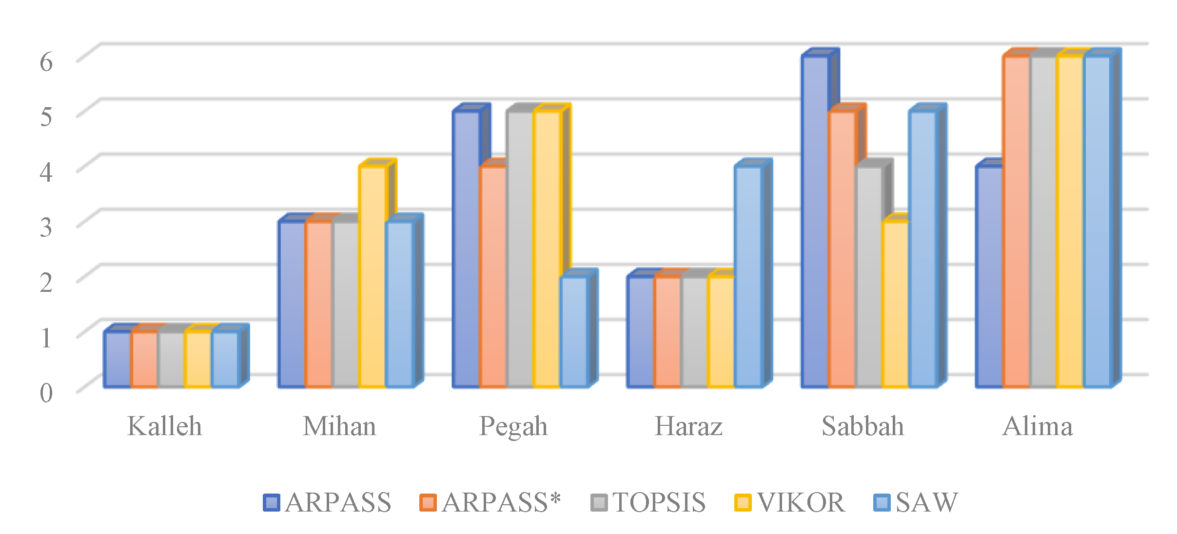
| ARPASS | ARPASS* | TOPSIS | VIKOR | SAW | |
|---|---|---|---|---|---|
| Kalleh | 1 | 1 | 1 | 1 | 1 |
| Mihan | 3 | 3 | 3 | 4 | 3 |
| Pegah | 5 | 4 | 5 | 5 | 2 |
| Haraz | 2 | 2 | 2 | 2 | 4 |
| Damdaran | 7 | 8 | 7 | 7 | 8 |
| Sabbah | 6 | 5 | 4 | 3 | 5 |
| Alima | 4 | 6 | 6 | 6 | 6 |
| Gela | 8 | 7 | 9 | 8 | 7 |
| Domino | 9 | 9 | 8 | 9 | 9 |
| ARPASS | ARPASS* | TOPSIS | VIKOR | SAW | |
|---|---|---|---|---|---|
| Kalleh | 1 | 1 | 1 | 1 | 1 |
| Mihan | 3 | 3 | 3 | 4 | 3 |
| Pegah | 5 | 4 | 5 | 5 | 2 |
| Haraz | 2 | 2 | 2 | 2 | 4 |
| Sabbah | 6 | 5 | 4 | 3 | 5 |
| Alima | 4 | 6 | 6 | 6 | 6 |
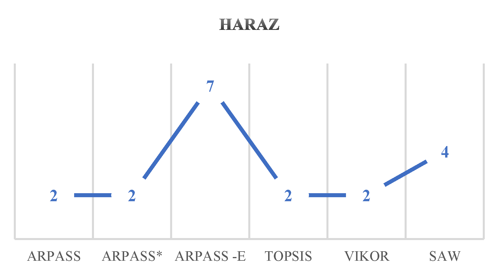
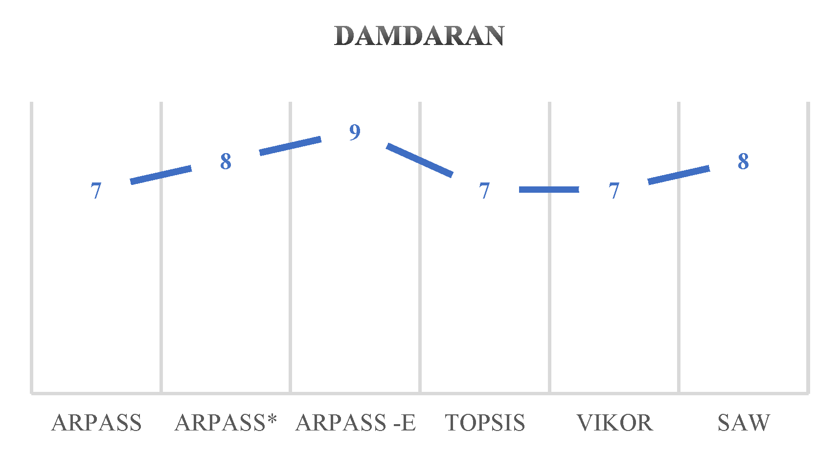
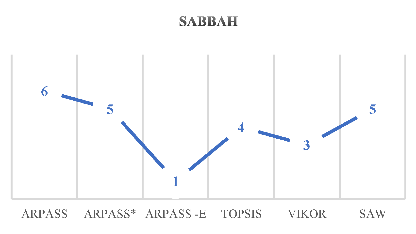
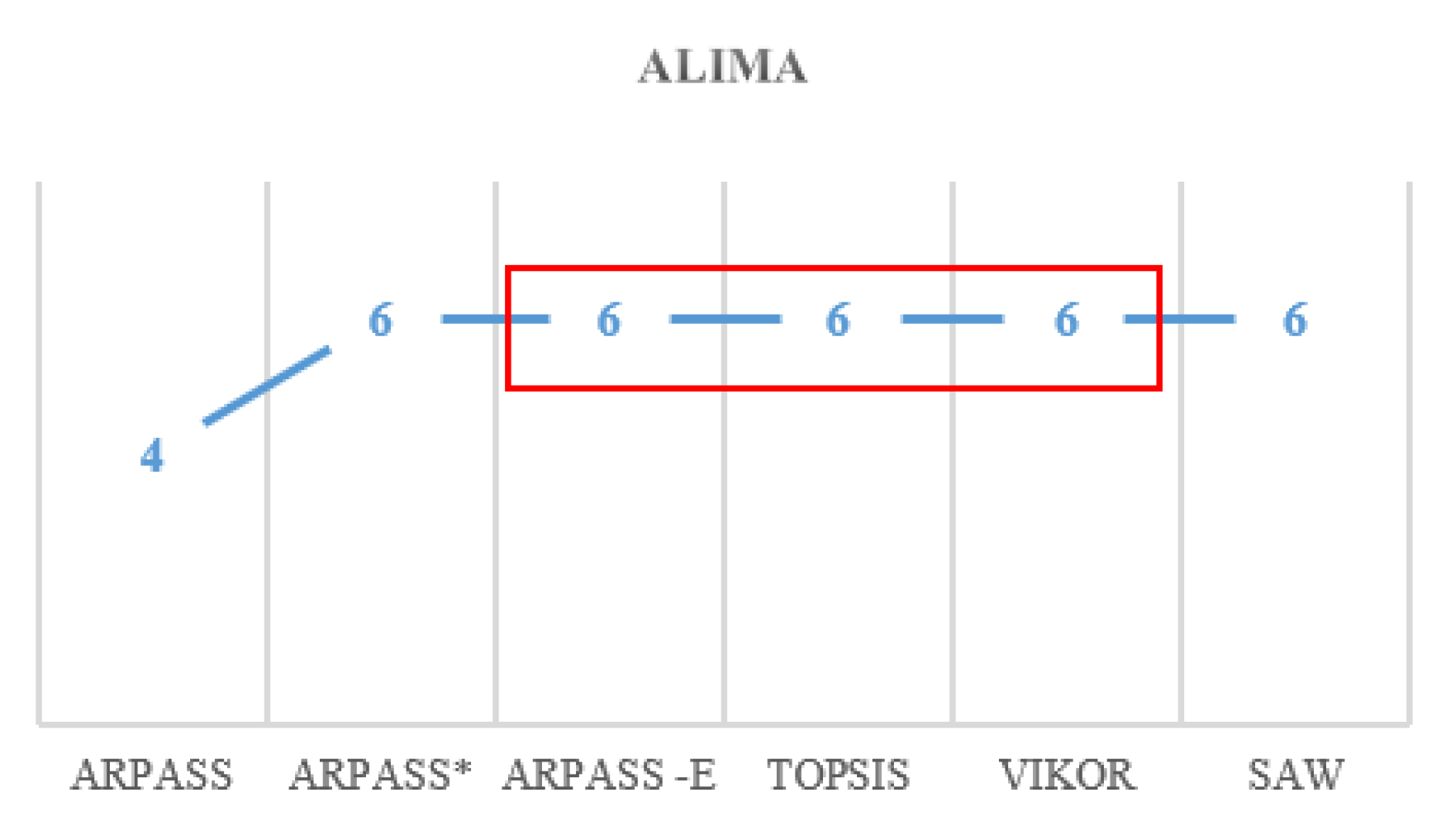
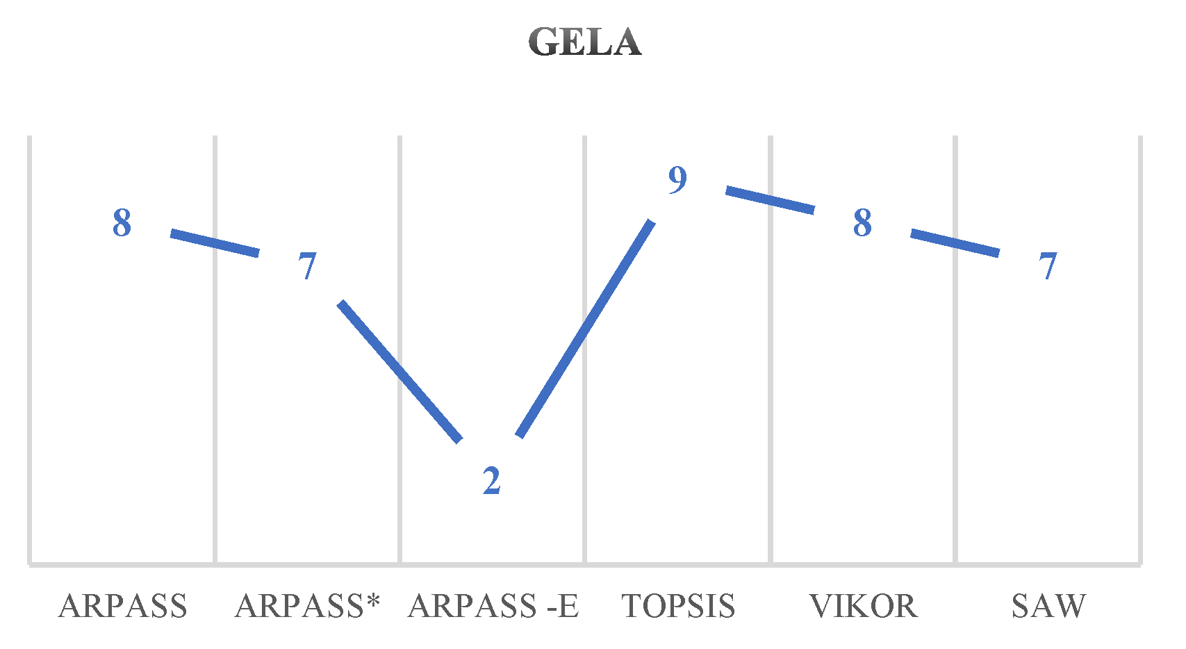
| ARPASS | ARPASS* | ARPASS -E | TOPSIS | VIKOR | SAW | |
|---|---|---|---|---|---|---|
| Kalleh | 1 | 1 | 3 | 1 | 1 | 1 |
| Mihan | 3 | 3 | 4 | 3 | 4 | 3 |
| Pegah | 5 | 4 | 5 | 5 | 5 | 2 |
| Haraz | 2 | 2 | 7 | 2 | 2 | 4 |
| Damdaran | 7 | 8 | 9 | 7 | 7 | 8 |
| Sabbah | 6 | 5 | 1 | 4 | 3 | 5 |
| Alima | 4 | 6 | 6 | 6 | 6 | 6 |
| Gela | 8 | 7 | 2 | 9 | 8 | 7 |
| Domino | 9 | 9 | 8 | 8 | 9 | 9 |
Publisher’s Note: MDPI stays neutral with regard to jurisdictional claims in published maps and institutional affiliations. |
© 2022 by the authors. Licensee MDPI, Basel, Switzerland. This article is an open access article distributed under the terms and conditions of the Creative Commons Attribution (CC BY) license (https://creativecommons.org/licenses/by/4.0/).
Share and Cite
Zakeri, S.; Yang, Y.; Konstantas, D. A Supplier Selection Model Using Alternative Ranking Process by Alternatives’ Stability Scores and the Grey Equilibrium Product. Processes 2022, 10, 917. https://doi.org/10.3390/pr10050917
Zakeri S, Yang Y, Konstantas D. A Supplier Selection Model Using Alternative Ranking Process by Alternatives’ Stability Scores and the Grey Equilibrium Product. Processes. 2022; 10(5):917. https://doi.org/10.3390/pr10050917
Chicago/Turabian StyleZakeri, Shervin, Yingjie Yang, and Dimitri Konstantas. 2022. "A Supplier Selection Model Using Alternative Ranking Process by Alternatives’ Stability Scores and the Grey Equilibrium Product" Processes 10, no. 5: 917. https://doi.org/10.3390/pr10050917
APA StyleZakeri, S., Yang, Y., & Konstantas, D. (2022). A Supplier Selection Model Using Alternative Ranking Process by Alternatives’ Stability Scores and the Grey Equilibrium Product. Processes, 10(5), 917. https://doi.org/10.3390/pr10050917