Investigation of a Novel Deep Borehole Heat Exchanger for Building Heating and Cooling with Particular Reference to Heat Extraction and Storage

Zhang, Jiaqi; Lu, Xinli; Zhang, Wei; Liu, Jiali; Yue, Wen; Ma, Feng

doi:10.3390/pr10050888

Open AccessArticle

Investigation of a Novel Deep Borehole Heat Exchanger for Building Heating and Cooling with Particular Reference to Heat Extraction and Storage

¹

Tianjin Geothermal Research and Training Center, College of Mechanical Engineering, Tianjin University, Tianjin 300350, China

²

Key Laboratory of Efficient Utilization of Low and Medium Grade Energy, MOE, College of Mechanical Engineering, Tianjin University, Tianjin 300350, China

³

Institute of Hydrogeology and Environmental Geology, Chinese Academy of Geological Sciences, Shijiazhuang 050061, China

^*

Authors to whom correspondence should be addressed.

Processes 2022, 10(5), 888; https://doi.org/10.3390/pr10050888

Submission received: 23 March 2022 / Revised: 25 April 2022 / Accepted: 27 April 2022 / Published: 29 April 2022

(This article belongs to the Special Issue Development, Analysis and Optimization of Sustainable Thermal Energy Systems and Technologies)

Download

Browse Figures

Versions Notes

Abstract

:

Medium-depth and deep geothermal energy has been widely used because of its abundant resources and supply stability. Recently, attention has been given to the closed-loop heat extraction system using a deep borehole heat exchanger (DBHE), which enables geothermal energy to be harnessed almost everywhere. In this study, a check valve is adopted in a DBHE system in which the whole section of the well is used for heat extraction in winter during building heating and the upper part of the well is used for heat injection in summer during building cooling. The influence of injected water flowrates, water inlet temperatures, depths of the check valve and formation of thermal conductivities on the performance of this novel DBHE system has been investigated. It is found that heat injection through the upper part of the well in summer can improve the heat extraction rates to a certain extent during the heating season. In summer, the inlet temperature of water has a great influence on the heat injection rates. The increase in the depth of the check valve improves the heat injection rates of the novel DBHE system. When the depth of the check valve is 900 m, the heat injection rates in summer can reach 51.03 kW, which is 27.55% of the heat extraction rates in winter. In this case, the heat injection in summer has the greatest effect on the improvement of heat extraction in winter, which is 6.05 kW, accounting for 3.38% of the heat extraction in that year. It is found that the thermal conductivity of the formation has a great influence on the heat extraction rates in winter and heat injection rates in summer. The proposed novel DBHE system can be used to inject the heat discharged from the building in summer and extract geothermal energy for building heating in winter, forming a better heat balance at certain depths and resulting in a sustainable operation for heating and cooling. Another benefit of using this system is that the heat discharged from air conditioning into the air can be reduced in summer and “urban thermal pollution” can be alleviated.

Keywords:

geothermal energy; deep borehole heat exchanger; heating and cooling; heat injection and storage

1. Introduction

At present, the international energy situation is becoming increasingly grim, the energy consumption structure is in urgent need of transformation, and renewable energy has gradually attracted attention and favor. Geothermal energy has great development potential and prospects because of its large reserves and good stability. Geothermal energy has been widely used in heating in China, but due to China’s policy of “only taking heat but not water”, DBHE systems have been vigorously developed.

DBHEs adapt the structure of a coaxial heat exchanger, and only one well is needed to obtain geothermal energy. Therefore, geothermal water does not directly contact rocks, avoiding the problems of high cost, corrosion and scaling of EGS systems. The EGS has an engineered geothermal reservoir usually created from hot, dry rock resources. The permeability of the reservoir, increased by hydraulic fracturing and heat transmission fluids (such as water or CO₂), can be used to circulate in the reservoir to extract heat from the hot, dry rock resources. The DBHE system was first proposed by Rybach et al. [1] in 1995. In the following twenty years, many scholars have performed a variety of studies on DBHE systems. Mokhtari et al. [2] studied the influence of the pipe diameter ratio of the inner and outer pipes on the performance of a DBHE system. The results show that a pipe diameter ratio of 0.675 has the lowest pressure drop, which means that the energy consumption of the pump is the smallest. However, a pipe diameter ratio of 0.353 has the greatest thermal efficiency. Iry et al. [3] also performed a similar study on the influence of the pipe diameter ratio on the performance of a DBHE system and came to the same conclusion. Oh et al. [4] optimized the depth, roughness of the pipe and shape of the cross section of the pipe. At the same time, the materials of the pipe and grouting are also researched. He et al. [5] mixed graphene with mud and cement as the filler of a DBHE system, which greatly improved the heat collection performance of the system. Hu et al. [6] researched the influence of the physical properties of water and formation on the heat extraction capacity of a DBHE system. They also simulated the heat extraction performance of the DBHE system for abandoned petroleum wells in the Western Canadian Sedimentary Basin. The results show that abandoned petroleum wells have great heat extraction potential.

Xi’an Jiaotong University has performed much experimental research on DBHE systems. Wang et al. [7] established an experimental system and researched the heat extraction performance of the DBHE system. The results show that the system with an inlet velocity of water between 0.3 and 0.7 m/s has a better heat extraction performance. Cai et al. [8] conducted experimental research on a DBHE system with spacings of 15 and 30 m. The results of Cai et al. show that, at the end of the heating season, the outlet temperature of the heat-extraction water from the wells with a distance of 30 m is 0.05 °C higher than that from the wells with a distance of 15 m. Meanwhile, Cai et al. [9] performed a comparative study of four different daily operation-stop times (8–16, 12–12, 16–8 and 24–0). This can provide a reference for the heating of different buildings. Huang et al. [10] adopted a distributed optical fiber temperature sensor (DOFTS) to specifically reflect the temperature change of formation during the long-term operation of a DBHE system. Dijkshoorn et al. [11] studied the cooling and heating capacity of a 2500-m deep well in the center of Aachen, Germany. After 20 years of operation, the system cannot provide the cooling capacity in summer, but it can still provide water between 25 and 55 °C for heating the building.

At present, research on middle and deep DBHE systems mostly focus on their heat extraction capacity, but there is very little research on energy storage in rocks. Among them, Bär et al. [12] established a coupling system of geothermal energy and solar energy to realize heating and power generation. By heating the water to a temperature greater than 110 °C using solar energy and waste heat from a cogeneration plant and reinjecting the water underground through the DBHE, the heat extraction capacity of the system was improved. Welsch et al. [13] established more than 250 different numerical models and compared the heat storage performance of these models by injecting water with a temperature over 70 °C. The results show that the more geothermal wells, the higher the energy storage efficiency. However, these studies have one thing in common, that is, the inlet temperature of geothermal water is higher than the formation temperature at the bottom of the well during the period of energy storage in summer. Although this can ensure heat storage, it cannot achieve refrigeration in summer. This is because the formation temperature around the bottom of the well is too high. For example, the temperature of a well at a depth of 2000 m is approximately 80 °C, so it is difficult to raise the temperature above 80 °C with a heat pump. Therefore, it has become a difficult problem to realize heating in winter and cooling in summer at the same time.

In this paper, the DBHE system is improved. A check valve is set in the middle of the inner pipe, which can realize geothermal water flowing back to the surface from the middle of the heat exchanger in summer and realize heat storage in the shallow formation. Therefore, the cooling effect in summer can be realized. Through this improvement, the novel DBHE system can realize heating in winter and cooling in summer, and the energy storage in summer can also increase the heat extraction rates in the second winter to maintain the sustainable operation of the system.

2. Model and Methodology

2.1. Model

To research the heat extraction rates and heat injection rates of the novel DBHE system, a model is established and simulated by Fluent. A schematic diagram of the novel system is shown in Figure 1. In this figure, a coaxial heat exchanger is placed in the formation, and a check valve is placed in the middle of the inner pipe. The radius of the formation is 100 m, and the depth of the formation is 2100 m. The radius of the inner pipe is set to 0.05 m, and the radius of the outer pipe is set to 0.085 m. The depth of the outer pipe is set to 2000 m, and the depth of the inner pipe is set to 1998 m. The gap of two meters allows water to flow through. The depth of the check valve is a variable between 500 and 900 m. In winter, geothermal water flows into the novel DBHE system from the outer pipe, the check valve is now closed, and geothermal water can flow to the bottom of the well to absorb heat, as shown in Figure 1a. Water can exchange heat with the formation in the whole well section. In summer, geothermal water flows into the novel DBHE system from the inner pipe, the check valve is now open, and geothermal water flows through the check valve to the outer pipe, as shown in Figure 1b. At this time, water can only exchange heat with the formation in the partial well section (depth from the surface to the check valve). Through this design, heating in winter and cooling in summer can be realized.

According to the schematic diagram of the novel DBHE system, the physical model and boundary condition diagram of this system are established, as shown in Figure 2. The figure is the schematic diagram of the model section, Z is the depth direction. The surface of formation is set as the constant wall temperature boundary condition, the other formation boundaries are set as the heat insulation boundary condition. The wall of the well is set as the coupled boundary condition. The boundary conditions of the check valve and the opening of the inner and outer pipes vary according to the operation modes of the system in winter and summer. The boundary conditions of the novel DBHE system are shown in Table 1.

2.2. Methodology

According to the physical model of the novel DBHE system, the grid of the model is established, as shown in Figure 3. A denser grid is used for the formation around the well; the minimum grid size is 0.01 m, and the width of each next grid increases by 1.2 times. For the DBHE system, the grid is uniform, with a size of 0.01 m. In the depth direction, the grid size is set as 0.5 m considering that the vertical geothermal temperature gradient is only 30 °C/km.

The initial conditions are as follows:

(1): The initial formation temperature profile is determined by the surface temperature and geothermal temperature gradient (30 °C/km);
(2): The initial water temperature in the well is set to be the same as the formation temperature distribution;
(3): The initial pressure of water in the well is set to its hydraulic pressure.

The governing equation of the model is the same as Zhang [14], as shown in Appendix A.

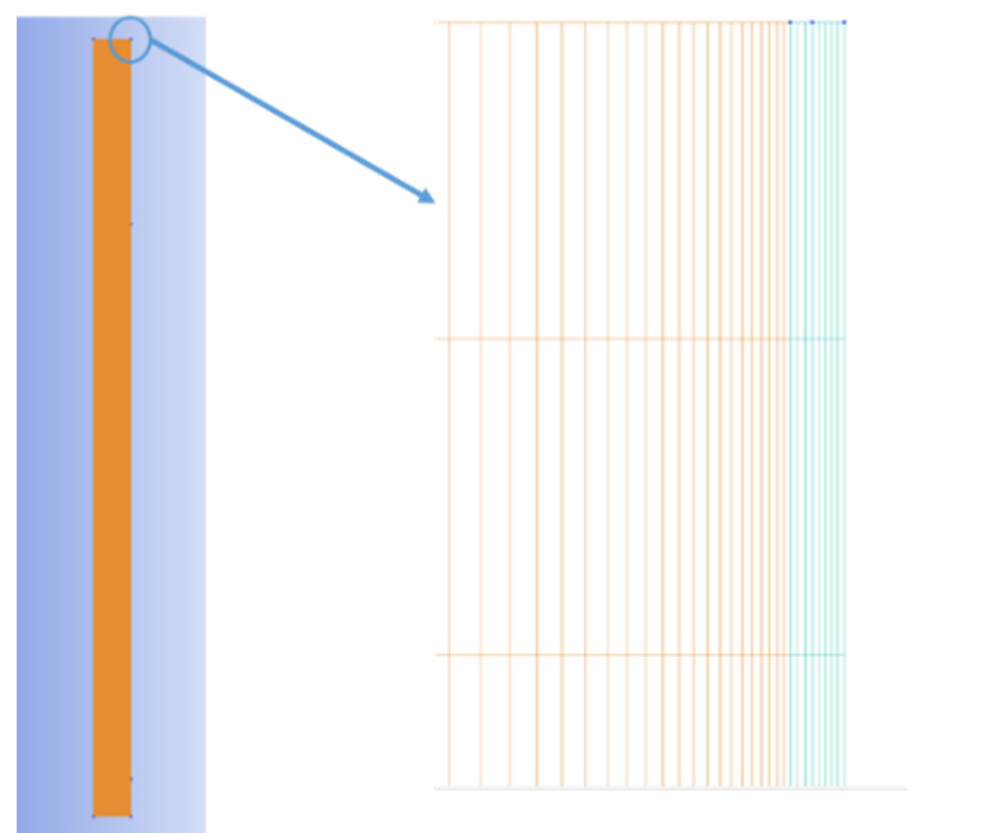
2.3. Model Grid and Time Independence Verification

According to the model of the novel DBHE system, the grid and time step independence are verified by Fluent. The verification of grid independence is divided into two parts: horizontal direction and depth direction. The formation near the wall of the well is densified in the horizontal direction. The minimum grid size of the stratum is 0.01, 0.05, 0.1 and 0.5 m, respectively, and the grid size of the next layer increases by 1.2 times. Formation grid size in the depth direction is evenly divided into 0.1, 0.5, 1 and 2 m. The time steps are set to 60, 600, 3600 and 86,400 s (one day), respectively. The simulation results are shown in Table 2. In the simulation, the inlet temperature of the circulating water is 20 °C, the mass flow is 9 kg/s, the surface temperature is 20 °C and the geothermal gradient is 30 °C/km. Table 2 shows the results of four months of continuous operation of the system.

It can be seen from the table that the minimum grid size of the formation in the horizontal direction has a great impact on the system outlet temperature. The smaller the minimum grid size is, the higher the water outlet temperature is. When the minimum grid size decreases from 0.05 m to 0.01 m, the outlet temperature of the water only increases by 0.03 °C. Therefore, the minimum grid of formation in the horizontal is set as 0.01 m in subsequent simulation calculation. By comparing the grid size in the depth direction, it can be seen that when the grid size changes from 2 m to 0.1 m, the outlet temperature of water does not change. Therefore, the grid size in the depth direction is set to 0.5 m in this paper. By comparing the calculation time step of the model, it is found that when the calculation time step of the model increases from 60 s to 3600 s, the outlet temperature of the water is the same. When the time step increases to 86,400 s, the outlet temperature of the circulating water decreases by 0.01 °C. In order to obtain enough data about the change of water outlet temperature with the system operation time, the time step of the model calculation is set to 3600 s.

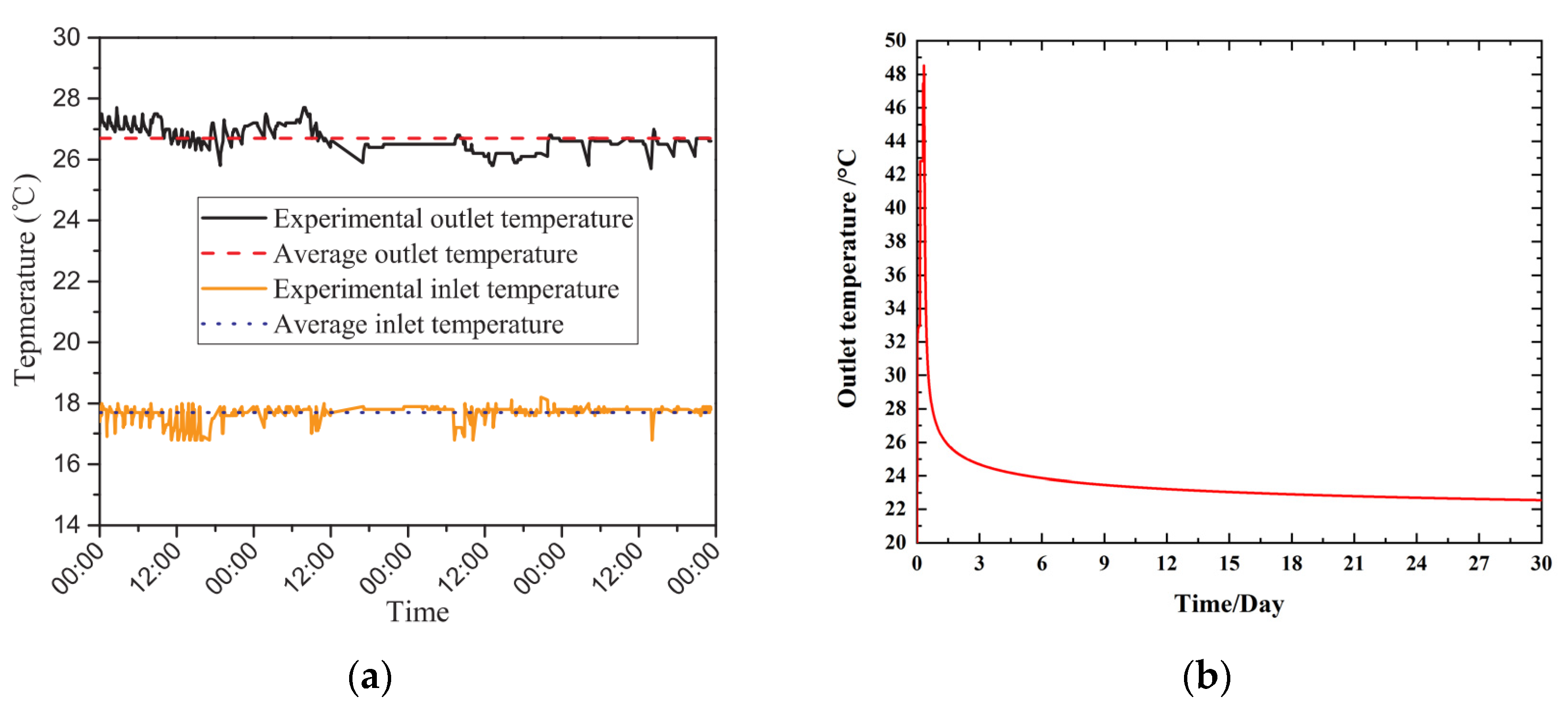
2.4. Model Validation

To verify the accuracy of the model, the results of this model are compared to a demonstration project located in Xi’an. In the demonstration project, a 2000-m coaxial heat exchanger is used to observe the heat extraction of the system. According to the detection of the physical parameters of the formation, the formation is divided into four layers. The specific parameters are shown in Table 3. The specific heat capacity decreases and the thermal conductivity increases with the increase in depth. The inner pipe is 1998 m, and the outer pipe is 2000 m. There is a two-meter gap at the bottom of the well to allow water to flow through. The temperature gradient is 30 °C/km. The temperature of the ground is 15.6 °C. During the test, the average inlet temperature is approximately 17.3 °C, and the average flow is 28 m³/h. The test duration of the demonstration project is one month, and the outlet temperature of the last four days is within the range from 25.4–26.8 °C, as shown in Figure 4a.

Under the same boundary conditions and initial conditions as the demonstration project, Figure 4b shows the outlet temperature of water over one month. It is clear that the outlet temperature of geothermal water drops sharply in the first few days and then tends to level off. The average outlet temperature of the last four days is 22.6 °C. The temperature difference between the demonstration project and simulation results is between 2.8 and 4.2 °C. The main reason is that, in the demonstration project, the specific heat capacity and thermal conductivity of the formation are anisotropic. However, in the simulation, the formation parameters are fixed values, which cannot meet the actual situation. In addition, the inlet temperature and mass flow rate have been changing in the demonstration project, but these two values are fixed values in the simulation Therefore, the temperature difference between the demonstration project and simulation results is considered to be within an acceptable range, and the model is considered to be accurate. Based on this, the heating in winter, cooling in summer and energy storage capacity are researched below.

3. The Performance of the Novel DBHE System under Different Mass Flows

In this section, the heat extraction capacity in winter and the cooling and energy storage capacity in summer of the novel DBHE system under different mass flows and different temperatures of heat injection water are researched.

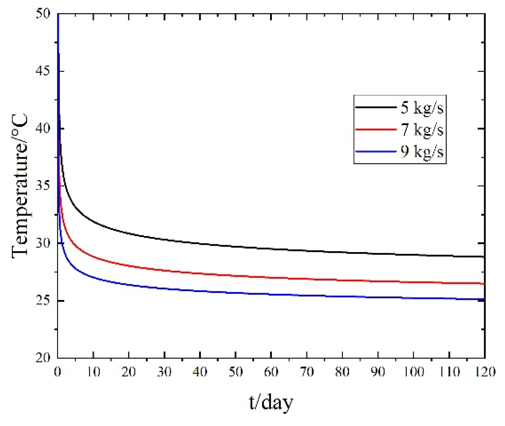
3.1. Heat Extraction Capacity of the Novel DBHE System

To compare the improvement effect of heat injection rates in summer on heat extraction in winter, the heat extraction capacity of the DBHE system for five years under different mass flows is established.

In this section, the heating season is set to four months, and the system will not operate for another eight months. The material of the formation is set to CaCO₃, so the thermal conductivity of the formation is 2.25 W·m⁻¹·K⁻¹. The temperature gradient is set to 30 °C/km. The inlet temperature of geothermal water is set to 20 °C, and the temperature of the ground surface is also set to 20 °C. Figure 5 shows the temperature variation of one heating season under mass flows of 5, 7 and 9 kg/s. In this figure, the outlet temperature decreases with increasing mass flow. Due to the increase in mass flow, the mass of water flowing in unit time increases. Although the mass flow of water increases, the convective heat transfer coefficient between water and formation also increases, the heat exchange between water and formation is greater than the heat conduction of formation. The distant energy of the formation cannot be transmitted to the surrounding well in time and this leads to a small increase in the heat extraction power of water. Under the joint action of the changes in the mass of water and heat extraction power per unit time, the outlet temperature of water decreases with the increase in mass flow.

Table 4 shows the outlet temperature and heat extraction rates under different mass flows over five years. As can be seen, the heat extraction rate of 9 kg/s is the greatest. It is clear that the outlet temperature decreases only slightly. Over five years, the outlet temperature difference between the first and fifth years is 0.64 °C for 5 kg/s. For 7 and 9 kg/s, this value becomes 0.48 and 0.39 °C, respectively. The heat extraction rates of the fifth year decreases approximately 13.44 kW and 7.3% compared to that of the first year. For 7 and 9 kg/s, the values change to 14.11 kW, 14.72 kW, 7.4% and 7.6%, respectively. The greatest heat extraction rates have the greatest percentage of reduction.

Figure 6 shows the temperature change in the formation near the well during the non-heating season. In this figure, the mass flow is 5 kg/s. In one year, the heating season is set to four months, and the non-heating season is set to eight months. This figure demonstrates the monthly temperature change. The 0 month in this figure represents the formation temperature at the end of the heating season, and the months from 1–8 represent the eight months of the non-heating season. In Figure 4, the location of the line is 0.1 m from the outer pipe of the well, and the depth is within the range from 0 to 2000 m. As can be seen, the formation temperature has a great recovery at the end of the first month; the formation temperature recovers to approximately 70 °C at the depth of 2000 m. Then, the temperature recovery effect of each month gradually weakens. At the end of the eighth month, the formation temperature recovers to approximately 77 °C at the depth of 2000 m.

Table 5 shows the temperature recovery effect of 5, 7 and 9 kg/s month by month. In this table, temperatures at depths of 1000 and 1998 m are listed. The reason for choosing 1998 m instead of 2000 m is that the length of the inner pipe is 1998 m and the length of the outer pipe is 2000 m. When the geothermal water flows from the outer pipe into the inner pipe, it basically flows near a depth of 1998 m. The water at 2000 m basically does not flow. Therefore, observing the temperature change at a depth of 1998 m can better reflect the temperature change. From the table, the temperature recovery effect in the first month is the best, and the temperature recovery effect after the second month is very small. Although the heat extraction rates of different mass flows has a difference, the temperature of the formation of different mass flows is basically the same after eight months. The formation temperature at a depth of 1000 m recovers to 48.15 °C, and for 1998 m, the temperature recovers to 77.25 °C. The initial temperatures at 1000 and 1998 m are 50 °C and 79.94 °C, respectively. The recovery of the formation temperature to a higher level can ensure that there is little effect in heat extraction rates in the second year. In addition, the formation temperature of 1998 m recovers to approximately 73 °C after two months. This time is when a cooling load is needed in summer. If heat is recharged into the formation from the bottom of the well, the temperature of the water in summer needs to be higher than 73 °C. It is very difficult to raise the temperature above 73 °C with a heat pump system. However, if geothermal water is allowed to recharge heat at depths of 1000 m or less than 1000 m, it is much easier to make the water temperature reach 50 °C. If the depth is shallower, the temperature of geothermal water can be lower. Therefore, the effect of cooling and energy storage in summer is studied.

3.2. Heat Injection Capacity of the Novel DBHE System

In this section, the depth of the check valve is set to 500 m. The initial temperature at 500 m is 35 °C, so the inlet temperature of heat injection water is set to 40, 45 and 50 °C in summer. In addition, the inlet temperature of heat injection water in summer can easily be reached by the heat pump.

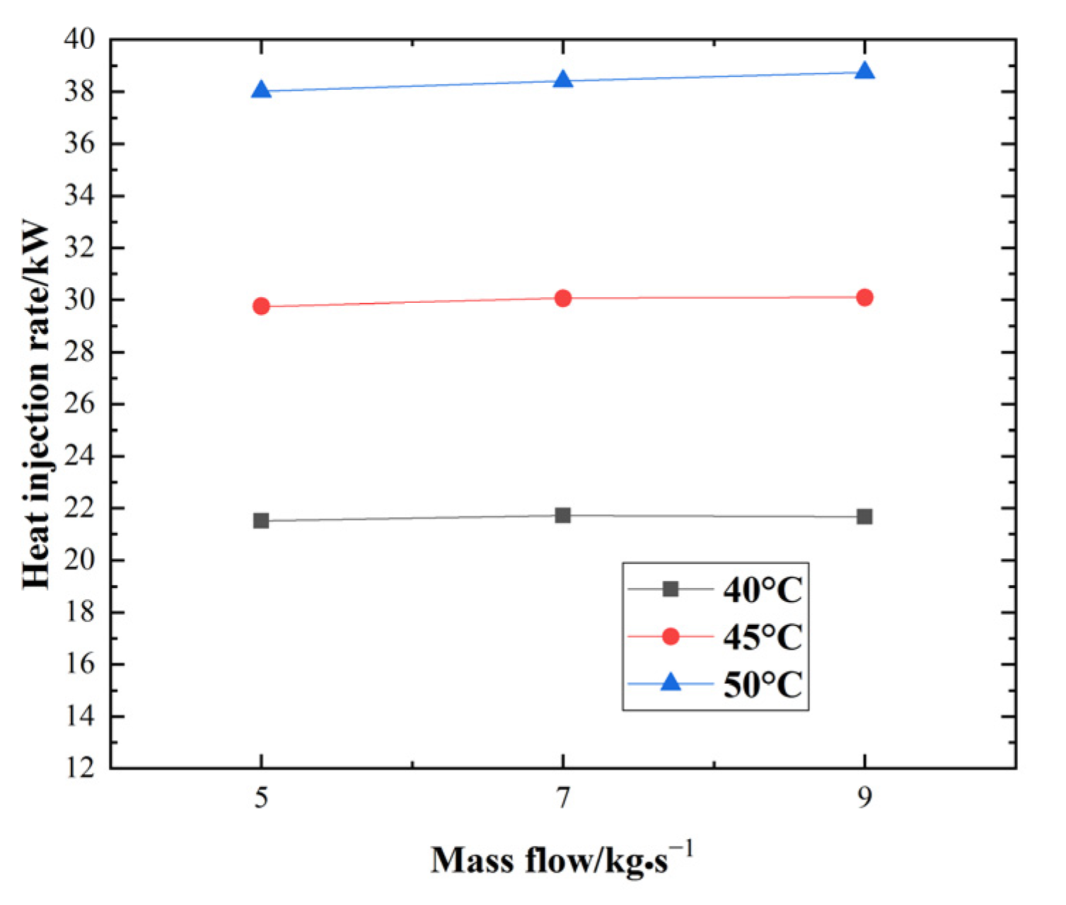
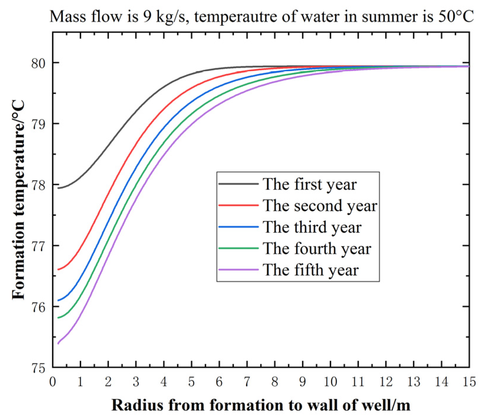
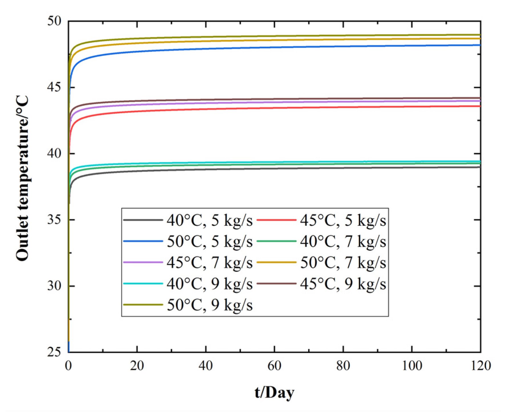
3.2.1. Heat Injection and Energy Storage Capacities of the Novel DBHE System

In this model, the heating season is set to four months, and the cooling season is also set to four months. Between the heating and cooling seasons, the system stops running for two months to recover the temperature of the formation.

After four months of heating and two months of non-operation, there was four months of cooling. The outlet temperature of water under different mass flows and different inlet temperatures of heat injection water in summer is shown in Figure 7. As can be seen, the outlet temperature changes greatly in the first days and then remains basically the same. With the increase in the inlet temperature, the temperature difference between the inlet and outlet increases. This is because the temperature of the formation is the same for every case, and the temperature difference between the inlet temperature and formation increases with increasing inlet temperature. After operation of the system, the formation temperature around the well rises rapidly. However, the heat transfer from the formation around the well to the distance is very slow, so the heat transferred from the water cannot diffuse rapidly; thus, the outlet temperature of the water is kept at a high level.

Figure 8 shows the heat injection rates under different mass flows and different inlet temperatures of water in summer. In this figure, the inlet temperature of water in summer has a decisive influence on the heat injection rates, but the mass flow has little effect on it. There are two reasons: (1). When the mass flow increases, and the convective heat transfer coefficient increases accordingly, it leads to the increase in heat injection rates of the system; (2). When the check valve is opened in summer, a small amount of water flows to the bottom of the well. Due to the high formation temperature at the bottom of the well, this part of the water will absorb a small amount of heat, thus, reducing the heat injection rates of the system. The greater the mass flow, the more water flows to the bottom of the well. Under the joint action of the above two points, the mass flow has no effect on the heat injection rates in summer.

Table 6 shows the annual heat injection rates over five years. In this table, the heat injection rate is the greatest based on 9 kg/s and 50 °C; compared with the first year, the heat injection rate decreased by 1.77 kW in the fifth year, accounting for 4.57%. The heat injection rate is the minimum based on 5 kg/s and 40 °C, compared with the first year, the heat injection rate decreased by 0.76 kW in the fifth year, accounting for 4%. Compared with the condition that the temperature of heat injection water is 40 °C, when the depth of the check valve is 500 m, using heat injection water with temperatures of 45 °C and 50 °C can increase the heat injection rates by approximately 37% and 75%, respectively.

Figure 9 shows the formation temperature near the well at depths from 0 to 600 m during the non-heating season. All lines in the figure can be divided into four parts.

Part 1: The line of month 0 indicates the formation temperature at the end of the heating season;

Part 2: The lines of month 1 and month 2 indicate the non-operation process between the heating season and cooling season;

Part 3: The lines of months 3–6 indicate the cooling season in summer;

Part 4: The lines of month 7 and month 8 indicate the non-operation process between the cooling season and the next heating season.

In Figure 9, the mass flow is set to 5 kg/s, and the inlet temperature in summer is set to 50 °C. The depth of the check valve is 500 m. In Parts 1 and 2, the formation temperature near the well is the same as that of the system without the cooling season. In Part 3, the formation temperature has changed dramatically because of the heat injection in summer. At a depth of 500 m, the formation temperature near the well is approximately 46 °C at the end of 3 months. After the cooling season, the formation temperature near the well increases to 47 °C. The formation temperature at depths from 0 to 500 m increases greatly. In Part 4, due to the high temperature of the formation around the well, the heat of the formation around the well will be transferred to the distant formation through heat conduction. Therefore, the formation temperature near the well in Part 4 is lower than that in the previous four months in Figure 9. However, the formation temperature at the end of the last month in Figure 9 is higher than that in Figure 6. This will help to improve the heat extraction rates in the next heating season.

Figure 10 shows the change in formation temperature at a depth of 400 m for one year. In this figure, the abscissa is the radius from formation to the wall of the well. At a depth of 400 m, the initial temperature of the formation is 32 °C. In Part 1 (at the end of the heating season), the formation temperature increases with increasing distance from the well. In Part 2, the formation temperature around the well recovers considerably, but the formation temperature decreases over 4 m because the distant formation conducts heat to the formation around the well. In Part 3, the formation temperature becomes very high because the inlet temperature of the water is 50 °C in the cooling season. The heat is transferred to the formation through the water. Therefore, in Part 3, the formation temperature increases every month. In Part 4 (non-operation), because of the high temperature of the formation around the well, the heat conducts heat from the formation around the well to the distant formation. As can be seen, the formation temperature at 8 months is higher than the initial temperature of formation (32 °C).

3.2.2. Influence of Heat Storage on the Heat Extraction Capacity in Winter

The cooling season of the novel DBHE system can increase the formation temperature at the depth from the surface to the check valve. This performance can improve the heat extraction rates in the next heating season. Table 7 shows the heat extraction rates over five years under different mass flows and different summer inlet temperatures. The heat extraction rates of the novel DBHE system under the same mass flow are the same for the first year. This is because the system is calculated from the heating season. The influence of the heat injection in summer on the heat extraction in winter begins to appear in the second year. By comparing Table 4 and Table 7, it can be found that cooling in summer can increase the heat extraction rates in winter. Different inlet temperatures in summer have different effects on increasing heat extraction rates. For the mass flow of 5 kg/s, the differences in the heat extraction rates are 1.17, 1.74, 1.97 and 2.26 kW for the second to fifth years under an inlet temperature of 40 °C. For an inlet temperature of 45 °C and 50 °C, the values change to between 1.58 and 2.95 kW and 1.98 and 3.64 kW. For the mass flow of 7 kg/s, the different heat extraction rates are from 1.33–2.25 kW, 1.78–3.00 kW and 2.22–3.60 kW, respectively, under the inlet temperature of 40 °C, 45 °C and 50 °C. For the mass flow of 9 kg/s, the different heat extraction rates are from 1.69–2.58 kW, 2.16–3.36 kW and 2.60–4.18 kW, respectively, under the inlet temperature of 40 °C, 45 °C and 50 °C. Under the same inlet temperature of water, the influence of the mass flow changes on the difference in the heat extraction rates is negligible, and the influence of the inlet temperature of water changes on the difference in the heat extraction rates is greater.

Figure 11 shows the temperature change in the formation temperature at 1998 m over five years. In the figure, the mass flow is 9 kg/s and the inlet temperature of the water in summer is 50 °C. It can be seen from the figure that the temperature of the formation gradually decreases with the increase in operation years due to the heat extraction from the formation. At the end of the first year, the temperature of the formation around the well is close to 78 °C. At the end of the fifth year, the temperature of the formation around the well is approximately 75.4 °C. The influence radius of the system on the temperature of formation also increased from 20 m in the first year to nearly 50 m in the fifth year.

4. Performance of the Novel DBHE System under Different Check Valve Depths

In this article, a novel DBHE system with check valve depths of 500 m, 700 m and 900 m is researched. The initial temperature of the formation at a depth of 700 m is 41 °C, and the initial temperature of the formation at a depth of 900 m is 47 °C. The heat extraction rates and heat injection rates of the novel DBHE are observed based on a mass flow of 9 kg/s. The inlet temperature of heat injection water in summer is also set to 40, 45 and 50 °C.

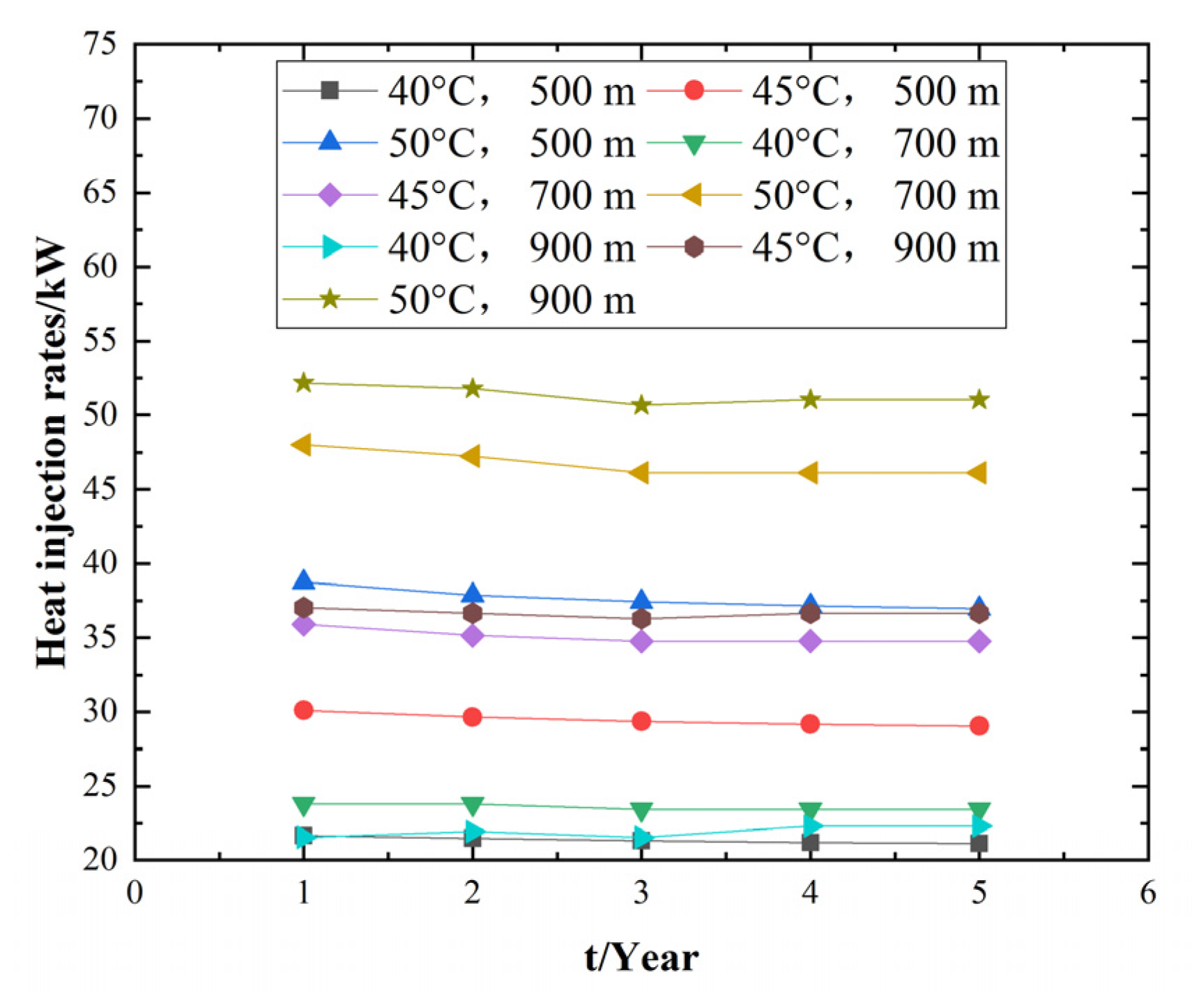
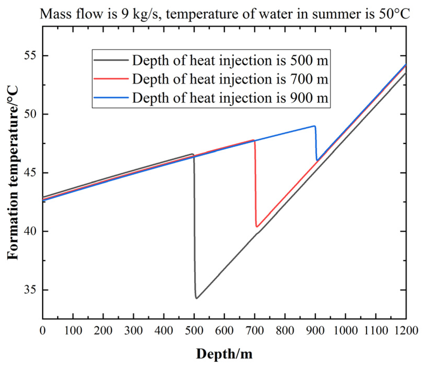
4.1. Heat Injection Capacity of the Novel DBHE System under Different Check Valve Depths

Figure 12 shows the heat injection rates of different depths of the check valve. The range of heat injection rates is between 21 and 52 kW. As can be seen, the novel DBHE system in which the check valve has a depth of 900 m and the heat injection water has an inlet temperature of 50 °C in summer (hereafter referred to as depth and temperature, such as “900 m and 50 °C”) has the greatest heat injection rates. The minimum heat injection rate is the case of 500 m and 40 °C. The following two situations also need attention: (1). The heat injection rates of 700 m and 50 °C are higher than those of 900 m and 45 °C; (2). The heat injection rates of 900 m and 40 °C are very small. The reason is that the initial temperature of formation is 47 °C. After the heating season and two months of the nonoperation season, the formation temperature near the well at a depth of 900 m is 42.95 °C. When the inlet temperature of water is set to 40 °C in summer, the energy is transferred from the formation around the well to the water. This process has a negative effect on the heat injection rates in summer. Energy cannot be transferred to the formation from the water until the temperature of the water is higher than the temperature of the formation around the well. Therefore, the heat injection rates of 900 m and 40 °C are smaller than those of most cases. Compared with the condition that the temperature of heat injection water is 40 °C, when the depth of the check valve is 900 m, using heat injection water with temperatures of 45 °C and 50 °C can increase the heat injection rates by approximately 65% and 130%, respectively.

Figure 13 shows the temperature change in the formation with a check valve depth of 500 m, 700 m and 900 m. It can be seen from the figure that the heat injection of the system in summer only affects the temperature of the formation from the surface to the depth of the check valve. When the depth of the check valve is 500 m, the temperature of the formation drops sharply at 500 m. The same phenomenon exists when the depth of the check valve is 700 m and 900 m. At the same time, when the depth of the check valve is 500 m, the temperature of formation within 0–500 m is higher than that of 700 m and 900 m. This is because, under the same mass flow and water inlet temperature, the temperature of formation with a depth of 500 m is lower than 700 m and 900 m. In the process of water flowing upward from 900 m, the temperature of water gradually decreases. Therefore, the temperature difference between the formation and the water at the depth of 500 m is large, and the heat exchange rates are also large. As a result, the temperature of formation with a depth of 500 m is higher than the other two working conditions.

4.2. Heat Extraction Capacity of the Novel DBHE System under Different Check Valve Depths

Table 8 shows the heat extraction rates of different depths of the check valve. Since the novel DBHE system is calculated from the heating season, the heat extraction rate of each case is equal in the first year. After heat injection in summer, the heat extraction rate of each case begins to change. The novel DBHE system with 900 m and 50 °C has the greatest heat extraction rates. The order of heat extraction rates in other cases is the same as that of the heat injection rates in summer. The reason is that the heat injection rates in summer play a positive role in the increase in heat extraction rates in winter. The greater the heat injection rates in summer, the greater the heat extraction rates in winter. By comparing the DBHE system with and without cooling in summer in the case of 900 m and 50 °C, it can be calculated that the increases in the heat extraction rate are 3.40, 6.05, 5.29 and 6.05 kW from the second to the fifth year. This is equivalent to increases of 1.82%, 3.30%, 2.92% and 3.38%.

By comparing the heat extraction rates and heat injection rates of the novel DBHE system, the heat injection rate in summer is 27.55% of the heat extraction rate in winter at the fifth year for the case of 900 m and 50 °C. For the other cases, the percentage is much smaller.

5. Performance of the Novel DBHE System under Different Thermal Conductivities of Formation

For the DBHE system, the thermal conductivity of the formation is a very important factor affecting the heat extraction capacity of the system. In the above research, the thermal conductivity of the formation is set to 2.25 W/m·K. In this part, thermal conductivities of 1.25 and 3.25 W/m·K are also studied. The inlet temperature of the water is set to 20 °C in winter and 40, 45, and 50 °C in summer. The mass flow of water is set to 9 kg/s. Based on different thermal conductivities of formation, the heat injection capacity of the novel DBHE system in summer is researched.

Figure 14 shows the influence of the thermal conductivity of the formation on the heat extraction rates of the novel DBHE system. For the thermal conductivity of 1.25 W/m·K, the heat extraction rates decrease from 118.6 to 108.5 kW within five years. For 2.25 W/m·K⁻¹ and 3.25 W/m·K, the values change to between 193.9 and 179.2 and 262.7 and 244.2 kW, respectively.

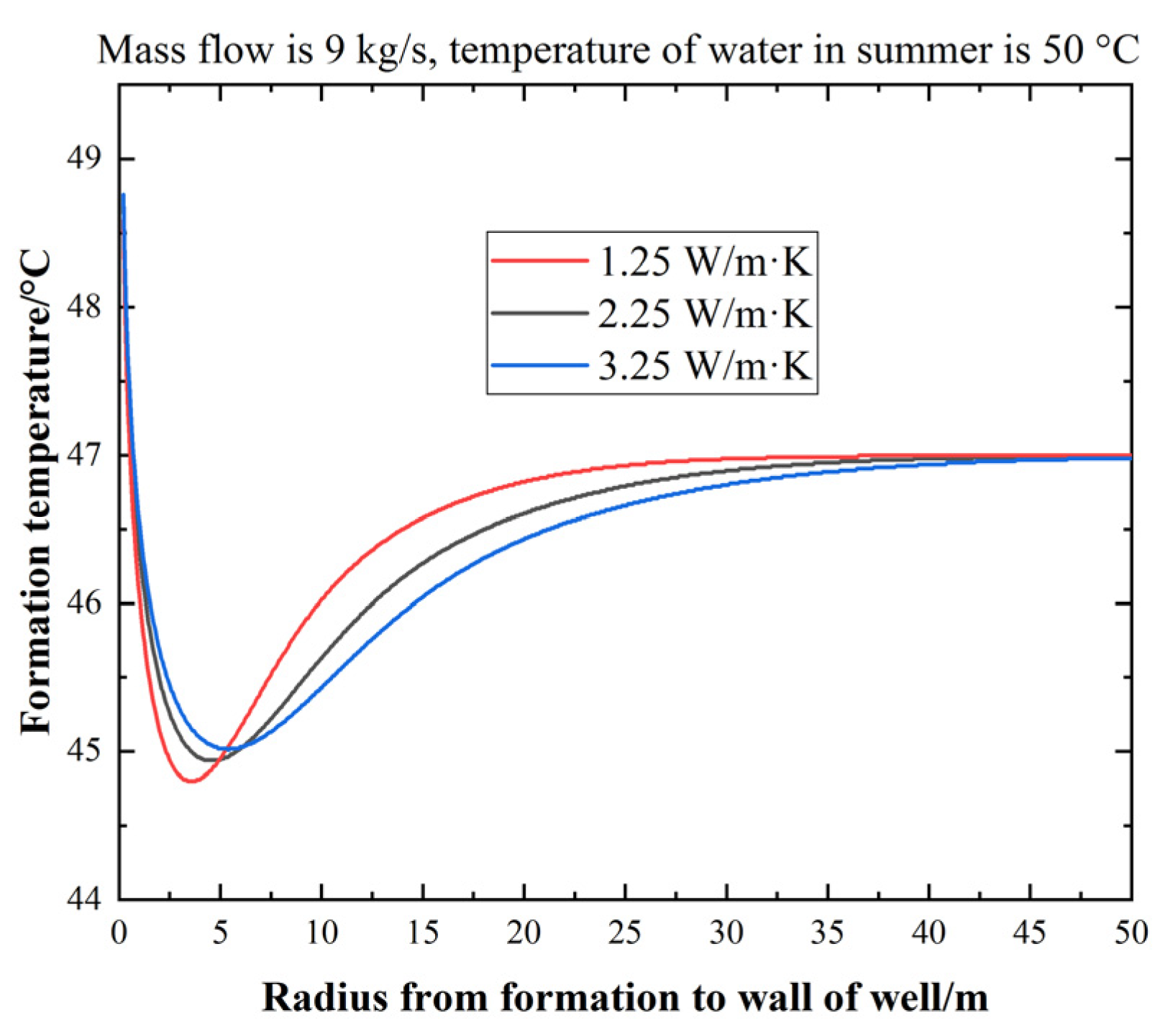
5.1. Heat Injection Rates of the Novel DBHE System under Different Thermal Conductivities

Figure 15 shows the heat injection rates of the novel DBHE system under different thermal conductivities. A greater thermal conductivity has greater heat injection rates under the same inlet temperature of heat injection water in summer. The trend is the same as that of the heat extraction rates in winter. In this figure, the maximum heat injection rate is approximately 70 kW for a thermal conductivity of 3.25 W/m·K and an inlet temperature of 50 °C. The heat injection rate in summer is 27.72% of the heat extraction rate in winter. The minimum heat injection rate is approximately 13 kW for a thermal conductivity of 1.25 W/m·K and an inlet temperature of 40 °C. The heat injection rate in summer is only approximately 10.86% of the heat extraction rate in winter. The heat injection rate of 2.25 W/m·K and 50 °C is slightly higher than that of 3.25 W/m·K and 40 °C. The heat injection rate is mainly determined by the thermal conductivity of the formation and inlet temperature of water in summer.

Figure 16 shows the effect of the thermal conductivity of the formation on the temperature during energy storage in summer. In the figure, the depth of the check valve is 900 m, the depth of the observed formation is 900 m, the mass flow is 9 kg/s and the inlet temperature of the water in summer is 50 °C. It can be seen from the figure that at the end of heat injection in the fifth year, the influence radius of the formation temperature around the well corresponding to the three thermal conductivity coefficients is basically the same. With the increase in the distance between the formation and the wall of the well, the influence of thermal conductivity on the temperature of the formation increases gradually. In the figure, the smaller the thermal conductivity of the formation, the smaller the minimum temperature at 900 m. This is because the smaller the thermal conductivity, the harder it is to transfer the heat of the formation around the well and the heat of the remote formation to the lowest point. The thermal conductivity of formation also has a great influence on the influence radius of the system. The influence radius of the system with thermal conductivity of 1.25 W/m·K is only approximately 30 m, and the influence radius of the system with thermal conductivity of 3.25 W/m·K is approximately 50 m.

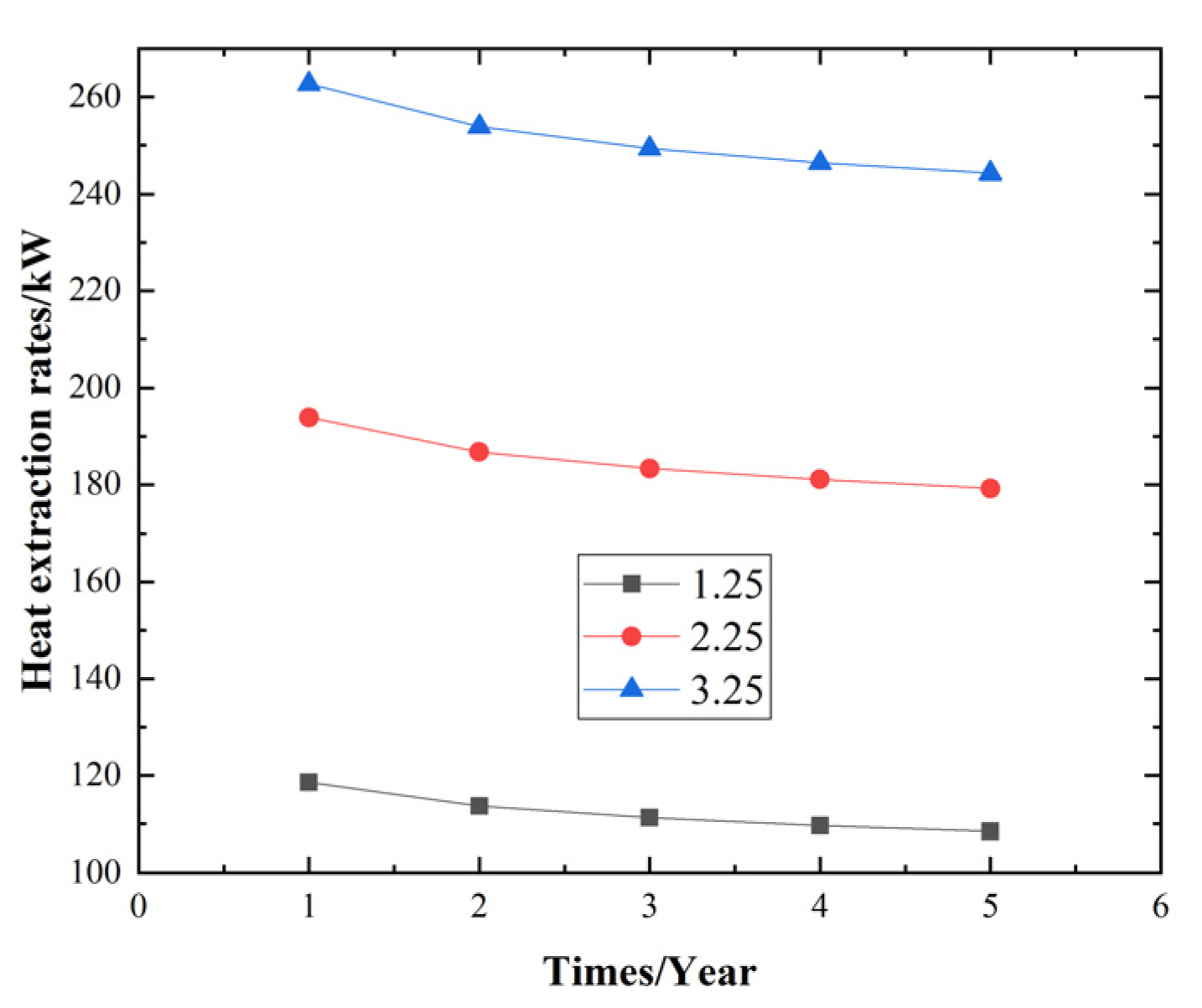
5.2. Heat Extraction Capacity of the Novel DBHE System under Different Thermal Conductivities of Formation

When the novel DBHE system realizes both heating in winter and cooling in summer, the heat extraction rates of the novel DBHE change. Table 9 shows the heat extraction rates of the novel DBHE system with inlet temperatures of 40, 45 and 50 °C in summer. In the first year, the system with the same thermal conductivity has the same heat extraction rates. This is because the model is calculated from the heating in winter, and the impact of cooling in summer will not appear until the next heating season. At the end of the heating season of the fifth year, the heat extraction rates increase by 1.94, 3.04 and 3.17 kW for thermal conductivities of 1.25, 2.25 and 3.25 kW, respectively, based on an inlet water temperature of 40 °C. When the inlet temperature of water changes to 45 and 50 °C, the heat extraction rates increase from 1–2 kW, respectively. In terms of the percentage increase in heat extraction rates, the lower thermal conductivity (1.25 W/m·K) has the greatest value (3.61%) because it has the minimum heat extraction rates. For thermal conductivities of 2.25 and 3.25 W/m·K, the values change to 3.38% and 2.74%, respectively. The heat injection rate in summer is 27.72% of the heat extraction rate in winter in the fifth year for the case of 3.25 W/m·K and 50 °C.

6. Conclusions

In this investigation, a check valve is adopted in a DBHE system in which the whole section of the well is used for heat extraction in winter during building heating and the upper part of the well is used for heat injection in summer during building cooling. The influence of injected water flowrates, water inlet temperatures, depths of the check valve and the formation of thermal conductivities on the performance of this novel DBHE system has been studied numerically. It has been found that the novel DBHE system can be used to inject and store heat at depth, maintain the heat balance there and realize sustainable operation for heating and cooling. Furthermore, using this system can reduce the heat emission into the air in summer and, hence, alleviate urban thermal pollution. Based on the analysis of the simulation results, the following conclusions can be drawn from this study:

(1): The novel DBHE system can realize injecting and storing heat in the formation in summer and improve the heat extraction rates in the next heating season;
(2): The inlet temperature of the injected water in summer has a great influence on the heat injection rates of the novel DBHE system. The higher the inlet temperature, the greater the heat injection rates. Compared with the condition that the temperature of heat injection water is 40 °C, when the depth of the check valve is 500 m, using heat injection water with temperatures of 45 °C and 50 °C can increase the heat injection rates by approximately 37% and 75%, respectively; the heat injection rates can increase to 65% and 130% if the depth of the check valve is 900 m;
(3): The increase in the depth of the check valve improves the heat injection rates of the novel DBHE system. When the depth of the check valve is 900 m and the inlet temperature is 50 °C, the heat injection rate can reach 51.03 kW, which is 27.55% of the heat extraction rate in winter for the fifth year. In this case, the heat injection in summer has the greatest effect on the improvement of heat extraction in winter, which is 6.05 kW, accounting for 3.38% of the heat extraction in that year;
(4): The thermal conductivity of the formation has a great influence on the heat extraction rates in winter and heat injection rates in summer. The higher the thermal conductivity, the greater the heat extraction and injection rates. When the thermal conductivity is 1.25 W/m K, the heat injection rate in summer is 31.14 kW, which is 10.86% of the heat extraction rate in winter. When the thermal conductivity is 3.25 W/m K, the heat injection rate in summer is 69.55 kW, and the percentage changes to 27.72%.

Author Contributions

J.Z., X.L. and W.Z. participated in the study concept, model and review of the manuscript; J.Z., J.L. and W.Y. participated in the model calculations; F.M. participated in the review of the manuscript. All authors have read and agreed to the published version of the manuscript.

Funding

This research was funded by the Ministry of Science and Technology: 2019YFB1504105.

Institutional Review Board Statement

Not applicable.

Informed Consent Statement

Not applicable.

Data Availability Statement

Not applicable.

Acknowledgments

The authors gratefully acknowledge the financial support provided by the National Key Research and Development Program of the 13th Five-Year Plan of China (No. 2019YFB1504105).

Conflicts of Interest

The authors declare no conflict of interest.

Appendix A. DBHE Model

The governing equations of DBHE in this study are shown below.

Continuity equation:

\frac{\partial}{\partial t} (ρ) = - \frac{\partial}{\partial z} (ρ v) + m

(A1)

where

ρ

is the density of water, kg/m³;

v

is the velocity of the water, which is the rate of volume flow across the cross-sectional area of the annular or the inner pipe in this 1D equation, m/s;

m

is the mass sink/source term, kg/m³·s.

Momentum equation:

\frac{\partial P}{\partial z} = ρ g \cos (θ) \pm \frac{f ρ v^{2}}{2 d} \pm (\frac{\partial}{\partial t} (ρ v) + \frac{\partial}{\partial z} (ρ v^{2}))

(A2)

where

P

is the fluid pressure, Pa;

g

is the gravitational acceleration, m/s²;

θ

is the inclination of the well;

f

is the fraction factor;

d

is the wellbore hydraulic diameter, m.

Energy equation:

\frac{\partial}{\partial t} (ρ (h - \frac{P}{ρ} + \frac{v^{2}}{2})) = - \frac{\partial}{\partial z} (ρ v (h + \frac{v^{2}}{2})) - ρ v g \cos (θ) - \frac{q}{A} + Q

(A3)

where

h

is the enthalpy of water, kJ/kg;

q

is the lateral heat flow gradient, W/m;

Q

is the heat sink/source term, W/m³. In the formula, z is the coordinate in the vertical direction.

For the inner pipe fluid, the heat flow is calculated by:

q = q_{1} = A_{1} U (T_{1} - T_{2})

(A4)

where

q_{1}

is the heat exchange rate between the inner pipe flow and the annular flow, W;

U

is the overall heat transfer coefficient between the inner pipe flow and annular flow, W/(m²·K);

A_{1}

is the heat exchange area of the inner pipe inside surface, m²;

T_{1}

is water temperature of the inner pipe flow, K;

T_{2}

is the water temperature of the annular flow, K.

U A_{1} = \frac{π}{\frac{1}{2 a_{1} r_{1}} + \frac{1}{2 λ_{1}} \ln \frac{r_{2}}{r_{1}} + \frac{1}{2 a_{2} r_{2}}}

(A5)

where

a_{1}

is the convective heat transfer coefficient corresponding to the inner pipe flow, W/(m²·K);

r_{1}

is the inner radius of the inner pipe, m;

λ_{1}

is the thermal conductivity of the inner pipe material, W/(m·K);

a_{2}

is the convective heat transfer coefficient corresponding to the annular flow associated with the outer wall of the inner pipe, W/(m²·K);

r_{2}

is the outer radius of the inner pipe, m.

For the annular pipe fluid, the heat flow is calculated by:

q = q_{2} + q_{1}

(A6)

q_{2} = 2 π r_{3} a_{3} (T_{3} - T_{2})

(A7)

where

q_{2}

is heat exchange rate between the outer pipe and rock, kW;

a_{3}

is the convective heat transfer coefficient corresponding to the annular flow associated with the inner wall of the outer pipe, W/(m²·K);

r_{3}

is inner radius of the annular pipe, m;

T_{3}

is the temperature of the outer pipe wall, K.

In this model, the energy conservation equation of the geological formation around the well is as follows:

\frac{\partial T_{fm}}{\partial t} = \frac{1}{ρ_{fm} C_{fm}} (\frac{1}{r} \frac{\partial}{\partial r} (λ_{fm} r \frac{\partial T}{\partial r}) + \frac{\partial}{\partial z} (λ_{fm} \frac{\partial T}{\partial z}))

(A8)

where

T_{fm}

is the temperature of formation, K;

λ_{fm}

is thermal conductivity of the formation, W/(m·K);

ρ_{fm}

is the formation density, kg/m³;

C_{fm}

is the specific heat of the formation, J/(kg·K).

The three convective heat transfer coefficients,

a_{1}

,

a_{2}

and

a_{3}

, can be determined by using the following equations and Table A1:

a = \frac{N u λ}{d}

(A9)

N u = 0.023 R e^{0.8} P r^{n}

(A10)

R e = \frac{ρ v d}{μ}

(A11)

P r = \frac{c_{p} μ}{λ}

(A12)

where

N u

is the Nusselt number; λ is the thermal conductivity of the water, W/(m·K)

d

is the characteristic length, m;

R e

is the Reynolds number;

P r

is the Prandtl number; ρ is the density of the water (kg/m³); v is the volumetric flux of the water, m/s;

μ

is the dynamic viscosity of the water, Ns/m²;

c_{p}

is the specific heat capacity, J/(kg·K). The characteristic length d, the value of n (Index in Equation (A10)), and other relevant parameters are defined in Table A1.

Table A1. Parameters used for determining the convective heat transfer coefficients.

	$a_{1}$	$a_{2}$	$a_{3}$
λ	Thermal conductivity of water in the inner pipe	Thermal conductivity of water in the annular	Thermal conductivity of water in the annular
d	Inner diameter of the inner pipe	Inner diameter of the outer pipe minus outer diameter of the inner pipe	Inner diameter of the outer pipe minus outer diameter of the inner pipe
v	Volumetric flux of water in the inner pipe	Volumetric flux of water in the annular	Volumetric flux of water in the annular
μ	Dynamic viscosity of water in the inner pipe	Dynamic viscosity of water in the annular	Dynamic viscosity of water in the annular
c_p	Specific heat capacity of water in the inner pipe	Specific heat capacity of water in the annular	Specific heat capacity of water in the annular
n (Index in Equation (A10))	0.3	0.4	0.4

In this study, the governing equations are solved in the following way:

For a given time-step, pressure field, and other initial and boundary conditions, the discrete momentum equation is solved to obtain a velocity field.

The relationship between the pressure and velocity specified by the discrete momentum equation is brought into the discrete continuity equation to obtain a revised pressure field, based on which a new velocity field can be obtained.

Check whether the new velocity field satisfies Equations (A1) and (A2). If not, do the calculation by iteration. Once convergence is achieved, based on the obtained velocity field, the convective heat transfer coefficients as well as a new temperature field can be obtained by solving Equations (A3)–(A12). Carry out the calculation by iteration until convergence is achieved. Eventually, a new temperature field that satisfies all governing equations can be determined.

Then, the next time-step calculation is carried out.

It is worth noting that the Equations (A1)–(A3) and the energy balance Equation (A8) are coupled and solved simultaneously in this numerical study.

References

Rybach, L.; Hopkirk, R.J. Shallow and deep borehole heat exchangers—Achievements and prospects. In Process World Geo-thermal Congress; International Geothermal Association: Florence, Italy, 1995; pp. 2133–2138. [Google Scholar]
Mokhtari, H.; Hadiannasab, H.; Mostafavi, M.; Ahmadibeni, A.; Shahriari, B. Determination of optimum geothermal Ran-kine cycle parameters utilizing coaxial heat exchanger. Energy 2016, 102, 260–275. [Google Scholar] [CrossRef]
Iry, S.; Rafee, R. Transient numerical simulation of the coaxial borehole heat exchanger with the different diameters ratio. Geothermics 2018, 77, 158–165. [Google Scholar] [CrossRef]
Oh, K.; Lee, S.; Park, S.; Han, S.I.; Choi, H. Field experiment on heat exchange performance of various coaxial-type ground heat exchangers considering construction conditions. Renew. Energy 2017, 144, 84–96. [Google Scholar] [CrossRef]
He, Y.; Bu, X.B. A novel enhanced deep borehole heat exchanger for building heating. Appl. Therm. Eng. 2020, 178, 115643. [Google Scholar] [CrossRef]
Hu, X.C.; Banks, J.; Guo, Y.T.; Huang, G.P.; Liu, W.V. Effects of temperature-dependent property variations on the output capacity prediction of a deep coaxial borehole heat exchanger. Renew. Energy 2021, 165, 334–349. [Google Scholar] [CrossRef]
Wang, Z.; Wang, F.H.; Liu, J.; Ma, Z.; Han, E.; Song, M. Field test and numerical investigation on the heat transfer character-istics and optimal design of the heat exchangers of a deep borehole ground source heat pump system. Energy Convers. Manag. 2017, 153, 603–615. [Google Scholar] [CrossRef]
Cai, W.L.; Wang, F.H.; Chen, S.; Chen, C.F.; Liu, J.; Deng, J.W. Analysis of heat extraction performance and long-term sustainability for multiple deep borehole heat exchanger array: A project-based study. Appl. Energy 2021, 289, 116590. [Google Scholar] [CrossRef]
Cai, W.L.; Wang, F.H.; Liu, J.; Wang, Z.; Ma, Z. Experimental and numerical investigation of heat transfer performance and sustainability of deep borehole heat exchangers coupled with ground source heat pump systems. Appl. Therm. Eng. 2019, 149, 975–986. [Google Scholar] [CrossRef]
Huang, Y.B.; Zhang, Y.J.; Xie, Y.Y.; Zhang, Y.; Gao, X.F.; Ma, J.C. Long-term thermal performance analysis of deep coaxial borehole heat exchanger based on field test. J. Clean. Prod. 2021, 278, 123396. [Google Scholar] [CrossRef]
Dijkshoorn, L.; Speer, S.; Pechnig, R. Measurements and Design Calculations for a Deep Coaxial Borehole Heat Exchanger in Aachen, Germany. Int. J. Geophys. 2013, 2013, 14. [Google Scholar] [CrossRef]
Bär, K.; Rühaak, W.; Welsch, B.; Schulte, D.; Homuth, S.; Sass, I. Seasonal high temperature heat storage with medium deep borehole heat exchangers. Energy Procedia 2015, 76, 351–360. [Google Scholar] [CrossRef] [Green Version]
Welsch, B.; Ruehaak, W.; Schulte, D.O.; Baer, K.; Sass, I. Characteristics of medium deep borehole thermal energy storage. Int. J. Energy Res. 2016, 40, 1855–1868. [Google Scholar] [CrossRef]
Zhang, J.; Lu, X.; Zhang, W.; Liu, J.; Yue, W.; Liu, D.; Meng, Q.; Ma, F. Simulations of Heat Supply Performance of a Deep Borehole Heat Exchanger under Different Scheduled Operation Conditions. Processes 2022, 10, 121. [Google Scholar] [CrossRef]

Figure 1. Schematic diagram of the novel DBHE system, (a) winter operation mode, (b) summer operation mode.

Figure 2. The novel DBHE physical model and boundary conditions (not to scale).

Figure 3. Grid diagram of the novel DBHE system.

Figure 4. (a) Outlet temperature of demonstration project [14], (b) outlet temperature of simulation.

Figure 5. Outlet temperatures of 5, 7 and 9 kg/s.

Figure 6. Temperature of the formation near the well during the non-heating season.

Figure 7. Outlet temperature of water during the cooling season.

Figure 8. Heat injection rate of the novel DBHE system under different inlet temperatures.

Figure 9. Temperature of formation near the well at depths from 0 to 600 m.

Figure 10. Radial rock temperature variation at a depth of 400 m.

Figure 11. Formation temperature at the depth of 1998 m over five years.

Figure 12. Heat injection rates of the novel DBHE system at different depths of the check valve.

Figure 13. Formation temperature around the well under different depths of the check valve.

Figure 14. Heat extraction of the DBHE system under different thermal conductivities of formation.

Figure 15. Heat injection rates of the novel DBHE system under different thermal conductivities.

Figure 16. Formation temperature at 500 m under different thermal conductivity of formation.

Table 1. Boundary conditions of the novel DBHE system.

		Check Valve	Inner Pipe Opening	Outer Pipe Opening
Winter	Boundary condition	Close, coupled	Outflow	Mass flow inlet
Winter	Value	---	---	5, 7 and 9 kg/s, 20 °C
Summer	Boundary condition	Open, inter face	Mass flow inlet	Outflow
Summer	Value	---	5, 7 and 9 kg/s, 40, 45 and 50 °C	---

Table 2. Verification of model grid and time step independence.

Minimum Grid Size of Formation in Horizontal Direction/m	0.01 *	0.05	0.1	0.5
Number of grids	442,368	442,368	442,368	442,368
Outlet temperature/°C	25.13	25.1	25.02	23.85
Formation grid size in vertical direction/m	0.1	0.5 *	1	2
Number of grids	2,246,786	442,368	224,700	112,350
Outlet temperature/°C	25.13	25.13	25.13	25.13
Time step/s	60	600	3600 *	86,400 (one day)
Number of grids	442,368	442,368	442,368	442,368
Outlet temperature/°C	25.13	25.13	25.13	25.12

* used grid size and time step.

Table 3. Specific parameters of the demonstration project.

		Depth (m)	Thermal Conductivity (W/m·K)	Specific Heat Capacity (J/kg·K)	Density (kg/m³)
Formation	1	0–500	1.59	1433	1760
	2	500–720	1.65	1025	1860
	3	720–1450	1.76	878	2070
	4	1540–2000	1.88	848	2270
Pipe	Inner pipe	1998	0.45	2300	950
Pipe	Outer pipe	2000	40	498	7850

Table 4. Outlet temperature and heat extraction capacity over five years.

	Mass Flow/kg·s⁻¹	Years
	Mass Flow/kg·s⁻¹	1	2	3	4	5
Outlet temperature/°C	5	28.82	28.52	28.36	28.26	28.18
	7	26.49	26.26	26.14	26.06	26.01
	9	25.13	24.94	24.85	24.79	24.74
Heat extraction rates/kW	5	185.22	178.92	175.56	173.46	171.78
	7	190.81	184.04	180.52	178.16	176.69
	9	193.91	186.73	183.33	181.06	179.17

Table 5. Temperature recovery effects of 5, 7 and 9 kg/s.

		Temperature/°C
		5 kg/s		7 kg/s		9 kg/s
	Depth	1000 m	1998 m	1000 m	1998 m	1000 m	1998 m
Month	0	28.15	40.45	27.65	38.55	27.35	37.45
	1	43.95	70.25	43.85	69.75	43.75	69.45
	2	45.75	73.35	45.65	72.95	45.55	72.75
	3	46.65	74.85	46.55	74.55	46.45	74.45
	4	47.15	75.75	47.05	75.55	47.05	75.45
	5	47.55	76.35	47.45	76.15	47.45	76.05
	6	47.85	76.85	47.75	76.65	47.75	76.55
	7	48.05	77.15	47.95	77.05	47.95	76.95
	8	48.15	77.45	48.15	77.25	48.15	77.25

Table 6. Heat injection rates of the novel DBHE system over five years.

		Heat Injection Rates/kW
Mass Flow /kg·s⁻¹	Inlet Temperature of Heat Injection Water/°C	Years
Mass Flow /kg·s⁻¹	Inlet Temperature of Heat Injection Water/°C	1	2	3	4	5
5	40	21.50	20.95	20.93	20.80	20.75
	45	29.76	29.00	28.80	28.59	28.48
	50	38.02	37.00	36.66	36.39	36.21
7	40	21.71	21.32	21.03	21.07	20.84
	45	30.07	29.41	29.01	28.97	28.79
	50	38.42	38.81	37.32	37.01	36.78
9	40	21.67	21.48	21.31	21.20	21.13
	45	30.10	29.65	29.36	29.16	29.04
	50	38.75	37.87	37.44	37.16	36.98

Table 7. Heat extraction rates over five years with cooling in summer.

		Heat Extraction Rates/kW
Mass Flow /kg·s⁻¹	Inlet Temperature of Heat Injection Water/°C	Years
Mass Flow /kg·s⁻¹	Inlet Temperature of Heat Injection Water/°C	1	2	3	4	5
5	40	185.22	180.09	177.31	175.43	174.04
	45	185.22	180.50	177.86	176.07	174.73
	50	185.22	180.90	178.41	176.70	175.42
7	40	190.81	185.38	182.42	180.43	178.95
	45	190.81	185.82	183.01	181.12	179.70
	50	190.81	186.27	183.58	181.50	180.29
9	40	193.91	188.42	185.34	183.29	181.75
	45	193.91	188.89	185.97	184.00	182.53
	50	193.91	189.34	186.60	184.48	183.35

Table 8. Heat extraction rates of different depths of the check valve.

		Heat Extraction Rates/kW
Depth of the Check Valve/m	Inlet Temperature of Heat Injection Water/°C	Years
Depth of the Check Valve/m	Inlet Temperature of Heat Injection Water/°C	1	2	3	4	5
500	40	193.91	188.42	185.34	183.29	181.75
	45	193.91	188.89	185.97	184.00	182.53
	50	193.91	189.34	186.60	184.48	183.35
700	40	193.91	188.62	186.35	183.71	182.20
	45	193.91	189.38	187.49	184.84	183.33
	50	193.91	189.76	189.00	185.98	184.46
900	40	193.91	188.62	185.98	183.33	182.20
	45	193.91	189.38	187.87	185.22	183.71
	50	193.91	190.13	189.38	186.35	185.22

Table 9. Heat extraction of the DBHE system under different thermal conductivities of formation.

		Heat Extraction Rates/kW
Thermal Conductivity /W·m⁻¹·K⁻¹	Inlet Temperature of Water in Summer/°C	Years
Thermal Conductivity /W·m⁻¹·K⁻¹	Inlet Temperature of Water in Summer/°C	1	2	3	4	5
1.25	40	118.62	114.82	112.79	111.44	110.44
	45	118.62	115.41	113.59	112.35	111.43
	50	118.62	116.00	114.38	113.26	112.42
2.25	40	193.91	188.62	185.98	183.33	182.20
	45	193.91	189.38	187.87	185.22	183.71
	50	193.91	190.13	189.38	186.35	185.22
3.25	40	262.66	255.60	251.80	249.26	247.37
	45	262.66	256.64	253.21	250.88	249.14
	50	262.66	257.69	254.61	252.50	250.90

Publisher’s Note: MDPI stays neutral with regard to jurisdictional claims in published maps and institutional affiliations.

© 2022 by the authors. Licensee MDPI, Basel, Switzerland. This article is an open access article distributed under the terms and conditions of the Creative Commons Attribution (CC BY) license (https://creativecommons.org/licenses/by/4.0/).

Share and Cite

MDPI and ACS Style

Zhang, J.; Lu, X.; Zhang, W.; Liu, J.; Yue, W.; Ma, F. Investigation of a Novel Deep Borehole Heat Exchanger for Building Heating and Cooling with Particular Reference to Heat Extraction and Storage. Processes 2022, 10, 888. https://doi.org/10.3390/pr10050888

AMA Style

Zhang J, Lu X, Zhang W, Liu J, Yue W, Ma F. Investigation of a Novel Deep Borehole Heat Exchanger for Building Heating and Cooling with Particular Reference to Heat Extraction and Storage. Processes. 2022; 10(5):888. https://doi.org/10.3390/pr10050888

Chicago/Turabian Style

Zhang, Jiaqi, Xinli Lu, Wei Zhang, Jiali Liu, Wen Yue, and Feng Ma. 2022. "Investigation of a Novel Deep Borehole Heat Exchanger for Building Heating and Cooling with Particular Reference to Heat Extraction and Storage" Processes 10, no. 5: 888. https://doi.org/10.3390/pr10050888

Note that from the first issue of 2016, this journal uses article numbers instead of page numbers. See further details here.

Article Menu

Investigation of a Novel Deep Borehole Heat Exchanger for Building Heating and Cooling with Particular Reference to Heat Extraction and Storage

Abstract

1. Introduction

2. Model and Methodology

2.1. Model

2.2. Methodology

2.3. Model Grid and Time Independence Verification

2.4. Model Validation

3. The Performance of the Novel DBHE System under Different Mass Flows

3.1. Heat Extraction Capacity of the Novel DBHE System

3.2. Heat Injection Capacity of the Novel DBHE System

3.2.1. Heat Injection and Energy Storage Capacities of the Novel DBHE System

3.2.2. Influence of Heat Storage on the Heat Extraction Capacity in Winter

4. Performance of the Novel DBHE System under Different Check Valve Depths

4.1. Heat Injection Capacity of the Novel DBHE System under Different Check Valve Depths

4.2. Heat Extraction Capacity of the Novel DBHE System under Different Check Valve Depths

5. Performance of the Novel DBHE System under Different Thermal Conductivities of Formation

5.1. Heat Injection Rates of the Novel DBHE System under Different Thermal Conductivities

5.2. Heat Extraction Capacity of the Novel DBHE System under Different Thermal Conductivities of Formation

6. Conclusions

Author Contributions

Funding

Institutional Review Board Statement

Informed Consent Statement

Data Availability Statement

Acknowledgments

Conflicts of Interest

Appendix A. DBHE Model

References

Share and Cite

Article Metrics

Article Access Statistics

Further Information

Guidelines

MDPI Initiatives

Follow MDPI