Machine Learning to Estimate the Mass-Diffusion Distance from a Point Source under Turbulent Conditions

Abstract

Technologies that predict the sources of substances diffused in the atmosphere, ocean, and chemical plants are being researched in various fields. The flows transporting such substances are typically in turbulent states, and several problems including the nonlinearity of turbulence must be overcome to enable accurate estimations of diffusion-source location from limited observation data. We studied the feasibility of machine learning, specifically convolutional neural networks (CNNs), to the problem of estimating the diffusion distance from a point source, based on two-dimensional, instantaneous information of diffused-substance distributions downstream of the source. The input image data for the learner are the concentration (or luminance of fluorescent dye) distributions affected by turbulent motions of the transport medium. In order to verify our approach, we employed experimental data of a fully developed turbulent channel flow with a dye nozzle, wherein we attempted to estimate the distances between the dye nozzle and downstream observation windows. The inference accuracy of four different CNN architectures were investigated, and some achieved an accuracy of more than 90%. We confirmed the independence of the inference accuracy on the anisotropy (or rotation) of the image. The trained CNN can recognize the turbulent characteristics for estimating the diffusion source distance without statistical processing. The learners have a strong dependency on the condition of learning images, such as window size and image noise, implying that learning images should be carefully handled for obtaining higher generalization performance.

1. Introduction

There has been a growing concern regarding the environmental and public health impacts associated with anthropogenic activities. This has prompted the development and application of methods and technologies to reduce the influence of pollution. Detecting the source and reducing the pollution at the source mitigates its influence. Owing to the need to determine the source of substances, technologies that can instantly predict diffusion sources are in high demand. For example, chemicals, petroleum, and liquid natural gas plants that handle toxic and combustible substances must be able to rapidly detect leakage sources based on the downstream information, such as concentration distribution. With particularly large spills (e.g., oil tankers) or acts of bioterrorism when the diffusion substance is highly toxic, approaching the diffusion source (especially unwittingly) can be dangerous. Hence, accurately estimating the distance to the source position is important. Alternatively, for deep-sea research, seafloor exploration for rare metal resources often requires locating hydrothermal deposits based on the limited distribution information of the hot/dense plumes released from the source.

Various estimation methods have been developed for locating material diffusion sources [1]. A simple method based on the Taylor diffusion theory for turbulent transport of passive scalar from a fixed-point source was examined by Tsukahara et al. [2], in which the spatial size of the scalar plume was used for the distance estimation. The Taylor diffusion theory was essentially based on the statistical properties of turbulence, so their estimation from instantaneous information was accompanied by large errors. Another approach is a kind of inverse analysis and can be found in many literatures. Ababou et al. [3] proposed an inverse-time particle-tracking method, which was applied with success to several situations involving the diffusive transport of a conservative solute under several cases. Abe et al. [4] conducted the reverse simulation and reported that the reverse simulation accuracy highly demanded the grid resolution and filter width. Cerizza et al. [5] estimated the time history of the source intensity based on sensor measurements at different locations downstream of the source by adopting an adjoint approach, or data assimilation. They reported that the estimation performance remains poor even with multiple sensors when the scalar source was located near the wall. Rajaona et al. [6] attempted to locate the diffusion source using a stochastic method. Shao et al. [7] proposed a method of inverse estimation of a passive-scalar source location based on kurtosis of the probability density function curve, and they reported the uncertainty of the result of the estimation due to turbulence. In all cases, material diffusion in the atmosphere and ocean are typically in a turbulent state, and owing to the strong non-linearity of turbulence, the forward and inverse analysis methods respectively incur prohibitive time costs and numerical instability. Several issues including the numerical stability remain to be resolved before the data assimilation can be put to practical use. In the meantime, an unsteady three-dimensional simulation based on the convective-diffusion equation, the Navier–Stokes equation, and those adjoint equations are not practical for the quick prediction of the material diffusion source. An alternative method without sequential calculation of those equations is required. In such a background, for estimation of physical quantities based on observed information, machine learning (of deep artificial neural networks) is expected to provide a solution for immediate prediction as an alternative Bayesian estimation approach to data assimilation [8].

Apart from conventional gas detection sensors, a new technology for measuring flammable gas levels, involving the visualization of leaked gas from infrared camera images, has been developed [9]. It provides a dramatically closer data interval measurement than fixed-point measurement. For the visualization of a gas-existent region, this camera detects a change in the infrared intensity due to radiation absorption of the gas. With aid of the infrared camera, gas cloud images can be available for training AI (artificial intelligence) systems to monitor and estimate a leakage source in the event of a plant accident.

As a kind of monitoring AI technique, convolutional neural networks (CNNs) have made remarkable progress in tandem with performance improvements to graphical processing units (GPUs) and the development of new algorithmic methods. In addition to LeNet (1998) [10] and AlexNet (2012) [11], various networks such as GoogLeNet (2014) [12] have been developed. ResNet (2015) [13] is another state-of-the-art technology, and the depth of deep learning continues to increase. Less overfitting network models have been devised with deeper networks. The prediction accuracy has improved as depth increases, such as with DenseNet (2016) [14] and Inception-ResNet-v2 (2016) [15]. These architectures have successfully been used in medical computer tomography image recognition fields where high inference accuracy is needed [16,17]. To the best of our knowledge, there have been no reports on machine-learning image recognition being used to predict the diffusion source of a substance concentration distribution in turbulent flows. On the other hand, it should be noted that even if there are no reports on machine learning image recognition being used to predict the diffusion source, there are literatures that deal with detection of oil spills and air pollution with machine learning [18,19,20]. Deep learning has already been useful for solving problems of strong non-linearity (e.g., turbulence) and has achieved decent results [21,22,23,24]. An attempt to extract a nonlinear autoencoder mode of a flow field was made by Fukami et al. [25,26]. They also used machine learning to reconstruct a fine turbulent field from image information of a very coarse flow field (super resolution) [27]. These studies suggest that deep learning will be more effective than traditional linear approaches to these problems. The CNN developments are expected to provide viable candidates for building turbulence models; similar data-driven approaches have recently attracted considerable interest in turbulence closure modeling, which is now called the “third method” in the field [28]. The traditional methods are theoretical approach (physics-driven approach) and empirical approach.

Our current approach using CNN is based on the following principle. When 2D concentration data (e.g., camera image) are used to estimate a point-source position, the 2D data should be in a non-uniform distribution with respect to space and time. As mentioned earlier, a flow in an industrial/natural field is generally turbulent, owing to large-scale structures that produce anisotropic macroscale vortices. Eventually, the turbulent energy dissipates to a non-anisotropic (Kolmogorov) microscale vortex. Along with turbulent dynamics, passive scalar concentration transport also results in a similar cascade. The concentration mass emitted from a point source is affected by the vortex scale closest to its scale size; then, the concentration patches dissipate within a finer structure of the Batchelor scale while being advected downstream [29]. Therefore, if the characteristics of these physical phenomena can be extracted from the image using a CNN, the diffusion source distance or elapsed time would be predicted from a 2D image. In this study, we investigate the applicability of CNN image recognition technology to the prediction of turbulent diffusion gas-leakage sources using images taken by cameras. We do so by leveraging a non-uniform material concentration image in a channel turbulence between two parallel plates. The reason why this flow is chosen is that the statistical characteristics of the velocity field do not depend on the position in the streamwise direction due to a fully developed turbulent field. Additionally, this configuration has long been used to evaluate canonical wall-turbulence problems in which the mean streamwise velocity has a distribution only in the wall-normal direction, demonstrating some anisotropy and non-uniformity. Consequently, it is also useful for verifying the robustness of our proposed method, with some degree of anisotropy and non-uniformity. The accuracy depends on the CNN architecture, the anisotropy of material diffusion (or image rotation), learning image size, and other factors. These are well-evaluated to better understand the efficiency of the learning method. We compare our proposed method to conventional linear analysis methods in terms of the ability to extract information from limited images of turbulent mass diffusion. On the other hand, the leaked images under the specific condition (i.e., channel flow, one Reynolds number, and fixed camera angle) were used for the training data for CNN in this paper. Thus, in order to understand the generalization performance of the learner, intentionally transformed test images and different image qualities were examined by the learner. This will provide discussion regarding factors that will reduce prediction accuracy in the real situation. In the future, if training data could be obtained from digital plant simulation data, a so-called digital twin, many scenarios of leakage would be performed in such simulations, and the snapshot images taken form the same location of the actual plant camera will be used as training data. As a first step prior to the digital-twin test, this paper reports our feasibility study to use the CNN for estimating mass-diffusion distance, using turbulent diffused dye images obtained by a water channel apparatus.

2. Methods

2.1. Experimental Setup

In this study, images of fluorescent dye flowing in a water channel with a high Schmidt number are used as input data for a CNN. Our circulating closed channel is the same experimental device as used by Shao et al. [7], who investigated the turbulent mass transfer between parallel plates. Figure 1 illustrates the experimental setup. The bulk Reynolds number, Re = 2δU_b/ν, of the turbulent channel flow is 18,000, where δ (=20 mm) is the half width between parallel plates, U_b is the bulk average velocity, and ν is the kinematic viscosity of water. The flow in the test section sufficiently away from the channel entrance is in a fully developed turbulent state. The coordinate system is defined as shown in Figure 1a: x is the streamwise direction, y the wall-normal direction, and z the spanwise direction. The point source of the dye is set at the center of the cross section of the y–z cross section at the arbitrary streamwise position, whose (x, y, z) = (0, 0, 0). There are channel walls at y = ± δ. The dye nozzle as a point source is a thin tube with an outlet diameter of 1 mm; Rhodamine-WT fluorescent paint is injected constantly at the same velocity as the channel-center velocity. The dye being dispersed gradually as it advects downstream is photographed by the planar laser-induced fluorescence (PLIF) method. The shooting positions include seven downstream locations at distances of x_d = 10δ (200 mm), 15δ (300 mm), 20δ (400 mm), 22.5δ (450 mm), 25δ (500 mm), 45δ (900 mm), and 50δ (1000 mm) from the point source [29]. The timeframe of the image is 20.4 fps per an image. The imaging cross section is a finite x–y plane at z = 0. The thickness of the laser sheet in this study is ~2.5 mm, and the turbulent flow field is cut out two-dimensionally. The spanwise duct width of the test section is sufficiently wider than the channel height, 2δ; the influence of the side walls existing in z is minor, and the data obtained by statistical processing in the x–y section are regarded as 2D channel turbulence. The shutter speed of the camera to obtain dye images by PLIF is 1/2000 s. The details are described later, but the Taylor microscale in this experiment is 0.01δ–0.02δ. The wall-normal velocity fluctuation normalized by the viscous scale (ν and the friction velocity, u_τ) is v′⁺ ≈ 1, accordingly to the direct numerical simulation (DNS) at the friction Reynolds number of Re_τ = 180–640 [30]. Assuming that v′⁺ is a characteristic fluctuating velocity scale, the time scale of the turbulent fluctuation is calculated from the Taylor microscale divided by the fluctuating velocity scale (~0.01δ/v′⁺ = 0.006 s); this supports that the time resolution of our PLIF is sufficient for this study.

2.2. Training, Validation, and Test Data

The captured image used is a JPEG (joint photographic expert group) format image without compression where one pixel is ~2.5 × 10⁻³δ (approximately 0.05 mm). The size of image is 1.8δ × 3.6δ (in y- and x-directions, 720 × 1440 pixels), which is slightly smaller than the channel gap of 2δ (40 mm) to prevent the influence of reflected light on the wall surface.

Figure 1 also displays a sample of an original PLIF image. To make it easier to see, the brightness is uniformly increased by 80%. The white color in the image represents the fluorescent dye, which is visibly thinned as it spreads and diffuses with advection. It is noted that the PLIF image is not unlike the gas cloud image that is taken by an infrared camera over the leaked gas region [8] since the PLIF method provides a 2D image at a section plan. As can be seen from the images, the PLIF approach extracts some coherence inside the dye plume, which seems to have a dependence on the advect distance. A key characteristic of turbulence is the mixture of fluid motions (vortices) of various large and small length scales. An example is shown in Figure 1b, where a relatively large dye pattern generated by turbulent diffusion from the point source is confirmed to present a hierarchical structure of smaller scale dye patterns (i.e., patches). Such PLIF images are considered suitable for the first test case of applying CNN to learn turbulent mass diffusion.

We divide the original image (1.8δ × 3.6δ) into multiple-sized window images to test different patch scales. We prepared 450 original images at each distance and divided them into 328 images for training, 109 for validation, and 13 for testing with no duplication.

Table 1. Image size and number of images.

Case	Window Size	Number of Images *1	Sample Image
Original size (for reference)	1.8δ × 3.6δ 36 × 72 mm2 720 × 1440 pixels	Training: 2296 Validation: 763 Testing: 91
W0.9δ	0.9δ × 0.9δ 18 × 18 mm2 360 × 360 pixels	Training: 18,368 Validation: 6104 Testing: 728
W0.45δ	0.45δ × 0.45δ 9 × 9 mm2 180 × 180 pixels	Training: 73,472 Validation: 24,416 Testing: 2912
W0.225δ	0.225δ × 0.225δ 4.5 × 4.5 mm2 90 × 90 pixels	Training: 293,664 Validation: 97,538 Testing: 11,634
W0.1125δ	0.1δ × 0.1δ 2 × 2 mm2 45 × 45 pixels	Training: 1,165,570 Validation: 386,946 Testing: 46,235
W0.05δ	0.05δ × 0.05δ 1 × 1 mm2 20 × 20 pixels	Training: 5,610,528 Validation: 1,870,848 Testing: 221,760

*1: Total number of images for all measurement positions (x_d = 10δ, 15δ, 20δ, 22.5δ, 25δ, 45δ, 50δ), excluding completely black images without dye reflection.

describes the image conditions for each case. All images are squares with sides of either 0.9δ, 0.45δ, 0.225δ, 0.1125δ, or 0.05δ. Hereinafter, each of these cases are labelled as W0.9δ, W0.45δ, W0.225δ, W0.1125δ, and W0.05δ. Table 1 also summarizes the number of training, validation, and test images for each case. As the original image set is common in each case, the numbers of divided images differ from case to case. The JPEG file size contains 24 bit of information per pixel, and the smaller the image size, the fewer the total bits. However, because the amount of information in the original image (e.g., 24 bit/pixel, reflecting the delicate dye shading pattern caused by the turbulent vortex) does not change, the total amount of information to be learned in each case is unified. In the cases smaller than 0.225δ, there are some images that are completely black (no dye); hence, they have been discarded. The reader is referred to Appendix A for the effect of the number of learned images on the prediction accuracy.

2.3. CNN

In this study, CNN learning is performed as a classification problem to estimate the streamwise advect distance, x_d, (from the point source) of each divided (PLIF) image. An unknown test image is input to the trained CNN model, and its inference accuracy is investigated. A learner is created for each image window size, and we tested seven-class (10δ, 15δ, 20δ, 22.5δ, 25δ, 45δ, and 50δ) and four-class (10δ, 15δ, 20δ, and 25δ) learners.

The general architecture of CNN may be roughly divided into a part for expressing and learning input data and another part for classification. The former part includes convolutional and pooling layers, and the latter includes a fully connected layer. Explanations of convolution and pooling layers are provided in Appendix B. In the convolutional layer, features are convolved. In the pooling layer, values are extracted from each pool, and parameters are reduced. In the fully connected layer, the final probability of each class is output via a softmax function. We investigate the classification accuracy, A_c, which represents the accuracy of determination for the total number of test data in each class. That is, if the total number of data in each class are N_di (i = 1, 2,…, and N_max), and the number of correct answers is N_ci (i = 1, 2,…, and N_max), and then A_ci = N_ci/N_di (i = 1, 2,…, and N_max). Here, N_max = 4 in the four-class classification and N_max = 7 in the seven-class classification.

3. Results

3.1. Depth of Architecture

Because various CNN architectures have been developed recently, to investigate the effect of different architectures on classification accuracy, several network models of different layer depths were considered. The networks used for verification include LeNet [11], AlexNet [12], GoogLeNet [13], and Inception-ResNet-v2 [16]. The input sequence, activation function, and hyperparameters were set to the values from the literature, and each image was resized prior to entering the network to make the input image sequence size match that of the literature. The input image was a 24-bit red–green–blue (RGB) image, and the input array was (28, 28, and 1) for LeNet, (227, 227, and 3) for AlexNet, (224, 224, and 3) for GoogLeNet, and (299, 299, and 3) for Inception-ResNet-v2. The first and second elements signify vertical and horizontal pixels; the third element reflects the RGB configuration, while its value was one because LeNet works for grayscale. Adam was used as the solver of the gradient for the mini batch in all networks.

Figure 2 shows the accuracy of determination, A_c, for the seven classes (10δ, 15δ, 20δ, 22.5δ, 25δ, 45δ, and 50δ) of W0.9δ. The prediction accuracy of each distance was different, as described later. However, when focusing on the overall prediction accuracy, the model generally demonstrated high prediction accuracy regardless of x_d. Figure 2 also shows the average prediction accuracy and the network depth. All models except LeNet had an accuracy of 75% or greater, indicating successful source-distance estimation by the deep CNN. Additionally, GoogLeNet and Inception-ResNet-v2 had an accuracy of 90% or greater. Thus, it can be confirmed that the deeper the network, the higher the accuracy. Regarding learning time, GoogLeNet learned 4–6 times faster than Inception-ResNet-v2 under the same GPU environment (NVIDIA Tesla V100). LeNet and AlexNet, both with fewer layers, are even faster than GoogleNet, but their inference accuracy depends strongly on the number of layers. The increase in the number of layers from 5 to 8 increases the inference accuracy from 68% to 87%. In contrast, the difference between GoogleNet and InceptionResNet-v2 is only a few percent. One may be satisfied with the 22-layer GoogLeNet, which can achieve an accuracy of over 90% in moderate computational time, and higher layer numbers tend to make inference accuracy difficult to improve.

Subsequently, when each network was tested with their default settings, good performance of 90% or better was confirmed. Therefore, GoogLeNet, which achieved a relatively fast learning time, was used in the following of this paper. Appendix C describes the details of GoogLeNet and Inception-ResNet-v2 networks, which both had particularly high percentages of A_c. There was no overfitting in either architecture (see Appendix D); there was little bias caused by the training data. It was further confirmed by k-fold cross validation that the training image had sufficient generalization (see Appendix E).

3.2. Inference Effect by Image Rotation from the Viewpoint of Fluid Dynamics

As a point source was located at the center of the channel, the dye concentration was high near the channel center; it eventually spread over the entire channel cross section. There was almost no dye visible near the wall surfaces compared with the patches near the center of the channel, resulting in a non-uniform concentration distribution. Therefore, given the non-uniformity, the macroscopic density gradient direction differed depending on the rotation angle of the image. For example, in the 180° rotation, the overall density gradient was in the direction normal to the wall surface, which was the same as the original image (0°) although the image was upside down. However, rotated at 90° or 270°, the density gradients apparently occurred in the flow direction.

Additionally, the turbulence intensity in the channel displayed anisotropy; to confirm the geometric (rotational) change effects on the source estimation, the original image was set to 0°, and four rotated images of 0°, 90°, 180°, and 270° clockwise were input to a CNN that was trained by the 0° images as the training data. As for three target cases of W0.9δ, W0.225δ, and W0.05δ, four-class (10δ, 15δ, 20δ, and 25δ) classification was conducted for each case. The result of the accuracy of determination, A_c, for each source distance is shown in Figure 3a–c. 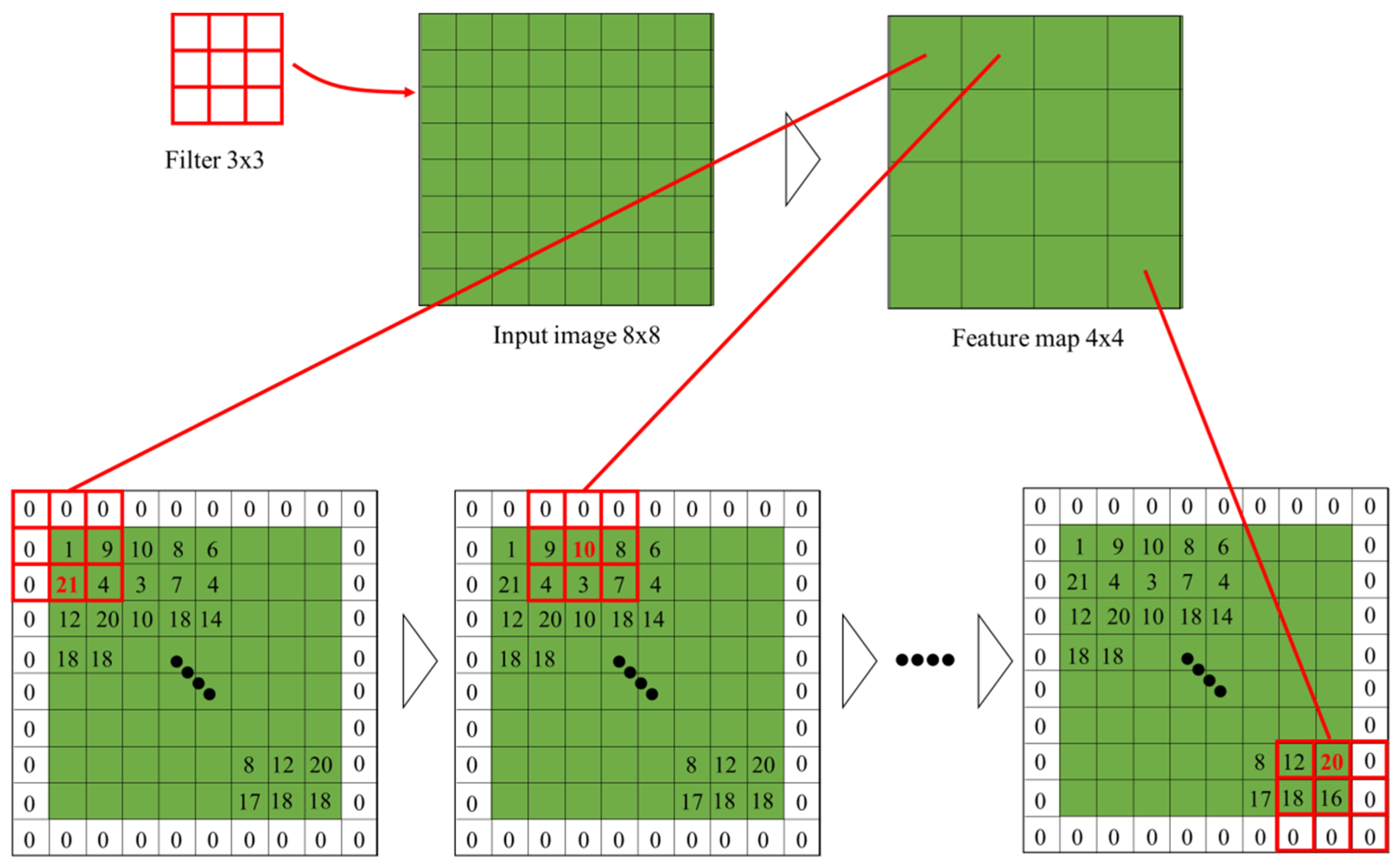For all image sizes, the decrease in A_c for 90° and 270° was about 20% for x_d = 15δ and within 10% for the other x_d, compared with 0° and 180°. This result shows the robustness to geometrical (rotational) changes. In order to visualize how the image pattern was recognized by the CNN, a part of the feature map of the pooling layer per each rotation image is shown in Figure 3d. This feature map was based on the correct answer verification image of x_d = 20δ for W0.225δ. For the first pooling layer (“Pooling 1” in Figure 3d), an image having a window size of 0.225δ was entered as an input with a data size of 224 × 224 × 3 channels, becoming 54 × 54 × 64 channels with a 3 × 3 filter in “Pooling 1.” Some results of four filters at this pooling layer were displayed as images at the same position and labelled as a-1 and a-2 for all rotated images. From these images of “Pooling 1”, it can be seen that the same filter extracted nearly the same features regardless of rotation. The same tendency can be confirmed in the deeper layers; thus, the deeper the layers, the more relaxed the positional relationship of the reaction. At the final softmax, the estimation was successful because all the feature maps show the same distribution for all rotation cases. The red-highlighted panel at b-1 in the softmax image in the figure was the correct answer, and the redder the value, the higher the classification accuracy.

Although the CNN has robustness to the parallel displacement of features owing to the pooling process, it was considered that the robustness to rotation was not so strong in the literature. In this experimental system, the dye released from the diffusion source was diffused downstream while rotating with the vortex motions in the channel turbulence. Hence, when the CNN extracts the characteristics of the patch generated by the small eddies without anisotropy, highly robust estimation against rotation can be possible. Some features not depending on image rotation were included in the dye patch and extracted by the CNN for the x_d prediction with better accuracy.

To evaluate the relation between the turbulent characteristics and the feature map, we focused on the turbulent length scales. Typical scales that characterize turbulence include the integral length scale and the Taylor microscale, which can be calculated from the two-point correlation coefficient. The former is the macro-length scale that the motion of the fluid mass at a certain point can influence, and the latter is the smallest scale caused by the turbulent motion (e.g., vortex). Regarding the images used for learning, each scale was obtained from the concentration distribution statistics of each x_d. The integral characteristic length, L, was calculated by the following equation:

$$L={{\displaystyle \int }}^{ }{R}_{CC}\left(r\right)\mathrm{d}r,$$

(1)

where r is a spatial two-point distance vector. The autocorrelation coefficient, R_cc (r), is calculated by

$$R_{CC}\left(r\right)=\frac{\overline{C{}^{\prime }\left(x\right)C{}^{\prime }\left(x+r\right)}}{\overline{C{}^{\prime }\left(x\right)C{}^{\prime }\left(x\right)}}.$$

(2)

Here, the overbar denotes the ensemble average. The local dye density, C(x), is considered proportional to the brightness fluctuation value of each pixel calculated from the image data. Its fluctuating component, C′(x), is also the brightness value of each pixel minus the average brightness, which was obtained in advance from all image data points. The Taylor microscale, λ_T, was calculated from the following parabolic approximation of the correlation coefficient at r = 0 [31,32]:

$${\lambda }_T={\left[-\frac{1}{2}{\frac{{\mathrm{d}}^2{R}_{CC}\left(r\right)}{\mathrm{d}{r}^2}|}_{r=0}\right]}^{-1/2}.$$

(3)

Figure 4 shows the integral length scale at the channel center and the Taylor microscale, which are calculated by Equations (1)–(3). As the diffusion was emitted from a point source at x_d = 0, the integral length increased as it moved downstream and became nearly constant at x_d = 15δ. This tendency is consistent with another experiment [31], but the value depends on both the Reynolds number and the dye nozzle diameter. In this experiment, the integral length scale was ~0.1δ. Image sizes larger than this (e.g., W0.9δ and W0.225δ) can be expected to extract the characteristics as large as the integral length. However, in W0.05δ, the image size was smaller than the integral length; thus, its characteristics in the large scale could not be captured. Meanwhile, it can be seen that any image size is large enough to extract the features of the Taylor microscale (~0.03δ). Therefore, the estimation was performed using microscale information so that the influence of anisotropy of channel turbulence could be eliminated to some extent. If the source distance could be estimated using only anisotropic features, the estimation would depend on the mainstream conditions, implying macroscale information; thus, the generalization performance would be deteriorated.

As mentioned earlier, from the point source to a medium distance, the concentration mass was distributed not uniformly over the entire channel, resulting in macroscopic concentration non-uniformity. To identify the range of source distance where this non-uniformity affects the accuracy of determination, the distance that the dye flows from the channel center to spread over the entire channel was estimated. The spanwise wavelength of large-scale structures in the channel turbulence is 1.3δ–1.6δ [30], and it is assumed that the dye in the channel center is directed toward the wall vicinity, owing to the vortices related to this large-scale structure and the smaller-scale vortices. Assuming that the advection velocity from the channel center to the wall vicinity is about the same as wall-normal velocity fluctuation, v’, the arrival time from the channel center to the wall surface, t_h, is

$$t_h\approx \delta /v{}^{\prime }$$

(4)

Assuming that the speed at which the dye advances in the streamwise direction is about the same as the bulk velocity, u_b, the distance of x_h traveled in time of t_h is

$$x_h\approx u_b\times t_h=\delta u_b/v{}^{\prime }.$$

(5)

According to DNS database [30], u_b/v’ = 15–20 for Re_τ = 180–640. Then, x_h at Re_b = 18,000 was estimated as follows:

$$x_h\approx 15\delta ~20\delta$$

(6)

Therefore, the distance after which the macroscopic non-uniformity of the dye becomes less significant is estimated to be past x_d = 15δ–20δ. It is assumed that the accuracy of determination of the rotated images at 90° and 270° hardly decreased at x_d ≥ 20δ, because the non-uniformity of the dye was alleviated.

3.3. Effect on Accuracy of Inference by Spot Dye Scale and Arrangement

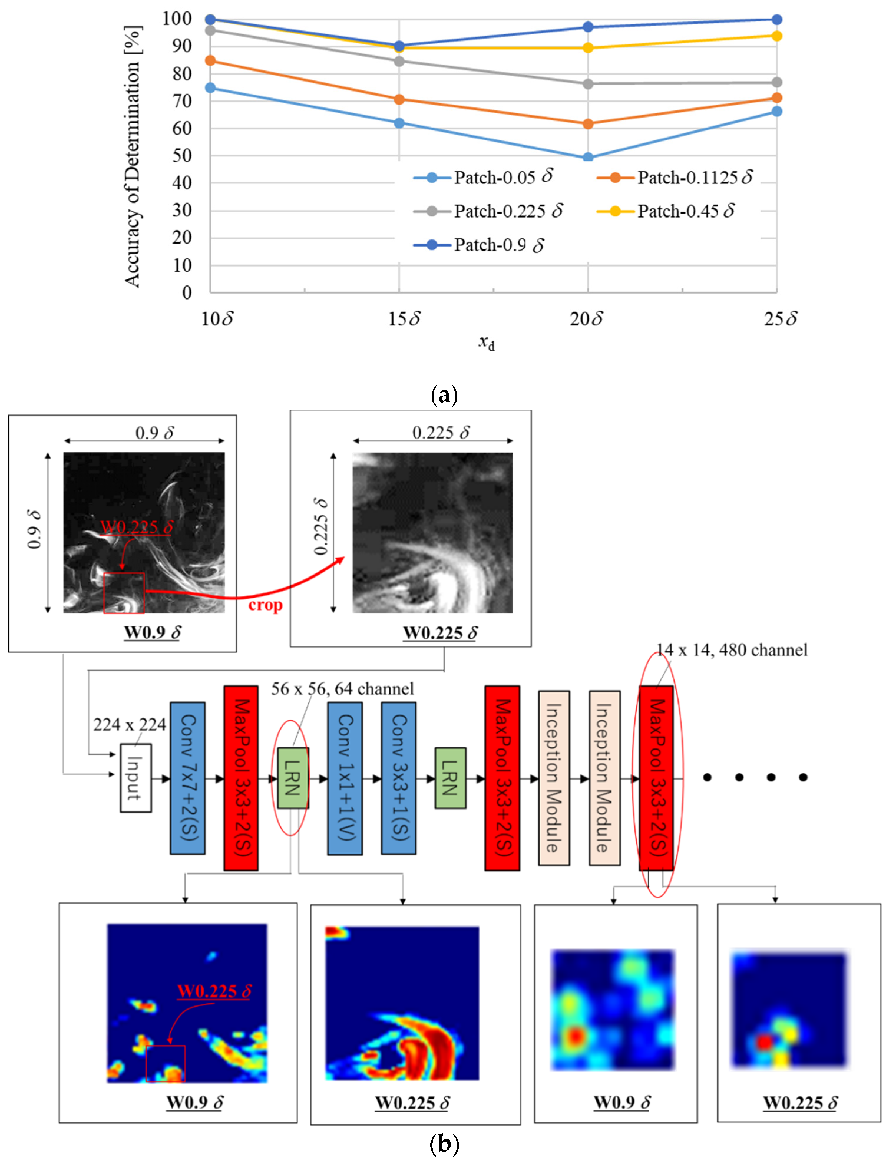
To investigate the effect of the measurement window size on the prediction accuracy, we compared accuracies using images of different window sizes. Classification was conducted for five sizes (W0.9δ, W0.45δ, W0.225δ, W0.1125δ, and W0.05δ) using four classes (x_d = 10δ, 15δ, 20δ, and 25δ). The estimation result is shown in Figure 5a. The large window cases of W0.9δ and W0.45δ provided an accuracy of determination, A_c, of 90% regardless of distance x_d. However, for smaller window sizes, A_c drops sharply at 20δ and 25δ, reaching about 50–80%. Considering that the diameter of the vortex involved in the large-scale structure of channel turbulence was about 0.6δ [30], an image size equivalent to about half of this is necessary for improving the classification accuracy. Additionally, as mentioned earlier, measurement window sizes of <0.225δ are smaller than the integral characteristic length; thus, it is possible that the turbulent flow characteristics of this scale could not also be extracted. The narrowness of the observation window affected the estimation results.

To verify the patch scale extracted from the feature map, we focused on W0.9δ and W0.225δ at the same x_d, which show different values in A_c. For the verification, an image of W0.9δ at x_d = 20δ (with A_c > 95%) and an image obtained by cutting out a part of the W0.9δ image were used for verification of W0.225δ (see Figure 5b, A_c < 78%). This allows us to determine whether features were extracted for the same patch among different patch sizes. Both test images were successfully estimated by each trained CNN. Figure 5b shows the images recognized at each layer of the trained CNN. In the first local response normalization (LRN) in GoogLeNet, one can see that the patch cut out by W0.225δ was extracted in both cases. Meanwhile, in W0.9δ, which had a high percentage of A_c, in addition to the patch cut out by W0.225δ, another patch near it was extracted. In the third pooling layer, a deeper layer, featured on a large scale of about 0.9δ was extracted. This suggests that rather than a single patch, the spatial arrangement pattern of multiple small patches may affect the accuracy. This is consistent with the knowledge of vortex diameters involved in the large-scale structures of channel turbulence.

To confirm the effect of the relatively small patch-placement pattern in a single image on the estimation, we used a test image in which a part of the image was intentionally made defective for W0.9δ; the effect on estimation was confirmed using a trained CNN with four classes having defect-free images. The defective part has a brightness value of zero, i.e., black. The image defect pattern is shown in

Table 2. Accuracy of determination for partially defected images. N_d = 416 for each case.

Case	Original	A	B	C
Partially defected images
Accuracy of Determination
10δ	100.0%	98.1%	96.2%	53.8%
15δ	90.4%	83.7%	78.8%	81.7%
20δ	97.1%	97.1%	93.3%	63.5%
25δ	100.0%	99.0%	8.7%	1.9%

. The same processing was performed on all original test images, i.e., 416 images × 3 patterns (A, B, and C). The size comparison of the defective region was A < B < C. Table 2 shows A_c for each pattern. It is confirmed that the determination accuracy tended to be significantly worse downstream at x_d = 25δ as the area of defects increased. In contrast, at x_d = 15δ, the accuracy of determination was close to 80%, even in a pattern having many defects. This implies that the patch pattern is a more necessary factor for correct estimation as x_d increases.

It is thought that the trained CNN extracted the characteristic scale of channel turbulence from the patch size and pattern within each image. Then, we attempted to confirm the characteristic scale of concentration fluctuation, C’, in each image using two-dimensional power spectrum density (2D PSD) analysis of luminance fluctuation.

Figure 6a shows the 2D PSD results for W0.9δ, which is the largest image size. In addition to the arbitrarily chosen instant images and their analytic results, the ensemble-averaged spectra are also shown. The top images are samples for input data; each lower figure shows the 2D spectrum of each input image, and the right figure is an ensemble-averaged 2D spectrum. All shown input images are typical images that can be estimated for each source distance accurately by the trained CNN in the case of W0.9δ. Figure 6b,c show the one-dimensional PSD on the line (k_x = k_y) tilted 45° from the origin of (k_x, k_y) = (0, 0), marked with a red line in the images of (a) from each input image. However, no clear characteristic peak is found other than that at the origin. When statistically processed, the spectrum becomes gradual, and the scalar fluctuation energy decreases continuously at each scale, and any characteristic wave number cannot be confirmed, such as the spectra of the instant images. Figure 6d,e show the pre-multiplied spectra on the same straight line as the one shown in Figure 6a. As with the PSD, no clear peaks can be seen in the instant images. When the ensemble average was used, the peak wavenumber was confirmed to be within 10δ–25δ. However, this is the peak that appeared using the ensemble average; hence, the clear peak wavenumber could not be detected in the instant images (Figure 6a). We can conclude that, in contrast to the conventional feature extraction (i.e., PSD analysis), which requires time statistics, the CNN has an advantage of estimating the distance from ‘instantaneous’ information.

3.4. Factors for Reducing Prediction Accuracy

In this study, an ideal specific condition (i.e., channel flow, one Reynolds number, and fixed camera angle) was used to produce training data for the CNN. The generalization performance of the learner should be examined in view of practical applications. We evaluated the generalization performance by test images that are intentionally transformed by window size and image quality. This provides a discussion regarding factors that reduce prediction accuracy in actual scenarios.

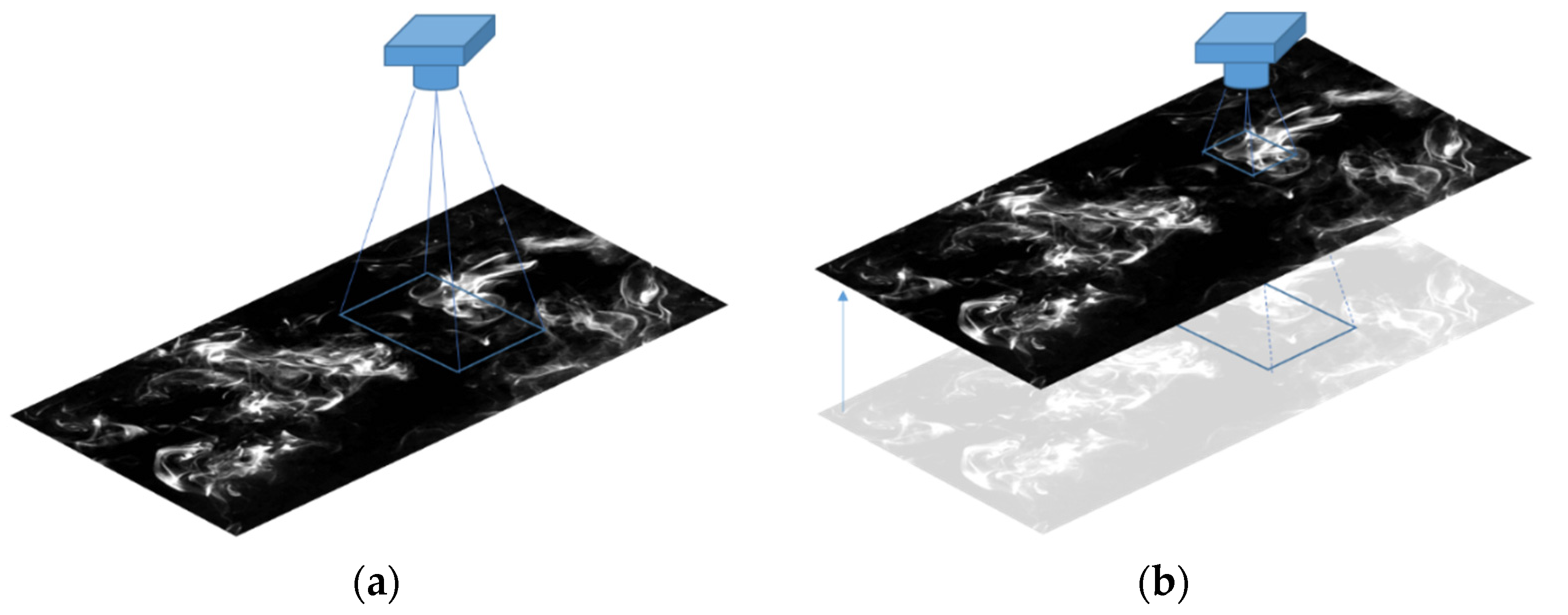
Firstly, we consider the situation that the camera distance from the measurement plane differs between training and testing, as shown in Figure 7. The influence of incorrect window size, i.e., incorrect camera distance, on the prediction accuracy was evaluated for two situations. As one of the situations where the test image whose window size is larger than that of training images, the W0.05δ learner was ‘incorrectly’ applied for the W0.9δ image input. As for the other situation, the W0.9δ learner was chosen to test a smaller window size (W0.05δ) than the image size assumed by the learner. Sample images for W0.05δ and W0.9δ at several x_d are shown in Figure 8. Since the dye was not sufficiently diffused at 10δ, a clear dye pattern can be captured even within the window size of W0.05δ. 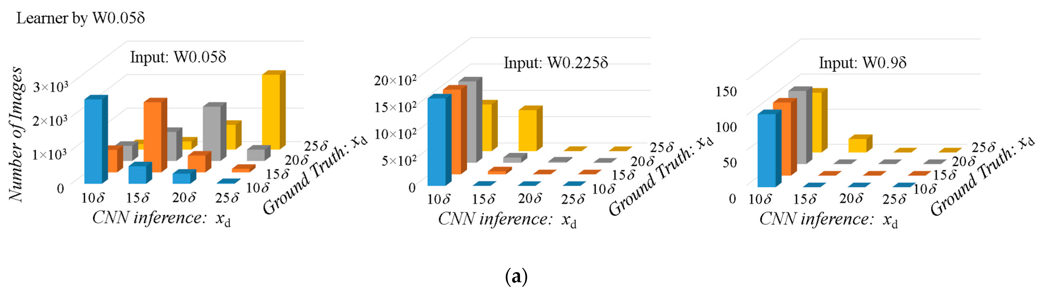On the other hand, the dye is more spread by turbulent mixing at 20δ and 25δ, which causes difficulty in capturing a clear dye pattern within the small window size of W0.05δ. It means that almost uniform dye might cover the whole W0.05δ window size. When an image of W0.9δ is used for test input image of the learner created by W0.05δ, the input image which contains clear dye shading is recognized as “not diffusing well” and the source distance, x_d, is underestimated. In fact, when the test images of W0.9δ are used as the input images for the W0.05δ learner, they are inferred to be 10δ at all positions, as shown in Figure 9a. This must be the same as scaling down in the representative length of turbulence (i.e., image window size in this study) and using a pseudo low-Re image as an input. Similarly, when an image with W0.05δ is input to a learner trained with W0.9δ, it is considered to have a higher Re than the actual image and is resulting in an overestimated x_d, as shown in Figure 9b.

Next, we discuss the effect of the difference in the image quality (in terms of noise and image compression) between the training and testing images. We add Gaussian noise to some images to check the robustness against random noise, as the same approach in the literature [33,34]. This noise addition does not affect the white pixel with the maximum luminance, while the originally black pixel would be affected significantly. The accuracy of determination averaged over the four classes for the learner trained by W0.9δ was plotted with the different noise intensity, as shown in Figure 10. The Gaussian noise input, whose mean value is 0, with a standard deviation of 1.0 for the luminance of image degraded the accuracy by 10%. More specifically, there was a significant decrease in inference accuracy, especially upstream, such as x_d = 10δ and 15δ, with little effect on the downstream side (figure not shown). This may be because a small amount of noise introduced “pseudo dye patches” into the non-distributed area, which is a characteristic of the upstream image. Since the dye diffusion has not yet progressed in the relatively upstream area immediately after the diffusion source, the distribution of the dye is clearly divided into black and white (with less gray regions), and the dye-absent area tends to be completely black with zero luminance. This feature was impaired by noise, which led to a decrease in the inference accuracy on the upstream side. The Gaussian noise with a standard deviation of 0.1 might be acceptable for this feature. On the other hand, when stronger noise with a standard deviation of 5.0 was added, the inference accuracy on the downstream side as well as the upstream side dropped significantly. As a result, the overall inference accuracy decreased down to 41%. On the downstream side, which was more robust to a weak noise, the image was generally more luminous, but the dye patches exhibited a fine filament-like pattern. This feature was lost by the strong noise and caused the inference accuracy to decline. Both inaccuracies were due to the loss of features in the distribution of the dye patches. Results with a standard deviation of 100 are interesting as well. Note that the inferential accuracy value is 25%, but it was validated on a four-class classification problem. This means that the inference of the learner did not work at all. For all noise-added images, the learner trained on noiseless images produced an output of x_d = 10δ. In fact, the input image with a standard deviation of 100 would rather appear to anyone as a white image (see the rightest image in Figure 10). Such an extensive whitening feature seen in this image is observed upstream near the diffuse source. Therefore, the prediction mistake is a rather reasonable result for the trained learner.

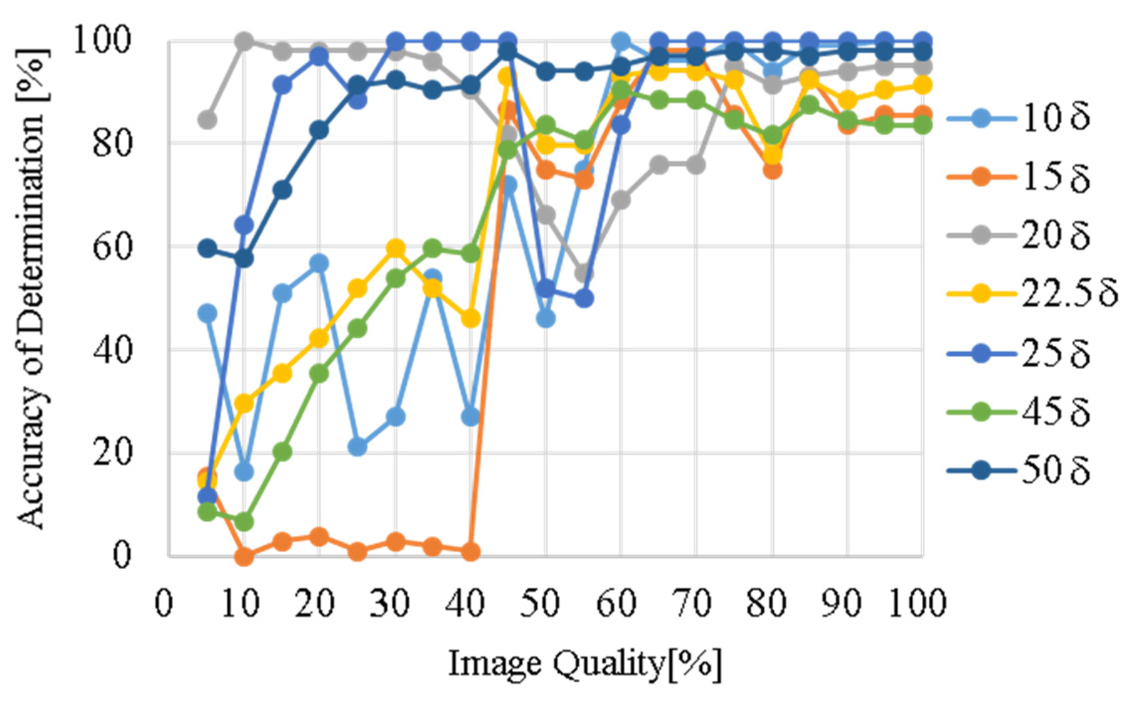
We also confirmed the effect of image quality on the prediction accuracy by the image compression of JPEG format by the learner of W0.9δ over seven classes. Figure 11 shows the dependency on the image quality for seven classes of W0.9δ, where the low/high image quality means the small/large file size with high/low compression rate. We found that the image quality of >85% provides the almost same A_c irrespectively of x_d. However, for the image quality of <40%, the accuracy is deteriorated significantly at several locations of 10δ, 15δ, 22.5δ, and 45δ. This deterioration must be because the delicate filament structure of dye patches created by turbulent motions is blurred in the image compression. In other words, the low image quality that does not capture the dye filament is fatal in the estimation based on the dye pattern under turbulent diffusion.

As discussed above, the present trained CNN still have a weakness against ambiguous window size and strong noise (or image compression) to blur the delicate filament structure of dye patches. As discussed above, the key to the inference accuracy in the present method is to extract the “turbulent diffusion” of passive-scalar dye. The inhomogeneous dye distribution and the dye patches stretched into filaments due to successive turbulent motions have important information related to the diffuse source distance. Given a low Schmidt number, such informative dye patches would be immediately dissipated by molecular diffusion, resulting in malfunction of the learner. On the other hand, a high Schmidt number is rather favorable, and the learner is expected to work as long as very fine filamentary dye patches can be resolved. Compared to the Schmidt number, the dependence on the Reynolds number might be moderate. However, due to highly turbulent mixing under significantly high Reynolds number, the inference accuracy would be decreased since the dye distribution would be lost quickly even at moderate Schmidt number. As the same reason, if there is no change of dye distributions in each x_d under a low Reynolds number close to the laminar regime, the inference accuracy might be low.

4. Conclusions

We investigated the applicability of CNN image recognition technology to turbulent material diffusion point-source prediction with the aim of establishing a pollutant-leak source prediction technology using 2D image information. The target system was a 2D channel turbulent flow, and the point-source distance was estimated with a CNN using dye images taken downstream. The diffusion source distance, x_d, of each image was estimated as a classification problem using instantaneous PLIF density images at seven locations in the range of x_d = 10δ–50δ, downstream from the point source (x_d = 0) as training and testing data.

To investigate the effect of different CNN architectures on the prediction performance, we verified the prediction accuracy of several network models. Deep-layer models other than LeNet, which included AlexNet, GoogLeNet, and Inception-ResNet-v2, had an accuracy of >75%. Thus, we confirmed the success of the source-distance estimation of the deep CNN. In particular, GoogLeNet and Inception-ResNet-v2 had an accuracy better than 90%, and it was confirmed that the deeper the network, the higher the accuracy. In terms of computational cost, GoogLeNet with 22 layers may have been optimal, whereas Inception-ResNet-v2 with 164 layers spent 4–6 times longer and showed only a few-percent performance improvement. Both LeNet and AlexNet were not demanding, but there were significant decreases in inference accuracy with respect to the number of layers. There is probably an optimal number of layers that is cost-effective, and in the present subject, that was about 20 layers.

The geometrical change (rotation) of the test image caused a decrease in the prediction accuracy of ~10–20% at x_d = 15δ, but the robustness of the estimation, regardless of the anisotropy of the concentration distribution, was demonstrated. The image size and resolution sufficiently captured the Taylor microscale, and good estimation was made based on microscale information that eliminated the influence of channel turbulence anisotropy to some extent. The decrease in robustness with respect to rotation at x_d = 15δ was caused by the non-uniformity of the dye flowing from a point source that is very small, relatively, to the channel width.

To focus on the effect of large-scale turbulent characteristics on the prediction accuracy, we compared accuracies using images of different window sizes. The prediction was improved when a window size was larger than the integral characteristic length and comparable to the large-scale structure of channel turbulence. In images having these window sizes, the positional relationships of the patches on a relatively small scale were extracted as a feature, and it was confirmed that the prediction accuracy improved.

We attempted to extract the characteristic scale of each image using the conventional linear analysis PSD method, showing that the characteristics could be confirmed to some extent by statistical processing. However, using CNN, it was possible to estimate the diffusion source distance with an accuracy higher than that of PSD using instantaneous data without statistical processing. Therefore, the spatial distribution information of patches appearing in statistical processing can be used for CNN estimation.

We demonstrated the feasibility of CNN to estimate the turbulent diffusion source for a simple flow of the wall turbulence. This study was limited to a single set of a Reynolds number and Schmidt number, and the verification was limited to a point-source distance up to x_d = 50δ of a unidirectional, steady turbulent flow. In order to understand the generalization performance of the learner, test images which are intentionally transformed by aspects such as window size and image quality were examined by the learner. This will provide the camera distance from the measurement plane for training and testing. As discussed above, the present trained CNN still has its weakness against ambiguous window size and strong noise (or image compression to blur the delicate filament structure of dye patches). To use the simulation data for training images instead of actual leaked images, we need to carefully handle the test images for obtaining the high prediction accuracy. In the future, in addition to the conditions of high Re, it will be necessary to anticipate actual uses and to investigate the effects of main-flow changes on estimation accuracy, including spatial changes in obstacles and curved pipes, and temporal changes caused by non-stationarity.

References

1. Liu, X.; Zhai, Z. Inverse modeling methods for indoor airborne pollutant tracking: Literature review and fundamentals. Indoor Air 2007, 17, 419–438. [Google Scholar] [CrossRef] [PubMed]
2. Tsukahara, T.; Oyagi, K.; Kawaguchi, Y. Estimation method to identify scalar point source in turbulent flow based on Taylor’s diffusion theory. Environ. Fluid Mech. 2016, 16, 521–537. [Google Scholar] [CrossRef]
3. Ababou, R.; Bagtzoglou, A.C.; Mallet, A. Anti-diffusion and source identification with the ‘RAW’ scheme: A particle-based censored random walk. Environ. Fluid Mech. 2010, 10, 41–76. [Google Scholar] [CrossRef]
4. Abe, S.; Kato, S.; Hamba, F.; Kitazawa, D. Study on the dependence of reverse simulation for identifying a pollutant source on grid resolution and filter width in cavity flow. J. Appl. Math. 2012, 2012, 847864. [Google Scholar] [CrossRef]
5. Cerizza, D.; Sekiguchi, W.; Tsukahara, T.; Zaki, T.A.; Hasegawa, Y. Reconstruction of scalar source intensity based on sensor signal in turbulent channel flow. Flow Turbul. Combust. 2016, 97, 1211–1233. [Google Scholar] [CrossRef]
6. Rajaona, H.; Septier, F.; Armand, P.; Delignon, Y.; Olry, C.; Albergel, A.; Moussafir, J. An adaptive Bayesian inference algorithm to estimate the parameters of a hazardous atmospheric release. Atmos. Environ. 2015, 122, 748–762. [Google Scholar] [CrossRef]
7. Shao, Q.; Sekine, D.; Tsukahara, T.; Kawaguchi, Y. Inverse source locating method based on graphical analysis of dye plume images in a turbulent flow. Open J. Fluid Dyn. 2016, 6, 343–360. [Google Scholar] [CrossRef] [Green Version]
8. Geer, A.J. Learning earth system models from observations: Machine learning or data assimilation? Philos. Trans. R. Soc. A 2021, 379, 20200089. [Google Scholar] [CrossRef]
9. Tsuduki, S. Advanced wide area gas monitoring system. In Proceedings of the Japan Petrol Inst 50th Petrol Petrochem Forum, Kumamoto, Japan, 12–13 November 2020. (In Japanese). [Google Scholar]
10. LeCun, Y.; Bottou, L.; Bengio, Y.; Haffner, P. Gradient-based learning applied document recognition. Proc. IEEE 1998, 88, 2278–2324. [Google Scholar] [CrossRef] [Green Version]
11. Krizhevsky, A.; Sutskever, I.; Hinton, G.E. ImageNet classification with deep convolutional neural networks. Adv. Neural Inf. Process. Syst. 2012, 25, 1097–1105. [Google Scholar] [CrossRef]
12. Szegedy, C.; Liu, W.; Jia, Y.; Sermanet, P.; Reed, S.; Anguelov, D.; Erhan, D.; Vanhoucke, V.; Rabinovich, A. Going deeper with convolutions. In Proceedings of the IEEE Conference on Computer Vision and Pattern Recognition, Boston, MA, USA, 7–12 June 2015; pp. 1–9. [Google Scholar]
13. He, K.; Zhang, X.; Ren, S.; Sun, J. Deep residual learning for image recognition. In Proceedings of the IEEE Conference on Computer Vision and Pattern Recognition, Las Vegas, NV, USA, 27–30 June 2016; pp. 770–778. [Google Scholar]
14. Huang, G.; Liu, Z.; Van der Maaten, L.; Weinberger, K.Q. Densely connected convolutional networks. In Proceedings of the IEEE Conference on Computer Vision and Pattern Recognition, Honolulu, HI, USA, 21–26 July 2017; pp. 4700–4708. [Google Scholar]
15. Szegedy, C.; Ioffe, S.; Vanhoucke, V.; Alemi, A. Inception-v4, Inception-ResNet and the impact of residual connections on learning. In Proceedings of the Thirty-First AAAI Conference on Artificial Intelligence, San Francisco, CA, USA, 4–9 February 2017; pp. 4278–4284. [Google Scholar]
16. Bressem, K.K.; Adams, L.C.; Erxleben, C.; Hamm, B.; Niehues, S.M.; Vahldiek, J.L. Comparing different deep learning architectures for classification of chest radiographs. Sci. Rep. 2020, 10, 13590. [Google Scholar] [CrossRef]
17. Pham, T.D. A comprehensive study on classification of COVID-19 on computed tomography with pretrained convolutional neural networks. Sci. Rep. 2020, 10, 16942. [Google Scholar] [CrossRef] [PubMed]
18. Diana, L.; Xu, J.; Fanucci, L. Oil spill identification from SAR images for low power embedded systems using CNN. Remote Sens. 2021, 13, 3606. [Google Scholar] [CrossRef]
19. Seydi, S.T.; Hasanlou, M.; Amani, M.; Huang, W. Oil spill detection based on multiscale multidimensional residual CNN for optical remote sensing imagery. IEEE J. Sel. Top. Appl. Earth Obs. Remote Sens. 2021, 14, 10941–10952. [Google Scholar] [CrossRef]
20. Qin, D.; Yu, J.; Zou, G.; Yong, R.; Zhao, Q.; Zhang, B. A novel combined prediction scheme based on CNN and LSTM for urban PM2.5 concentration. IEEE Access 2019, 7, 20050–20059. [Google Scholar] [CrossRef]
21. Duraisamy, K.; Iaccarino, G.; Xiao, H. Turbulence modeling in the age of data. Annu. Rev. Fluid Mech. 2019, 51, 357–377. [Google Scholar] [CrossRef] [Green Version]
22. Brunton, S.L.; Noack, B.R.; Koumoutsakos, P. Machine learning for fluid mechanics. Annu. Rev. Fluid Mech. 2020, 52, 477–508. [Google Scholar] [CrossRef] [Green Version]
23. Fukami, K.; Fukagata, K.; Taira, K. Assessment of supervised machine learning methods for fluid flows. Theor. Comput. Fluid Dyn. 2020, 34, 497–519. [Google Scholar] [CrossRef] [Green Version]
24. Brenner, M.P.; Eldredge, J.D.; Freund, J.B. Perspective on machine learning for advancing fluid mechanics. Phys. Rev. Fluids 2019, 4, 100501. [Google Scholar] [CrossRef]
25. Fukami, K.; Nabae, Y.; Kawai, K.; Fukagata, K. Synthetic turbulent inflow generator using machine learning. Phys. Rev. Fluids 2019, 4, 064603. [Google Scholar] [CrossRef] [Green Version]
26. Fukami, K.; Nakamura, T.; Fukagata, K. Convolutional neural network based hierarchical autoencoder for nonlinear mode decomposition of fluid field data. Phys. Fluids 2020, 32, 095110. [Google Scholar] [CrossRef]
27. Fukami, K.; Fukagata, K.; Taira, K. Super-resolution reconstruction of turbulent flows with machine learning. J. Fluid Mech. 2019, 870, 106–120. [Google Scholar] [CrossRef] [Green Version]
28. Beck, A.; Kurz, M. A perspective on machine learning methods in turbulence modeling. GAMM-Mitteilungen 2021, 44, e202100002. [Google Scholar] [CrossRef]
29. Davidson, P.A. Turbulence: An Introduction for Scientists and Engineers; Oxford University Press: Oxford, UK, 2015. [Google Scholar]
30. Abe, H.; Kawamura, H.; Choi, H. Very large-scale structures and their effects on the wall shear-stress fluctuations in a turbulent channel flow up to Reτ = 640. J. Fluids Eng. 2004, 126, 835–843. [Google Scholar] [CrossRef]
31. Mohaghar, M.; Carter, J.; Musci, B.; Reilly, D.; McFarland, J.; Ranjan, D. Evaluation of turbulent mixing transition in a shock-driven variable-density flow. J. Fluid Mech. 2017, 831, 779–825. [Google Scholar] [CrossRef]
32. Mohaghar, M.; Dasi, L.P.; Webster, D.R. Scalar power spectra and turbulent scalar length scales of high-Schmidt-number passive scalar fields in turbulent boundary layers. Phys. Rev. Fluids 2020, 5, 084606. [Google Scholar] [CrossRef]
33. Morimoto, M.; Fukami, K.; Fukagata, K. Experimental velocity data estimation for imperfect particle images using machine learning. Phys. Fluids 2021, 33, 087121. [Google Scholar] [CrossRef]
34. Buzzicotti, M.; Bonaccorso, F.; Di Leoni, P.C.; Biferale, L. Reconstruction of turbulent data with deep generative models for semantic inpainting from TURB-Rot database. Phys. Rev. Fluids 2021, 6, 050503. [Google Scholar] [CrossRef]
Figure 1. (a) Schematic of experimental setup; YAG = yttrium aluminum garnet. (b) Samples of original images (1.8δ × 3.6δ) including multi−scale patches in a dye pattern. Flow direction is from left to right.
Processes 10 00860 g001aProcesses 10 00860 g001b
Figure 2. Accuracy of determination of W0.9δ by each network model including different network depths. The average accuracy over seven classes (i.e., seven different xd) are also shown.
Processes 10 00860 g002
Figure 3. Accuracy of determination for rotated images: (a) W0.9δ, (b) W0.225δ, and (c) W0.05δ. This CNN was trained by original image (0°). (d) Feature map for each pooling layer for each rotated image based on the correct answer verification image of x d = 20δ for W0.225δ.
Processes 10 00860 g003aProcesses 10 00860 g003b
Figure 4. Length scale related to fluctuated scalar concentration field as a function of the distance from the scalar source: (a) integral length scale, L, and (b) scalar Taylor microscale, λT.
Processes 10 00860 g004aProcesses 10 00860 g004b
Figure 5. (a) Accuracy of determination for each patch size. (b) Sample images for a feature map of first LRN and third max pool in W0.9δ and W0.225δ.
Processes 10 00860 g005
Figure 6. Two-dimensional power spectrum density (2D PSD) of concentration fluctuation fields. (a) Analysis procedure and averaged spectral density distribution. (b) PSDs on 45° line indicated as a red line in the images of (a). (c) Same as (b) but for the ensemble-averaged PSDs. (d) Same as (b) but for the pre-multiplied spectrum of PSD for scalar fluctuation. (e) Same as (b) but for pre-multiplied spectrum of PSD.
Processes 10 00860 g006aProcesses 10 00860 g006b
Figure 7. Camera distance from the measurement plane: (a) the original distance of image acquisition for training of the learner; (b) the incorrect camera distance, which results in a wrongly zoomed-up image to be input by the learner.
Processes 10 00860 g007
Figure 8. Sample images of W0.9δ and zoomed-up W0.05δ with the same image size.
Processes 10 00860 g008
Figure 9. Prediction accuracy with mismatch in the window size between the learner and test input images. (a) Learner of W0.05δ; (b) learner of W0.9δ, which, of course, provides a good performance when the window sizes are matched between the training image (the learner) and testing image.
Processes 10 00860 g009aProcesses 10 00860 g009b
Figure 10. Accuracy of determination with noisy input image for four classes of W0.9δ by Gaussian noise with a zero mean for the luminance of image.
Processes 10 00860 g010
Figure 11. Dependence of the prediction accuracy on the image quality for seven classes of W0.9δ.
Processes 10 00860 g011