A Machine Learning Approach for Phase-Split Calculations in n-Octane/Water and PASN/Water Systems

Abstract

Flash calculations, including phase split and phase classification for both n-octane/water blends and paraffinic aromatic synthetic naphtha (PASN)/water blends present significant computational challenges. Calculations to establish the two-phase and three-phase regions, as well as the transitions between regions, were addressed by a phase classification method proposed in a recent contribution involving machine learning (ML). This work focusses on the phase-split calculations, considering (a) the lack of numerical convergence of the traditional calculations and their related numerical issues for water/n-octane and PASN/water systems based on the Rachford–Rice derived surfaces and (b) the successful implementation of an ML approach based on a K-nearest-neighbor (KNN) algorithm, which uses the abundant experimental data obtained in a CREC-VL cell.

1. Introduction

Phase equilibrium calculations deal with two main problems [1]: (i) phase stability or the number of phases present, and (ii) phase split or the establishment of the composition and amount of each phase present. For water/hydrocarbon mixtures, conventional approaches to determine phase equilibrium are computationally expensive. Furthermore, the various analyses are penalized by the lack of good initial estimates of equilibrium phase ratios [2,3].

While the number of phases at thermodynamic equilibrium is an unknown condition, as considered in our previous work [4,5,6], experimental data from the CREC-VL cell can be used to determine whether two-phase or three-phase regions are present. This allows for, in combination with ML, an effective “a priori” classification of the number of phases. This also reduces the computational cost and gives better initial estimates of the phase-split calculation once the model is trained.

Traditionally, the designated Rachford–Rice equations [7] can be used to solve the phase-split calculations for a flash unit (Figure 1 and Figure 2). The equations for both two-phase and three-phase calculations are summarized in Equations (1)–(3).

$$F\left(\beta \right)={\displaystyle \sum }_{i=1}^N\frac{z_i\left(K_i-1\right)}{1+\beta \left(K_i-1\right)}=0$$

(1)

$$F\left(\beta \right)={\displaystyle \sum }_{i=1}^N\frac{z_i\left(K_i^m-1\right)}{H_i}=0$$

(2)

$$H_i=1+{\beta }^L\left(K_i^L-1\right)+{\beta }^W\left(K_i^W-1\right)$$

(3)

where $\beta$ corresponds to the vapor mole fraction, z_i is the molar fraction of component i, K_i stand for the equilibrium constants, and H_i is an auxiliary variable.

Calculations using the Rachford–Rice equations may involve different numerical approaches as reported in the technical literature, such as successive substitution, quasi-Newton, Newton, steepest-descend, and their modifications and combinations [2].

In the present study, two-phase and three -flash calculations are specifically developed for water/n-octane and PASN/water blends using the Soave–Redlich–Kwong–Kabadi–Danner equation of state (SRKKD EoS). Following this, convergence calculations and numerical issues for water/n-octane and for PASN/water systems are established by using the resulting Rachford–Rice derived surfaces. Once this is accomplished, phase-split computations are compared with those from the ML approach in terms of vapor pressure. The outcome of this highlights the importance of an ML approach for accurate predictions, which is developed quite effectively by using the abundant research data available from the CREC-VL Cell experiments [8].

2. Mathematical Model

Soave–Redlich–Kwong–Kabadi–Danner (SRKKD) Equation of State

Traditionally, the Peng–Robinson (PR) equation of state (EoS) is one of the most popular EoSs, for calculating hydrocarbon-based PVT behavior, including vapor pressures [9]. When using simulation software, such as HYSYS V9 or Aspen Plus V9, it is considered one of the most improved thermodynamic models available, given its large binary interaction parameter database.

However, the PR EoS displays limitations when it is considered for water or aqueous hydrocarbon mixtures [10]. In these cases, as suggested by previous research from our CREC-UWO group [8], the PR EoS does not describe well the system under study, and a different EoS must be used. In binary systems, such as n-octane/water mixtures, an activity coefficient model can be used, as we proposed in our previous work [4].

Nevertheless, classical activity coefficient models are limited to low pressures (≤10 bar) with no C₇₊ species included. In the case of water and heavy hydrocarbons, such as naphtha or bitumen (C₇₊), as in the present study, a cubic equation of state is strongly suggested. In this work, the Soave–Redlich–Kwong (SRK) EoS with a Kabadi–Danner [11] modification is used. These authors suggested that the SRK EoS with Kabadi–Danner modification improves the VLLE calculations for water–hydrocarbon systems, particularly under highly diluted hydrocarbons in water, which is of great interest for this research.

Given the reported advantages of using the Kabadi–Danner modification with the Soave–Redlich–Kwong EoS (SRKKD EoS) for VLL equilibrium calculations for hydrocarbon–water blends [12,13], the SRKKD EoS was used in the present study. The SRKKD EoS can be defined by Equations (4)–(8) as follows:

$$P=\frac{RT}{V-b}-\frac{a}{V\left(V+b\right)}$$

(4)

$$a=0.42748\frac{R^2{T}_C^2}{P_C}{\left[1+\mathsf{\Omega }\left(1-T_r^{1/2}\right)\right]}^2$$

(5)

$$b=0.08664\frac{R{T}_C}{P_C}$$

(6)

$$\mathsf{\Omega }=0.480+1.574\mathsf{\omega }-0.176{\mathsf{\omega }}^2$$

(7)

$$Z^3-Z^2+\left(A^{\prime }-B^{\prime }-{B^{\prime }}^2\right)Z-A^{\prime }{B}^{\prime }=0$$

(8)

where $A^{\prime }=\frac{aP}{{\left(RT\right)}^2}$ and $B^{\prime }=\frac{bP}{RT}$.

The mixing rules required to determine the SRK EoS parameters are given by Equations (10) and (11), with the Kabadi–Danner modification being reported by Equations (9) and (12)–(14) [11].

$$a_{mix}=a_0+a_{KD}$$

(9)

$$a_0={\displaystyle \sum }_{i=1}^N{\displaystyle \sum }_{j=1}^N{x}_i{x}_j\left(1-k_{ij}\right)\sqrt{a_i{a}_j}$$

(10)

$$b_{mix}={\displaystyle \sum }_{i=1}^N{x}_i{b}_i$$

(11)

$$a_{KD}={\displaystyle \sum }_{i=1}^N{a}_{wi}^{″}{x}_w^2{x}_i$$

(12)

$$a_{wi}^{″}=G_i\left[1-{\left(\frac{T}{T_{cw}}\right)}^{0.8}\right]$$

(13)

$$G_i={\displaystyle \sum }_l{g}_l$$

(14)

With respect to $G_i$, it can be calculated using group contribution methods, which account for the sum of the contributions of the different functional groups included in every hydrocarbon molecule. Values from various functional groups can be obtained from the table published by Kabadi–Danner (1985) [11]. The k_ij parameters used for the calculations reported in this work were taken from HYSYS V9 software.

Furthermore, to compute the fugacity coefficient with the SRKKD EoS, Equations (15) and (16) can be used [14] as follows:

$$\ln {\varphi }_i=\frac{b_i}{b}\left(Z-1\right)-\ln \left(Z-B^{\prime }\right)-C_i\prime \ln \frac{Z+B\prime }{Z}$$

(15)

$$C_i^{\prime }=\frac{A\prime }{B\prime }\left(-\frac{b_i}{b}+\frac{2}{a}{\displaystyle \sum }_{j=1}^N{x}_j\sqrt{a_i{a}_j}\left(1-k_{ij}\right)\right)$$

(16)

3. Materials and Methods

3.1. Materials

Distilled water was used with a pH of 7 ± 0.05 and a total organic carbon of less than 0.1 ± 0.02 ppm for all experimental studies. In the case for the alkane compounds, Sigma-Aldrich HPLC assay purity reagents were used. The purity of those hydrocarbons was represented in mole percent as follows: n-hexane >97%, n-heptane >96%, n-octane >99%, n-decane >99%, n-dodecane >99%. The water content of the n-alkanes was 0% for n-octane and n-dodecane, 0.01% for n-hexane and n-decane, and 0.02% for n-heptane. Toluene was obtained from Fisher Scientific with a purity >99% and 0.008% water content.

3.2. CREC Vapor–Liquid Equilibrium Cell

The Chemical Reactor Engineering Center (CREC) developed a CREC VL-Cell [15] that allows for the measurement of VLL equilibrium (Figure 3). This unit uses a “dynamic method”. The temperature of the cell increases progressively by using a thermal ramp of 1.2 °C/min. As a result, every run provides plenty of vapor–liquid equilibrium data at 10 Hz every 0.01 s. Additional explanations about the cell operation are reported in [8,15].

The CREC VL-Cell uses a marine type of impeller (propeller). The unit propeller helps to ensure a well dispersed and homogeneous blend of non-miscible liquids. This provides a good heat distribution inside the CREC VL-Cell. Furthermore, the special cell design allows one to directly analyze a process sample. It also avoids losses of light volatile components due to sample transfers.

The CREC VL-Cell has two thermocouples strategically located inside the CREC VL-Cell and connected to a temperature data acquisition unit. The thermocouples help to measure both the gas- and liquid-phase temperatures within the VL-Cell through a USB desktop computer port. As a result, experimental data can be stored and displayed in real time on a PC using Omega temperature data acquisition software.

In addition to these features, the CREC VL-Cell includes a pressure transducer placed alongside a pressure gauge. The combinations of two separate pressure instruments allows for simultaneous measurement and validation of the saturation vapor pressure. The pressure transducer is logged into a desktop USB port, allowing for observation and registration of the changes of pressure through the Omega software. Thus, one should note that the instrumentation implemented into the CREC VL-Cell delivers accurate temperature and pressure data [15]. In addition, the automatization of the CREC VL-Cell permits the collection of large amounts of vapor pressure data per experiment, which constitute a very valuable source of information for VLL equilibrium simulations and modeling.

4. Results and Discussion

4.1. Traditional Phase-Split Calculations

Traditionally, phase-split calculations are performed by solving Rachford–Rice (RR) equations involving phase equilibrium constants. Rachford–Rice equations are nonlinear functions obtained from the equal chemical potentials combined with species material balances [2].

In the case of the three-phase flash, the main equations (Equations (17)–(21)) are reported below, with the hydrocarbon phase used as a as reference [2,16].

$$f_V\left(\beta \right)=R{R}_V={\displaystyle \sum }_{i=1}^N\left(y_i-x_i^L\right)={\displaystyle \sum }_{i=1}^N\frac{z_i\left(K_i^V-1\right)}{H_i}=0$$

(17)

$$f_W\left(\beta \right)=R{R}_W={\displaystyle \sum }_{i=1}^N\left(x_i^W-x_i^L\right)={\displaystyle \sum }_{i=1}^N\frac{z_i\left(K_i^W-1\right)}{H_i}=0$$

(18)

$$H_i=1+{\beta }^V\left(K_i^V-1\right)+{\beta }^W\left(K_i^W-1\right)$$

(19)

Or

$$f_V\left(\beta \right)={\displaystyle \sum }_{i=1}^N\frac{z_i\left(1-K_i^V\right)}{t_i}=0$$

(20)

$$f_W\left(\beta \right)={\displaystyle \sum }_{i=1}^N\frac{z_i\left(1-K_i^W\right)}{t_i}=0$$

(21)

$$t_i=1-{\beta }^V\left(1-K_i^V\right)-{\beta }^W\left(1-K_i^W\right)$$

(22)

In this respect, the root-finding calculation is a complex one, given these equations present discontinuities at their extremes (division by zero) and may have an almost flat slope near their roots [17].

Additionally, in solving the Rachford–Rice equations, the choice of numerical method is influenced by the independent variables that are selected, such as component mole fractions, equilibrium ratios, or the logarithm of equilibrium ratios [18].

When equilibrium constant ratios or logarithms of equilibrium constants are considered, a Newton–Raphson method is typically applied. In the case of mole fractions, either a Newton method or a minimization of Gibbs free energy can be considered [19]. Logarithms of K calculations are usually preferred, given the use of mole fractions may create an ill-defined Jacobian, and the natural logarithm stabilizes the Newton method when K values of different orders of magnitude are involved [18].

Regarding multiphase flash-split calculations with three or more phases, they typically involve an outer loop, where the equilibrium constants are calculated, and an inner loop, where the mass balances (Rachford–Rice equations) are evaluated. The end goal is to determine the phase mole fractions and the compositions for a given set of K values [20]. This inner loop is known as “constant-K” flash [21].

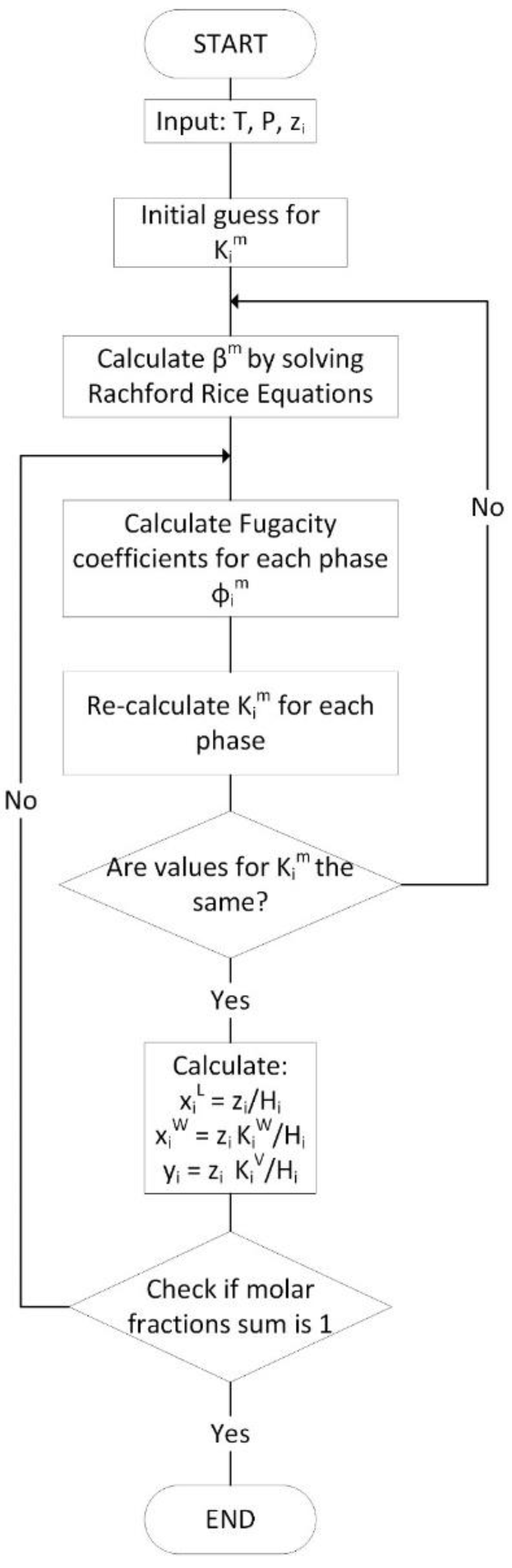
Given the above, a general algorithm to solve multiphase flash calculations is described in Figure 4. It can be observed that within each successive substitution step, the Rachford–Rice equations designated as “constant-K” flash are solved independently.

One should note that the solution of the two-phase constant-K flash calculation is a relatively easy one. However, and in the case where one has to account for a three-phase flash, these calculations may become extensive and challenging. This is due to the non-linearity of the objective resulting functions [18].

The “constant-K” flash is discussed in Section 4.2. In this respect, in phase-split calculations, good initial estimates increase the probability of finding the global minimum Gibbs free energy, with an initial guess from stability testing or the previous simulation timestep being an option [2]. To accomplish this, constraints for the initial estimates are usually needed, as suggested previously by Okuno et al. [20] and Leibovici and Neoschil [22].

4.2. Constant-K Flash Solution

The solution of the “constant-K flash” has been studied previously using two different approaches [24], which include (i) minimization techniques and (ii) direct solution of the RR equations. Tranenstein (1985) [19] proposed a constrained minimization of the Gibbs free energy to solve the two-phase problem, whereas Leibovicy and Jean (1995) [22] used a Newton procedure with a relaxation parameter to solve the multiphase problem. Furthermore, Okuno et al. (2010) [20] minimized the non-monotonic convex function using the independent-phase mole fractions. Haugen et al. (2011) [24] used a two-dimensional bisection method to provide good initial guesses for the Newton algorithm in the three-phase case. Li and Firoozabadi (2012) [2] employed stability testing as an initial guess for phase-split calculations with a two-dimensional bisection method for two and three phases. Yan and Stenby (2014) [25] proposed Householder’s high-order iteration method together with a method to improve the initial estimate for the two-phase problem. More recently, Fernandez-Martinez et al. (2020) [17] applied an associated polynomial to obtain all the roots of a two-phase isothermal flash.

One of the most popular approaches to solve the “constant-K” flash problem is to use a Newton–Raphson method to solve Rachford–Rice equations (Equations (17) and (18)), obtaining values for ${\beta }^V$ and ${\beta }^W$. In that case, the Newton–Raphson method considered is given by Equations (23)–(27).

$${\beta }^{m, new}={\beta }^{m, old}-{\left[\nabla f{\left({\beta }^m\right)}^T\right]}^{-1}\left[f\left({\beta }^m\right)\right]$$

(23)

$${\beta }^{m, new}={\beta }^{m, old}-{\left[J\left({\beta }^m\right)\right]}^{-1}\left[f\left({\beta }^m\right)\right]$$

(24)

$${\beta }^m=\left[\begin{array}{c}{\beta }^V\\ {\beta }^W\end{array}\right]$$

(25)

$$f\left({\beta }^m\right)=\left[\begin{array}{c}{f}_V\left({\beta }^m\right)\\ f_W\left({\beta }^m\right)\end{array}\right]$$

(26)

$$J\left({\beta }^m\right)=\left[\begin{array}{cc}{\displaystyle \sum _{i=1}^N}\frac{-z_i{\left(K_i^V-1\right)}^2}{H_i{}^2}& {\displaystyle \sum _{i=1}^N}\frac{-z_i\left(K_i^V-1\right)\left(K_i^W-1\right)}{H_i{}^2}\\ {\displaystyle \sum _{i=1}^N}\frac{-z_i\left(K_i^V-1\right)\left(K_i^W-1\right)}{H_i{}^2}& {\displaystyle \sum _{i=1}^N}\frac{-z_i{\left(K_i^W-1\right)}^2}{H_i{}^2}\end{array}\right]$$

(27)

Or

$$J\left({\beta }^m\right)=\left[\begin{array}{cc}{\displaystyle \sum _{i=1}^N}\frac{z_i{\left(1-K_i^V\right)}^2}{t_i{}^2}& {\displaystyle \sum _{i=1}^N}\frac{z_i\left(1-K_i^V\right)\left(1-K_i^W\right)}{t_i{}^2}\\ {\displaystyle \sum _{i=1}^N}\frac{z_i\left(1-K_i^V\right)\left(1-K_i^W\right)}{t_i{}^2}& {\displaystyle \sum _{i=1}^N}\frac{z_i{\left(1-K_i^W\right)}^2}{t_i{}^2}\end{array}\right]$$

(28)

The Newton–Raphson method solution can converge to a non-desired root value, with this being a function of the initial guest. It can also lead to numerical divergence, with this being an inherent characteristic of the non-linear equations being solved [18]. As shown by Hinojosa-Gomez et al. (2012) [26], Newton’s method fails to converge near the critical point and phase boundaries. Thus, good initial guesses are required for the phase fraction $\left(\beta \right)$ calculations, with poor initial estimates leading to incorrect roots or being unable to find a numerical solution [24,26].

In this respect, the initial guess for ${\beta }^V$, ${\beta }^W$ should be constrained within the proper solution domain. In this sense, when approaching the numerical solution of the constant-K flash, it is advantageous to consider this as an iterative constrained minimization calculation instead of being a root-finding problem [20]:

$${\beta }^{m,new}={\beta }^{m,old}-{\left[{\nabla }^{2}F\left({\beta }^m\right)\right]}^{-1}\left[\nabla F\left({\beta }^m\right)\right]$$

(29)

$F\left(\beta \right)$ refers to a convex function, as proven by Okuno et al., 2010 [20], with N linear constrains and with $f$ representing the $F$ gradient, with the condition of having a symmetric Jacobian matrix [20,27]. If this is the case, the $F\left(\beta \right)$ scalar function involves a gradient vector, which represents the RR equations [20].

By integrating $f_j$ (Equations (20) and (21)) with respect to ${\beta }^j$, one can obtain Equation (31), with the integration constant set to zero:

$$F\left(\beta \right)={\displaystyle \sum }_{i=1}^N{z}_i\ln \left|H_i\right|$$

(30)

Or, alternatively:

$$F\left(\beta \right)={\displaystyle \sum }_{i=1}^N-z_i\ln \left|t_i\right|$$

(31)

When examining the possible mathematical solutions for a multiphase system at equilibrium with the number of phases larger than 2 (N_p > 2), one can notice that the range of these solutions is wider than the space of the physical solutions [22]. To address this matter, Leibovicy and Neoschil (1995) [22] proposed that numerical solutions should be limited by hyperplanes defined by:

$$1+{\displaystyle \sum }_{l=2}^{l=N_p}\left(K_{li}-1\right){\beta }^l=0$$

(32)

$$1+{\beta }^V\left(K_i^V-1\right)+{\beta }^W\left(K_i^W-1\right)=0$$

(33)

In this respect, it is important to notice that in Equation (31), the region $t_i>0$ is unbounded if the following applies: (a) the function is monotonic, (b) it does not have a minimum, and (c) there is no solution to the constant-K flash with N_p phases [20].

In that sense, Okuno et al. [20] proposed a feasible solution region based on the non-negativity of phase-component mole fractions in a given phase, L ($0\le x_i^L\le 1 \left(i=1, 2,\dots N_c\right)$), such as:

$$x_i^L=\frac{z_i}{H_i}=\frac{z_i}{t_i}$$

(34)

$$x_i^W=x_i^L{K}_i^W$$

(35)

$$y_i=x_i^L{K}_i^V$$

(36)

Then, from Equation (34) and with positive phase-component mole fractions in phase L, it results:

$$0\le \frac{z_i}{t_i}\le 1$$

(37)

$$0\le z_i\le t_i$$

(38)

$$0\le z_i\le 1-{\beta }^V\left(1-K_i^V\right)-{\beta }^W\left(1-K_i^W\right)$$

(39)

$$0\le {\beta }^V\left(1-K_i^V\right)+{\beta }^W\left(1-K_i^W\right)\le 1-z_i$$

(40)

And from Equations (35) and (36):

$$0\le \frac{z_i}{t_i}{K}_i^W\le 1$$

(41)

$$0\le z_i{K}_i^W\le t_i$$

(42)

$$0\le z_i{K}_i^W\le 1-{\beta }^V\left(1-K_i^V\right)-{\beta }^W\left(1-K_i^W\right)$$

(43)

$$0\le {\beta }^V\left(1-K_i^V\right)+{\beta }^W\left(1-K_i^W\right)\le 1-z_i{K}_i^W$$

(44)

$$0\le z_i{K}_i^V\le t_i$$

(45)

$$0\le z_i{K}_i^V\le 1-{\beta }^V\left(1-K_i^V\right)-{\beta }^W\left(1-K_i^W\right)$$

(46)

$$0\le {\beta }^V\left(1-K_i^V\right)+{\beta }^W\left(1-K_i^W\right)\le 1-z_i{K}_i^V$$

(47)

Equations (40), (44), and (47) can be summarized as follows:

$${\beta }^V\left(1-K_i^V\right)+{\beta }^W\left(1-K_i^W\right)\le min\left(1-z_i, 1-z_i{K}_i^W, 1-z_i{K}_i^V\right)$$

(48)

For $i=1,2,\dots N_c$.

Okuno et al. [20] proposed a general definition of these thermodynamic parameters as: $a_i^T\beta \le b_i$ with $a_i=1-K_i^p$,$\beta =\left[{\beta }^V, {\beta }^W\right]$ and $b_i=min\left(1-z_i,min\left(1-z_i{K}_i^p\right)\right)$.

The constant-K flash problem is solved by Equation (49).

$$\mathrm{Minimize}:F\left(\beta \right)={{\displaystyle \sum }}_{i=1}^N-z_i\ln \left|t_i\right|\mathrm{subject}\mathrm{to}{a}_i^T\beta \le b_i$$

(49)

In that sense, Equation (49) accounts for the “negative flash” case. One should note that when the iterative flash procedure yields β values in the $\beta <0$ or $\beta >1$ ranges, this leads to a “negative flash” [28]. These “negative flashes”, although “not physically acceptable” roots, can be preserved for the next calculation step. This is the case, given the anticipated function continuity. It is interesting to mention that Okuno et al.’s resulting algorithm performs better with initial negative roots than when the condition $0\le \beta \le 1$ is complied from the very beginning in the first calculation step [28].

4.3. Algorithm to Solve the Flash Unit for Water/PASN Mixtures

After addressing the numerical solution of the constant-K flash problem, it is possible to complete the flash calculations as described in Figure 4. In this sense, the steps involved in the flash calculations are as follows:

• Input the operating and feed conditions: T, P, z_i;
• Provide an initial guess for the K-values;
• Solve Rachford–Rice equations as discussed in Section 4.2, minimizing Equation (49);
• Calculate $x_i^L$, $x_i^w$, and $y_i$ from Equations (34)–(36);
• Calculate the fugacity coefficients from Equation (15);
• Calculate objective functions and compare with tolerance:

  $$F_{obj}^V=\ln K_i^V-\ln {\varphi }_i^L+\ln {\varphi }_i^V$$

  (50)

  $$F_{obj}^W=\ln K_i^W-\ln {\varphi }_i^L+\ln {\varphi }_i^W;$$

  (51)
• Update K-values:

  $$\ln K_i^V=\ln {\varphi }_i^L-\ln {\varphi }_i^V$$

  (52)

  $$\ln K_i^W=\ln {\varphi }_i^L-\ln {\varphi }_i^W;$$

  (53)
• Check that ${\displaystyle \sum }_{i=1}^N{x}_i^L=1$, ${\displaystyle \sum }_{i=1}^N{x}_i^W=1$, and ${\displaystyle \sum }_{i=1}^N{y}_i=1$.

The main problem with the proposed algorithm is that it may be computationally very expensive [1] as a function of the initial guesses chosen, as well as presenting both convergence and accuracy issues.

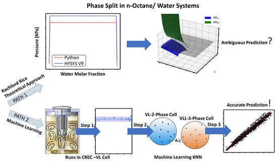
When applying the Newton–Raphson method (Equations (23)–(27)) using an initial estimate within the set boundaries (as presented in the following section), such as ${\beta }_{sup}^V=0.4$ and ${\beta }_{sup}^W=0.2$, for the water/PASN, employing SRKKD EoS model and Python, the result is ${\beta }^V=0.10004025$ and ${\beta }^W=0.44494793$ root with four iterations only. In this respect, the HYSYS V9 results in this case were ${\beta }^V=0.1$ and ${\beta }^W=0.4449395$, with the difference being much lower than 0.1%. In contrast and as expected, for the water/n-octane system, the calculation reaches the 10,000 maximum number of iterations with the obtained results not having physical meaning: ${\beta }^V=-10.9198$ and ${\beta }^W=2.6645\ast {10}^{-15}$.

Given the above, the function $F\left(\beta \right)$(Equation (49)) for the water/PASN mixture was minimized using different methods within the minimize functions available in the Python Optimize library. Tolerance was set in the 10⁻⁸ range, with the percentage of difference for the calculated $\beta$ values being lower than 0.3%.

Table 1. Results for water/PASN system using different methods for the minimize function of Scipy-Optimize package for Python.

Initial Estimate	Method	Result	% Difference
$\beta =\left[\begin{array}{cc}0.4& 0.2\end{array}\right]$	Constrained Optimization BY Linear Approximation (COBYLA)	$\beta =\left[\begin{array}{cc}0.10004048& 0.44494783\end{array}\right]$	$\left[\begin{array}{cc}0.04\%& 0.0019\%\end{array}\right]$
$\beta =\left[\begin{array}{cc}0.4& 0.2\end{array}\right]$	Sequential Least Squares Programming (SLSQP)	$\beta =\left[\begin{array}{cc}0.10004144& 0.44494715\end{array}\right]$	$\left[\begin{array}{cc}0.04\%& 0.0017\%\end{array}\right]$
$\beta =\left[\begin{array}{cc}0.4& 0.2\end{array}\right]$	trust-constr	$\beta =\left[\begin{array}{cc}0.09995574& 0.44541656\end{array}\right]$	$\left[\begin{array}{cc}0.04\%& 0.1072\%\end{array}\right]$
$\beta =\left[\begin{array}{cc}0.9& 0.1\end{array}\right]$	Constrained Optimization BY Linear Approximation (COBYLA)	$\beta =\left[\begin{array}{cc}0.1000405& 0.44494781\end{array}\right]$	$\left[\begin{array}{cc}0.04\%& 0.0019\%\end{array}\right]$
$\beta =\left[\begin{array}{cc}0.9& 0.1\end{array}\right]$	Sequential Least Squares Programming (SLSQP)	$\beta =\left[\begin{array}{cc}0.09993294& 0.44500976\end{array}\right]$	$\left[\begin{array}{cc}0.07\%& 0.016\%\end{array}\right]$
$\beta =\left[\begin{array}{cc}0.9& 0.1\end{array}\right]$	trust-constr	$\beta =\left[\begin{array}{cc}0.09976697& 0.44642034\end{array}\right]$	$\left[\begin{array}{cc}0.23\%& 0.32\%\end{array}\right]$

reports the various methods tested. Best results were obtained using the constrained optimization by linear approximation (COBYLA) method.

However, in spite of this, none of the considered methods led us to meaningful physical solutions for water/n-octane blends, as reported in

Table 2. Results for water/n-octane system using different methods for the minimize function of Scipy-Optimize package for Python.

Initial Estimate	Method	Result
$\beta =\left[\begin{array}{cc}0.4& 0.2\end{array}\right]$	Constrained Optimization BY Linear Approximation (COBYLA)	$\beta =\left[\begin{array}{cc}-0.1780& 0.6150\end{array}\right]$
$\beta =\left[\begin{array}{cc}0.4& 0.2\end{array}\right]$	Sequential Least Squares Programming (SLSQP)	$\beta =\left[\begin{array}{cc}0.4146& 0.2220\end{array}\right]$
$\beta =\left[\begin{array}{cc}0.4& 0.2\end{array}\right]$	trust-constr	$\beta =\left[\begin{array}{cc}0.4150& 0.2224\end{array}\right]$
$\beta =\left[\begin{array}{cc}0.9& 0.1\end{array}\right]$	Constrained Optimization BY Linear Approximation (COBYLA)	$\beta =\left[\begin{array}{cc}-0.0142& 0.5063\end{array}\right]$
$\beta =\left[\begin{array}{cc}0.9& 0.1\end{array}\right]$	Sequential Least Squares Programming (SLSQP)	$\beta =\left[\begin{array}{cc}0.8080& -0.0388\end{array}\right]$
$\beta =\left[\begin{array}{cc}0.9& 0.1\end{array}\right]$	trust-constr	$\beta =\left[\begin{array}{cc}0.8086& -0.0377\end{array}\right]$

. Not even a genetic algorithm was able to numerically solve this case, arriving at a result of $\beta =\left[\begin{array}{cc}-20.7& 14.2\end{array}\right]$. Additional explanations of this matter are described in Section 4.4.

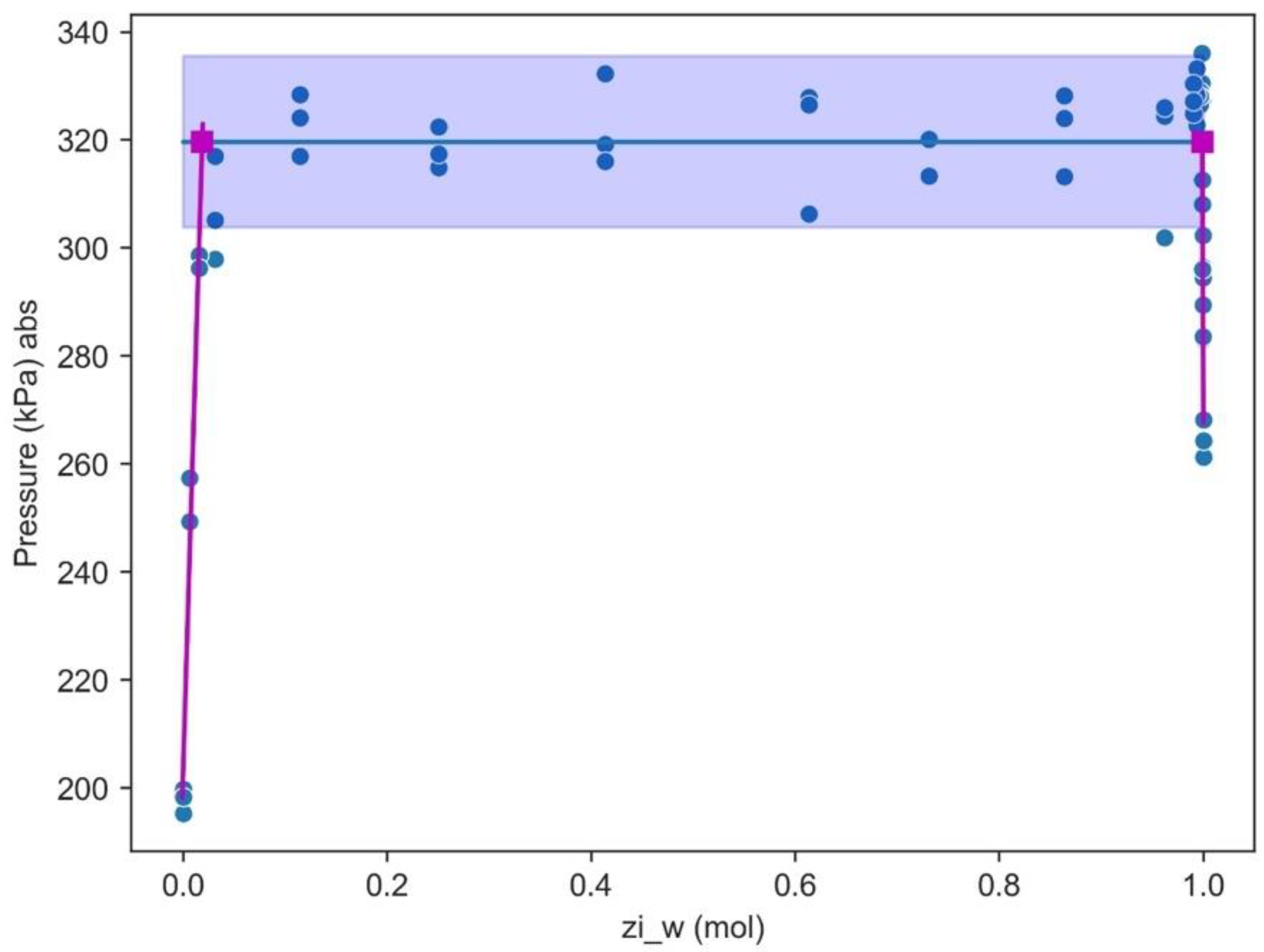
Regarding the VLLE for water/PASN, it can be calculated accordingly, as reported in

Table 3. Pressure calculation results for water/PASN system in VLLE region (no air).

Conditions	Python Results (kPa)	HYSYS V9 Results (kPa)	Difference (%)
T = 80 °C	86.10	91.53	6.31%
Zw = 0.5
T = 80 °C	86.10	91.53	6.31%
Zw = 0.1
T = 80 °C	86.10	91.53	6.31%
Zw = 0.9
T = 110 °C	242.55	254.41	4.89%
Zw = 0.5
T = 110 °C	242.55	254.41	4.89%
Zw = 0.1
T = 110 °C	242.55	254.41	4.89%
Zw = 0.9

. In this case, the bubble pressure (${\beta }^V=0$), which is of interest for this research, can be calculated using both Python and Hysis V9.

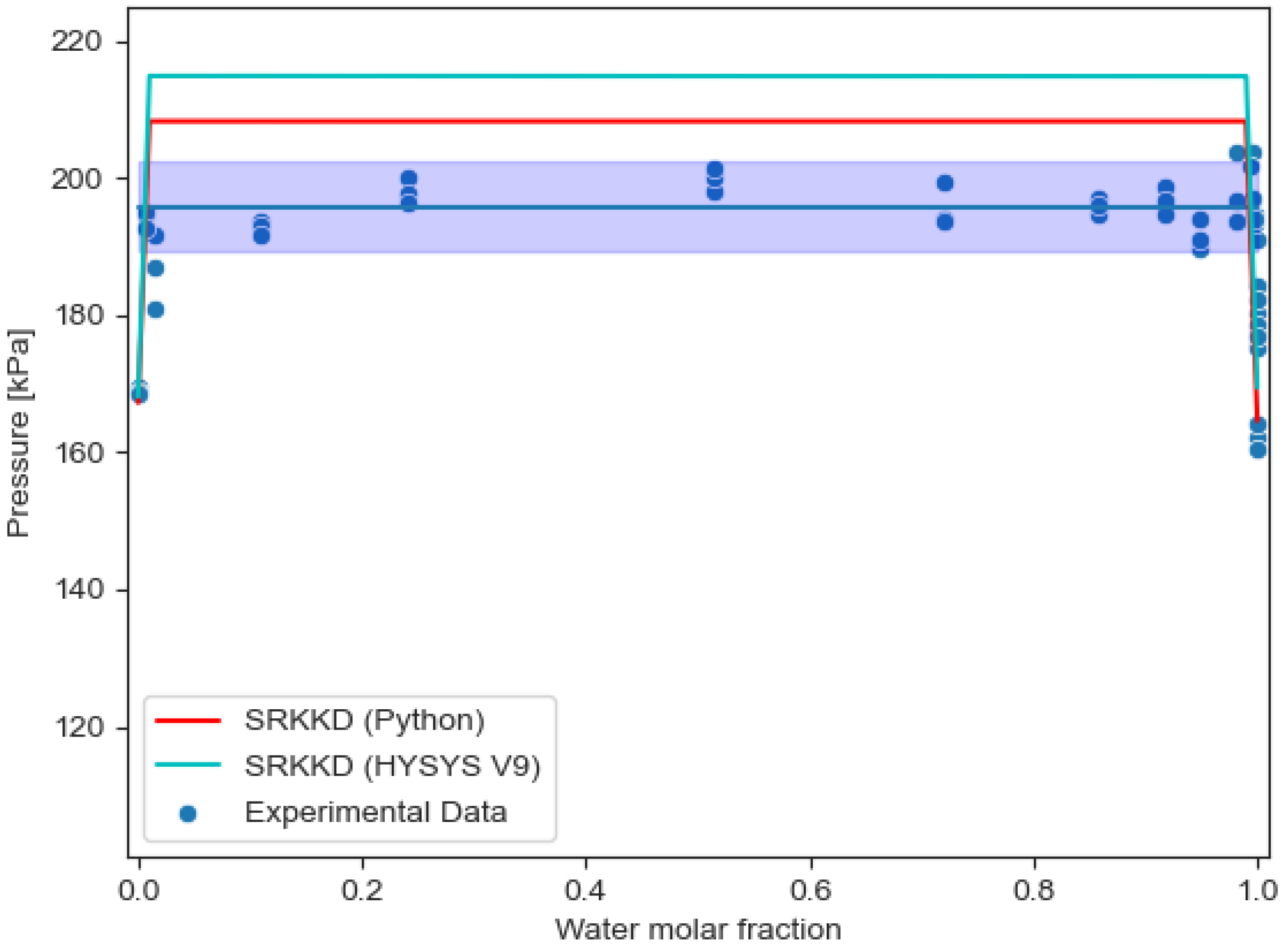
However, when comparing VLLE results from HYSYS V9 and results from SRKKD EoS implemented with Python, the described Python algorithm for water/PASN works better to calculate pressure results than HYSYS V9, as shown in Figure 5 and Figure 6, with SRKKD EoS implemented with Python achieving better agreement with experimental data from the CRE VL-Cell.

On the other hand, in the case of water/n-octane blends, the described algorithm presents convergence problems. To describe these issues, it is important to establish how the numerical Rachford–Rice equations (Equations (17)–(19)) influence these types of iterative calculations for both water/n-octane and water/PASN mixtures. To address this matter, the following section evaluates the approach proposed by Li and Firoozabadi [29] and the boundaries set by Okuno et al. [20].

4.4. Issues with Constant-K Solution Calculations

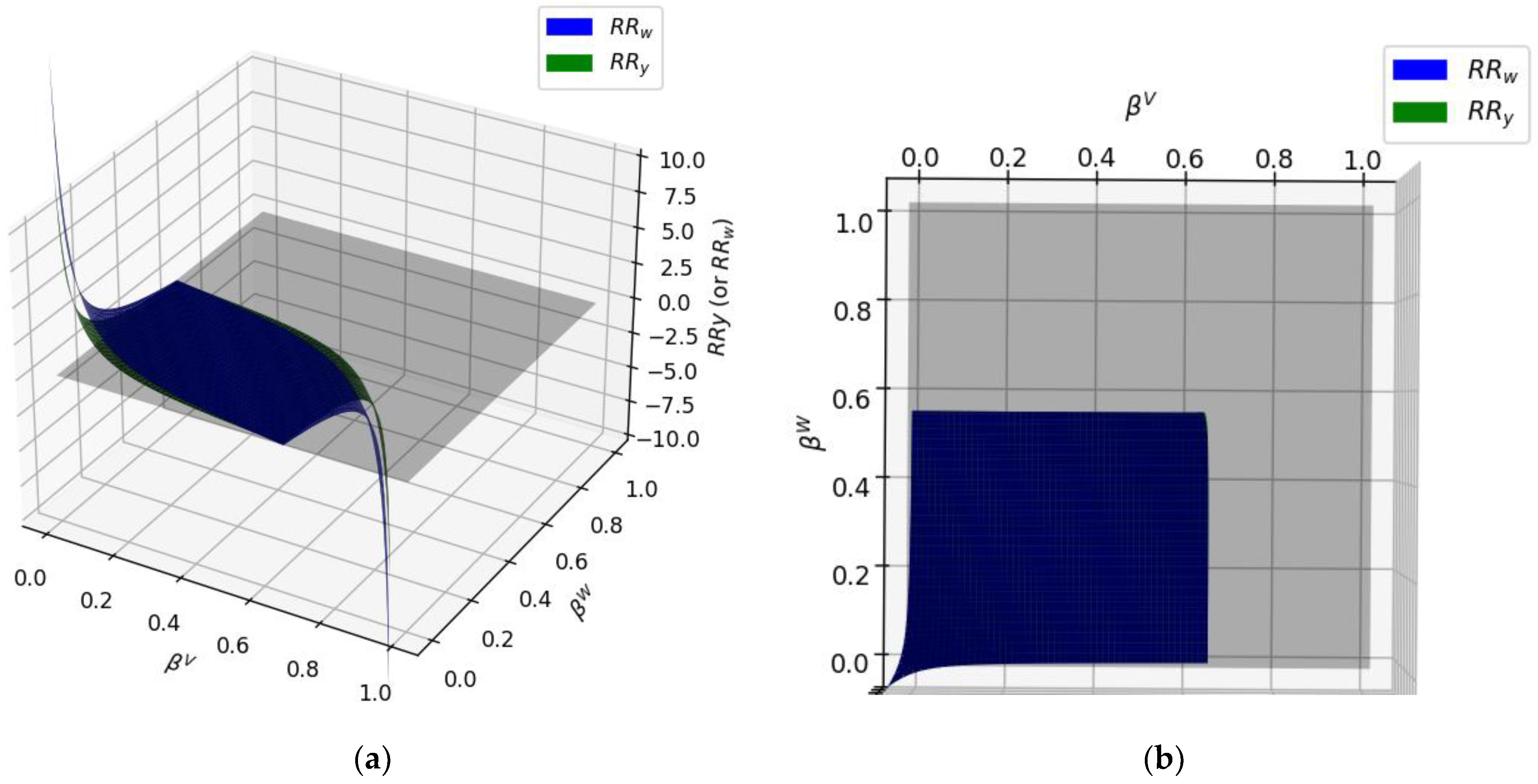
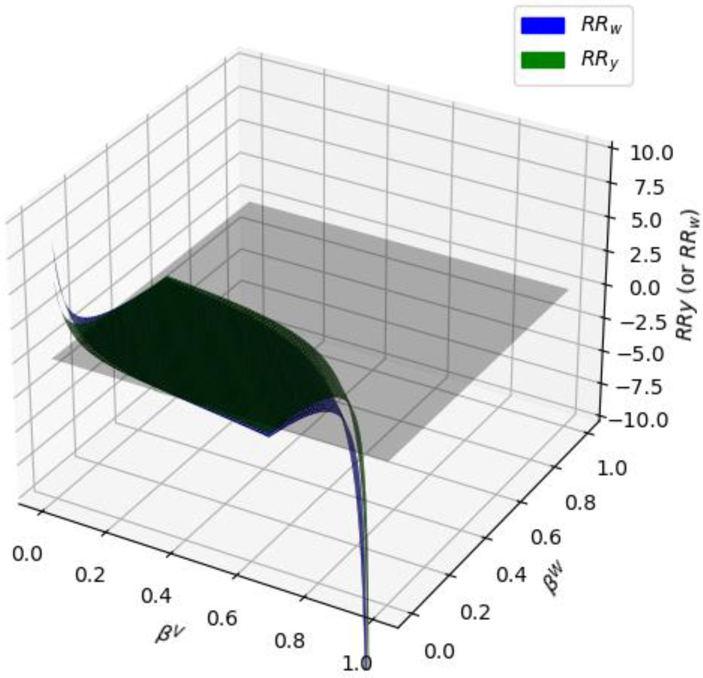
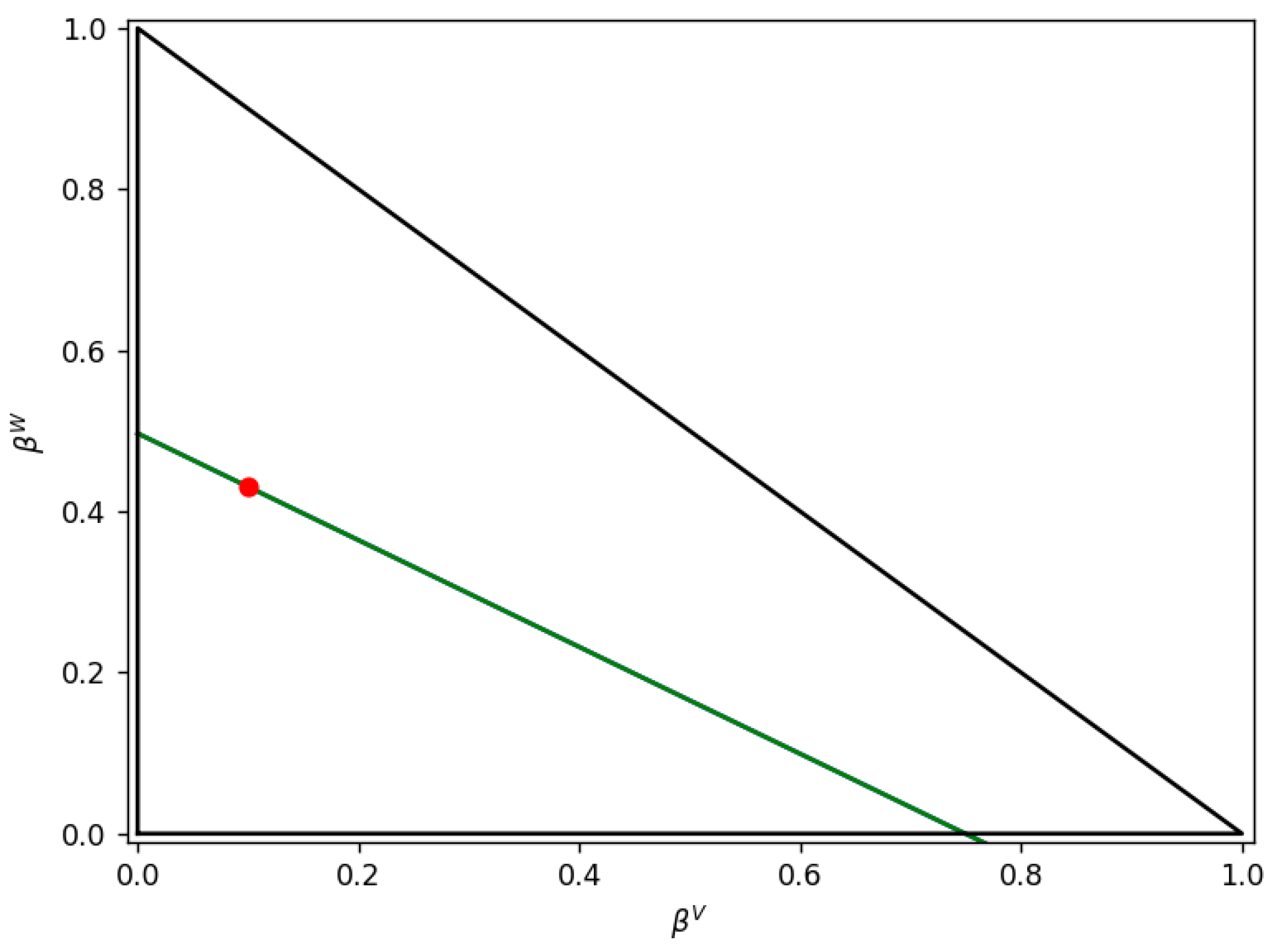
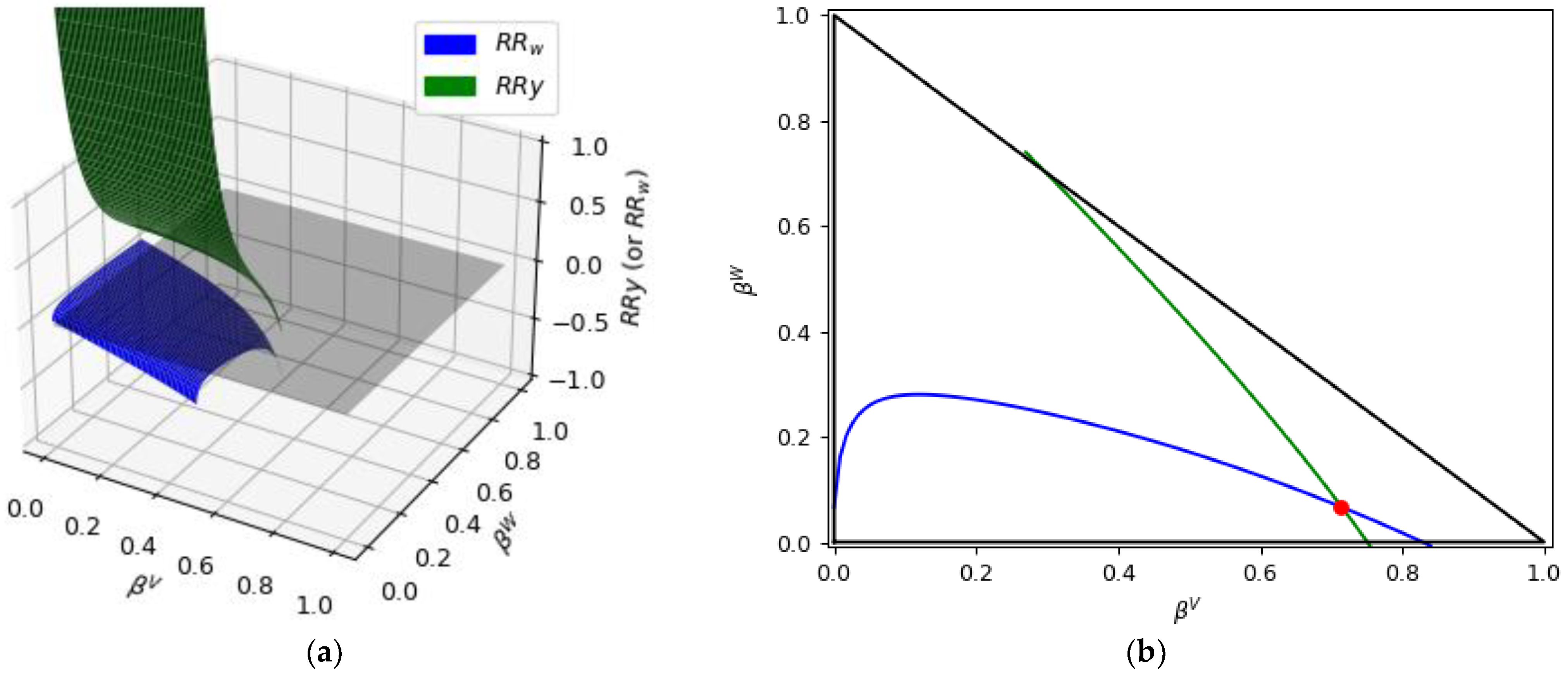
Li and Firoozabadi [29] reported some examples of how $R{R}_y$ and $R{R}_w$ surfaces (Rachford–Rice surfaces) change, whereas ${\beta }^V$ and ${\beta }^w$ are varied, with ${\beta }^V$ and ${\beta }^w$ parameters representing the vapor and water fraction, respectively. A display of one of the examples reported by Li and Firoozabadi for a general case [29] is shown in Figure 7 for $R{R}_y$ and $R{R}_w$ intersecting the z = 0 plane.

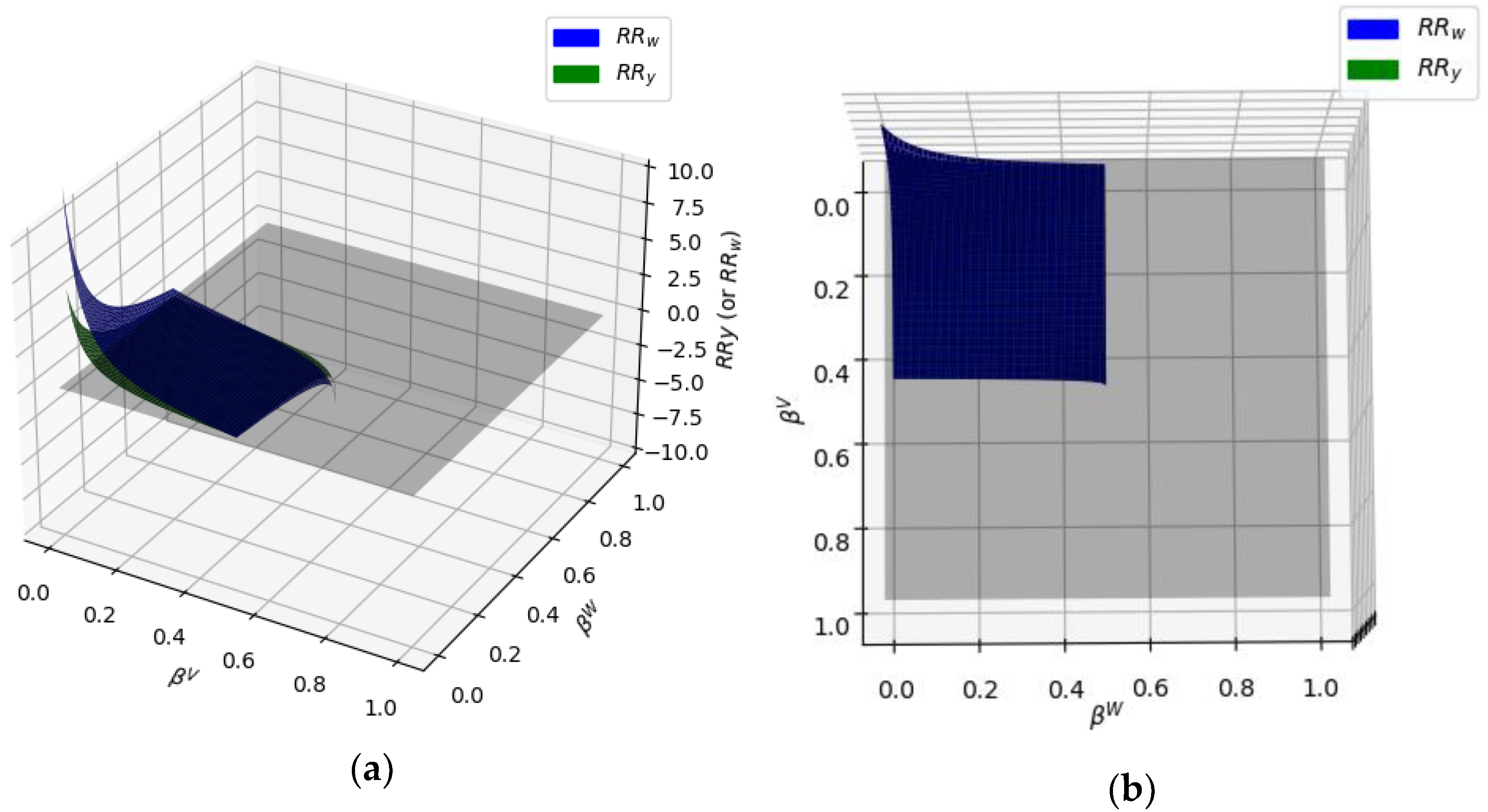
The triangle defined in Figure 7a by the vertices (0,1), (0, 0), and (1, 0) represents the solution domain [29], with the solution at $R{R}_y=0$ and $R{R}_w=0$ plane shown with a red dot.

In this regard, if one attempts to develop a similar Python-based calculation for an octane/water blend “constant-K” flash, one can observe that it is not possible to obtain a converging iterative solution. This is also true for a wide range of octane in water concentrations in the 0.5–99.75 wt.% range.

As a result, to provide a sound explanation of the findings, the following steps were followed:

(a)

The first step involves the SRKKD EoS model and HYSYS V9 with “constant-K” flash simulations. Equilibrium constants are approximated on this basis and used later for a thorough analysis of Rachford–Rice equations.

(b)

The second step considers a “constant-K” flash calculation using the equilibrium constant calculated in step 1. This helps to provide a good understanding of how the Rachford–Rice equations perform in such hydrocarbon/water mixtures.

4.4.1. Octane–Water Blends

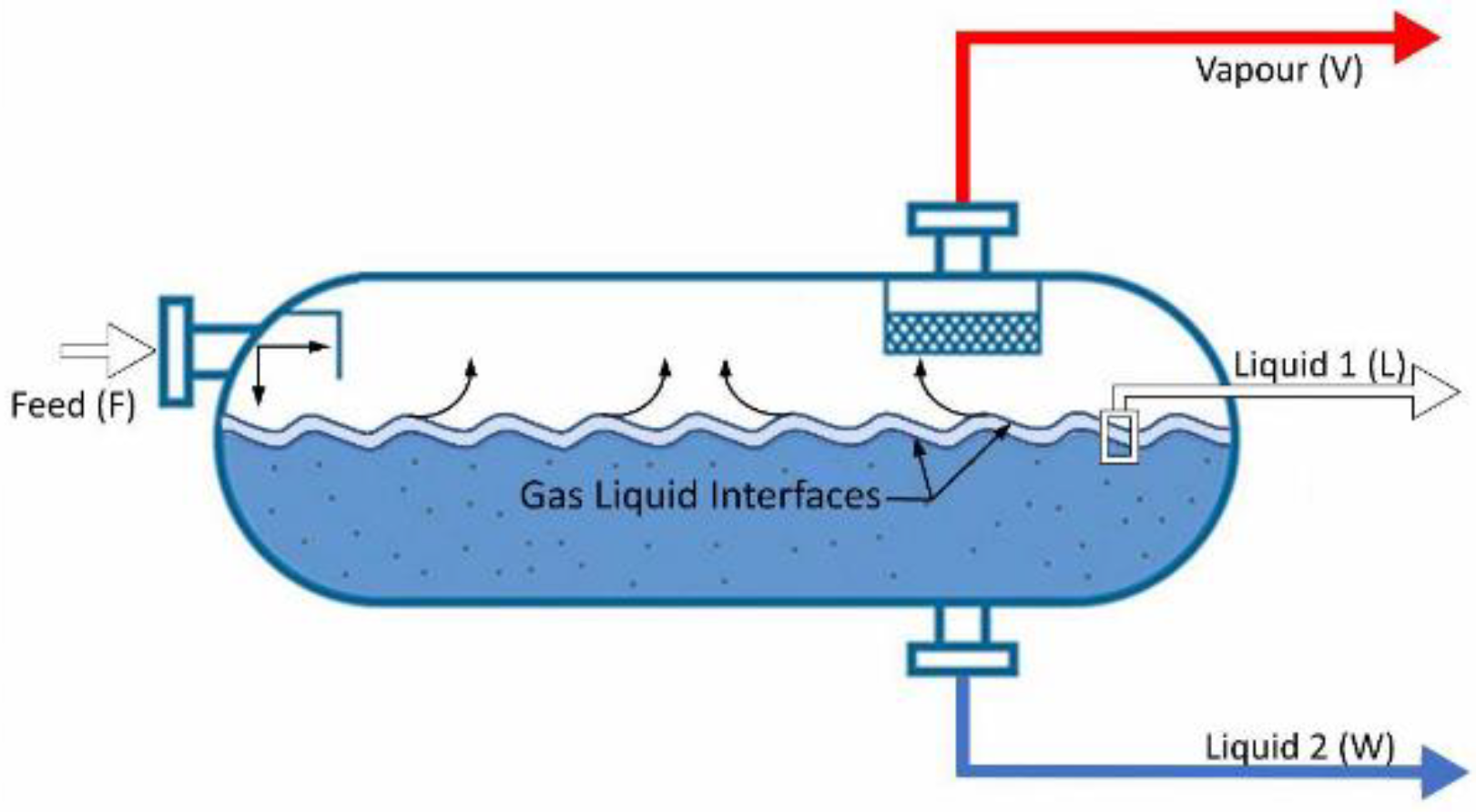
To illustrate the calculations, a three-phase separator was specified in HYSYS V9 feeding a 100 kgmol/h blend with a 50% mol water/50% mol n-octane mixture for the first step. Working conditions for this three-phase separator were T = 80 °C and a vapor fraction of 0.1. In this case, the presence of air was not considered. Results obtained are reported in

Table 4. HYSYS V9 results for three-phase flash calculations at T = 80 °C using SRKKD.

		Molar Fraction
	Molar Flow (kgmol/h)	Water	n-Octane
Feed	100.00	0.5	0.5
Hydrocarbon Phase	46.94	6.09 × 10−3	0.9939
Aqueous Phase	43.06	$\approx$1.0	1.20 × 10−6
Vapor	10.00	0.6651	0.3349

.

In developing the second calculation step, using the $K_i^V$ and $K_i^W$ constants obtained from HYSYS V9 in Python, the RR_y and RR_w values were in a low-level range, as shown in Figure 8a. The values of ${\beta }^V$ and ${\beta }^w$ also changed in a restricted domain. Furthermore, if the ${\beta }^V$ value was higher than 0.63 or ${\beta }^w$ was higher than 0.58, the solution for $R{R}_y$ and $R{R}_w$ did not converge.

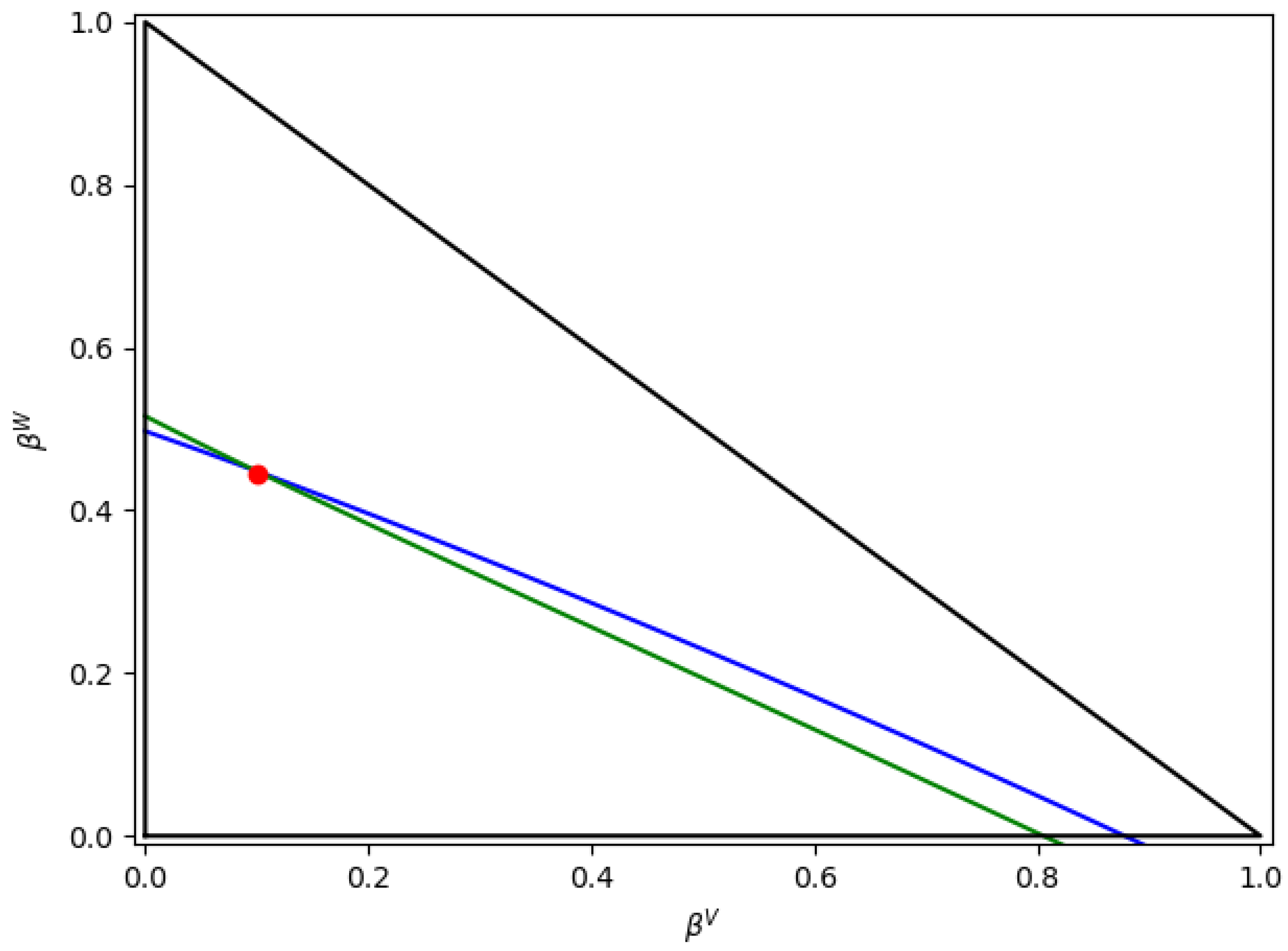
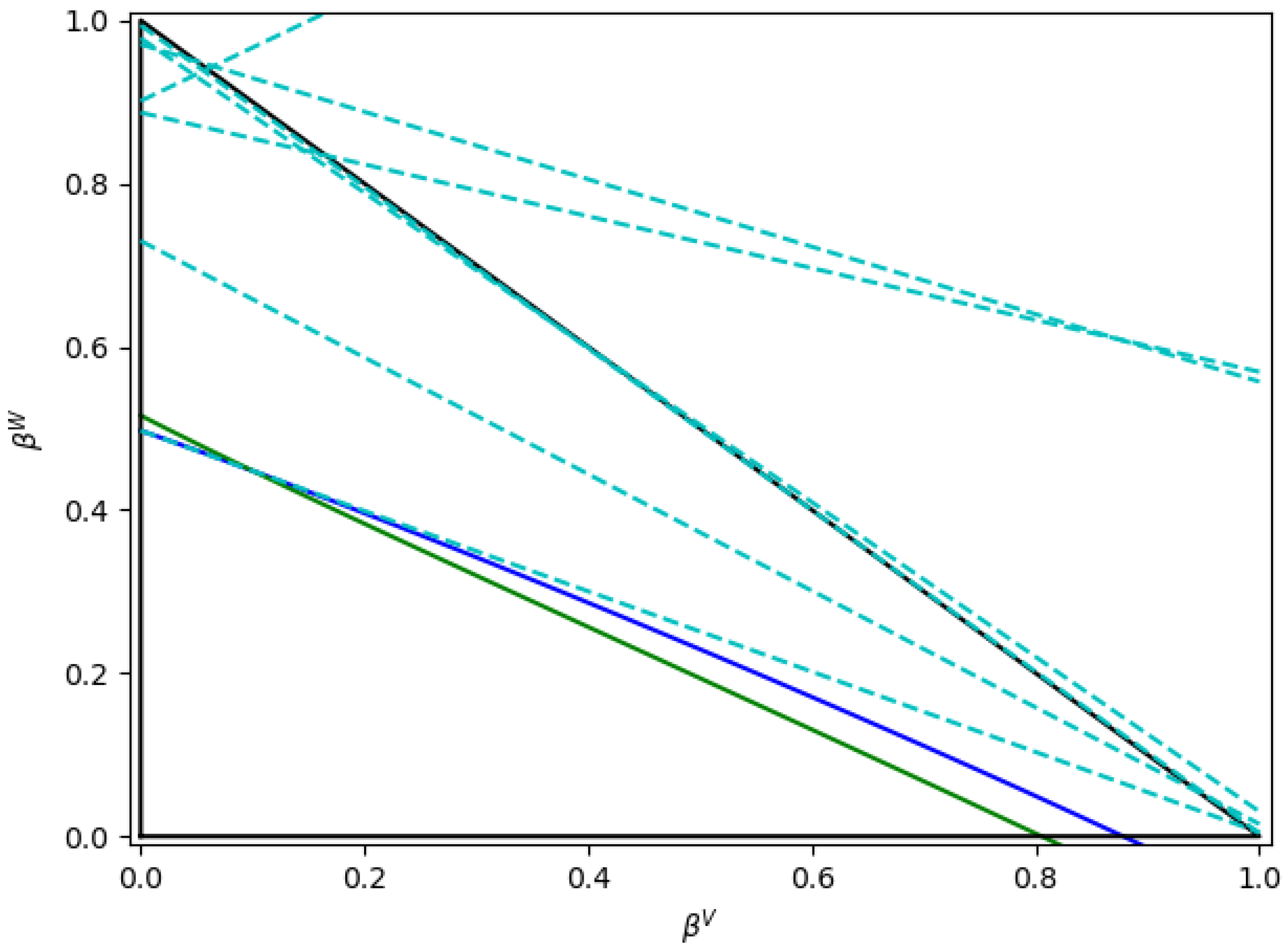
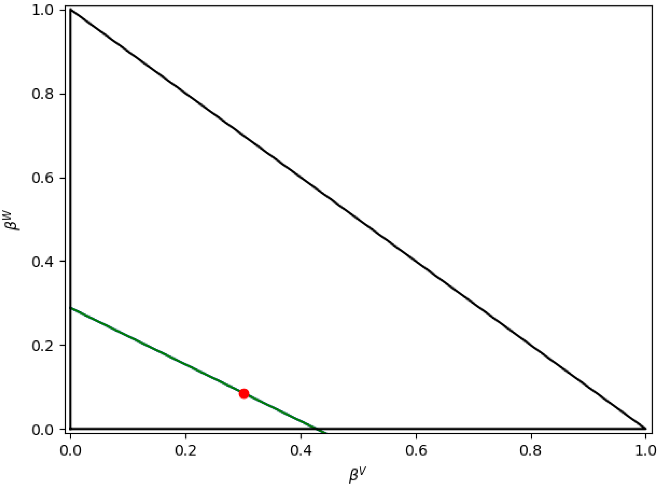
Additionally, when RR_y and RR_w were considered at z = 0, the obtained ${\beta }^w$ for different values of ${\beta }^V$ led to two parallel and z = 0 plane-superimposed RR_y and RR_w straight lines, as shown in Figure 9. In contrast, an HYSYS V9 solution was obtained, as identified with a red dot in Figure 9.

As a result of this and under these conditions, one can understand why the iterative calculations trying to find an intersection of the RR_y and RR_w lines fail and the “constant-K” solution remains unknown.

Regarding these results, Haugen and Firoozabadi [24] advanced that algorithms of this type solving RR equations can fail when the lines at RR_y = 0 and RR_w = 0 are parallel in the domain of interest. In this respect, these authors designated these conditions as the result of a “bicritical point” where two of the phases have very similar compositions. They identified three different kinds of “bicritical regions” [24]: (i) $K_i^V\approx 1$, (ii) $K_i^W\approx 1$ or (iii), and $K_i^V\approx K_i^W$. In this case, the K values for water/n-octane mixtures are as follows: $K_i^V=\left[{1.092510}^2, {3.369210}^{-1}\right]$ and $K_i^W=\left[{1.642610}^2, {1.210510}^{-6}\right]$. As a result and given the conditions considered involving $K_i^V\approx K_i^W$, they could be considered in partial agreement with case (iv) from the Haugen and Firoozabadi criteria [24].

For different temperatures (in this case, 110 °C) (

Table 5. HYSYS V9 results for three-phase flash calculations at T = 100 °C using SRKKD.

		Molar Fraction
	Molar Flow (kgmol/h)	Water	n-Octane
Feed	100.00	0.3	0.7
Hydrocarbon Phase	61.38	1.60 × 10−2	0.9840
Aqueous Phase	8.62	$\approx$1.0	2.06 × 10−6
Vapor	30.00	0.6799	0.3201

), the behavior of n-octane/water mixtures displays similar calculation challenges, as can be observed in Figure 10 and Figure 11.

Haugen et al. (2011) [24] described that the non-converging lines problem leads to a very large number of iterations, with the numerical solution becoming unacceptably expensive.

Thus, in the case of octane/water mixtures, the described $\mathrm{shape}\mathrm{of}\mathrm{the} R{R}_y$ and $R{R}_w$ surfaces make it very challenging for a proposed algorithm, such as the SRKKD EoS model with Python algorithm, to converge towards a “constant-K” flash solution.

4.4.2. PASN/Water Blends

In contrast with the “non-convergence” results described in Section 4.3 and Section 4.4.1 for n-octane/water blends, the PASN/water mixtures evaluated with the SRKKD EoS model with Python can provide consistent “constant-K” flash-convergent simulations. This is the case when performing flash calculations for a 50%mole water/PASN mixture. Results after convergence are presented in

Table 6. PASN/water mixture three-phase flash calculations at T = 80 °C and P = 83.16 kPa using SRKKD model, the Rachford–Rice equations and the Python calculations of the present study.

		Molar Fraction
	Molar Flow (kgmol/h)	Water	n-Hexane	n-Heptane	n-Octane	n-Decane	Toluene	n-Dodecane
Feed (Water)	50.00	1	0	0	0	0	0	0
Feed (PASN)	50.00	0	0.11939808	0.2259054	0.540451	4.34 × 10−2	5.88 × 10−2	1.21 × 10−2
Hydrocarbon Phase	45.51	5.48 × 10−3	0.0967	0.2171	0.5623	4.75 × 10−2	5.75 × 10−2	1.33 × 10−2
Aqueous Phase	44.49	$\approx$1.00	5.80 × 10−17	5.11 × 10−19	2.74 × 10−21	8.65 × 10−28	2.70 × 10−12	1.47 × 10−34
Vapor	10.00	0.4951	0.1599	0.1481	0.1604	2.47 × 10−3	3.37 × 10−2	1.32 × 10−4

.

Figure 12 reports the calculated RR_y and RR_w, using K_i^V and K_i^W from the SRKKD model using the Python calculations. In this case, values of ${\beta }^V$ and ${\beta }^W$ are smaller than 0.5, providing converging numerical solutions in all cases.

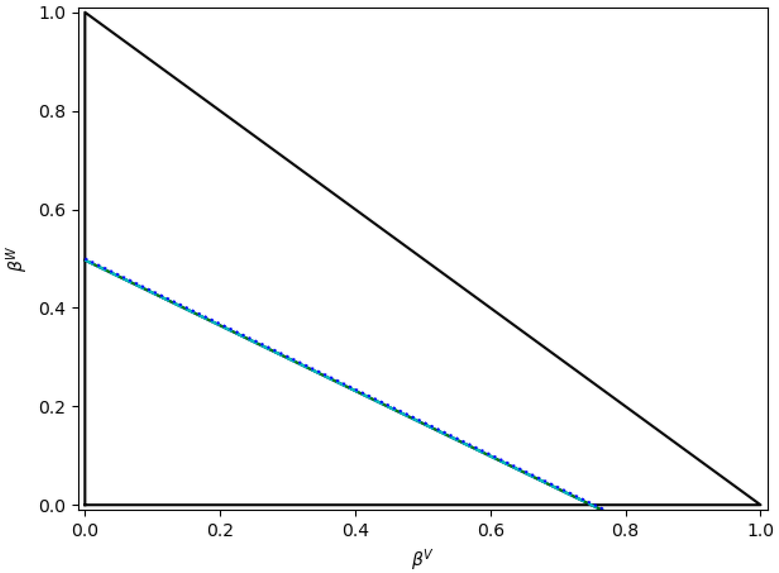
Figure 13 further describes the “constant-K” flash solution for the $R{R}_y=0$ and $R{R}_w=0$ lines, displaying the numerical ${\beta }^V$ and ${\beta }^W$ solutions with convergence assured.

4.4.3. Boundary Conditions

Regarding the boundary conditions, if one considers the water/n-octane mixture with K_i approximated by HYSYS V9 (Figure 11), the boundary conditions proposed by Okuno et al. [20] result in Equations (54) and (55), with the hyperplanes superimposed to the lines for $R{R}_y=0$ and $R{R}_w=0$, as presented in Figure 14.

$$-108.2527{\beta }^V-163.2577{\beta }^W\le -81.1289$$

(54)

$$0.6631{\beta }^V+{\beta }^W\le 0.5$$

(55)

Furthermore, in applying the boundary conditions proposed by Okuno et al. [20] for the water/PASN blend, the hyperplanes related to Equations (56)–(62) can be represented as in Figure 15.

$$-89.43 {\beta }^V-181.62 {\beta }^W\le -90.31$$

(56)

$$-0.6535 {\beta }^V+{\beta }^W\le 0.9013$$

(57)

$$0.3178 {\beta }^V+{\beta }^W\le 0.8870$$

(58)

$$0.7147 {\beta }^V+{\beta }^W\le 0.7297$$

(59)

$$0.9479 {\beta }^V+{\beta }^W\le 0.9783$$

(60)

$$0.9901 {\beta }^V+{\beta }^W\le 0.9940$$

(61)

$$0.4134{\beta }^V+{\beta }^W\le 0.9706$$

(62)

4.4.4. Remarks

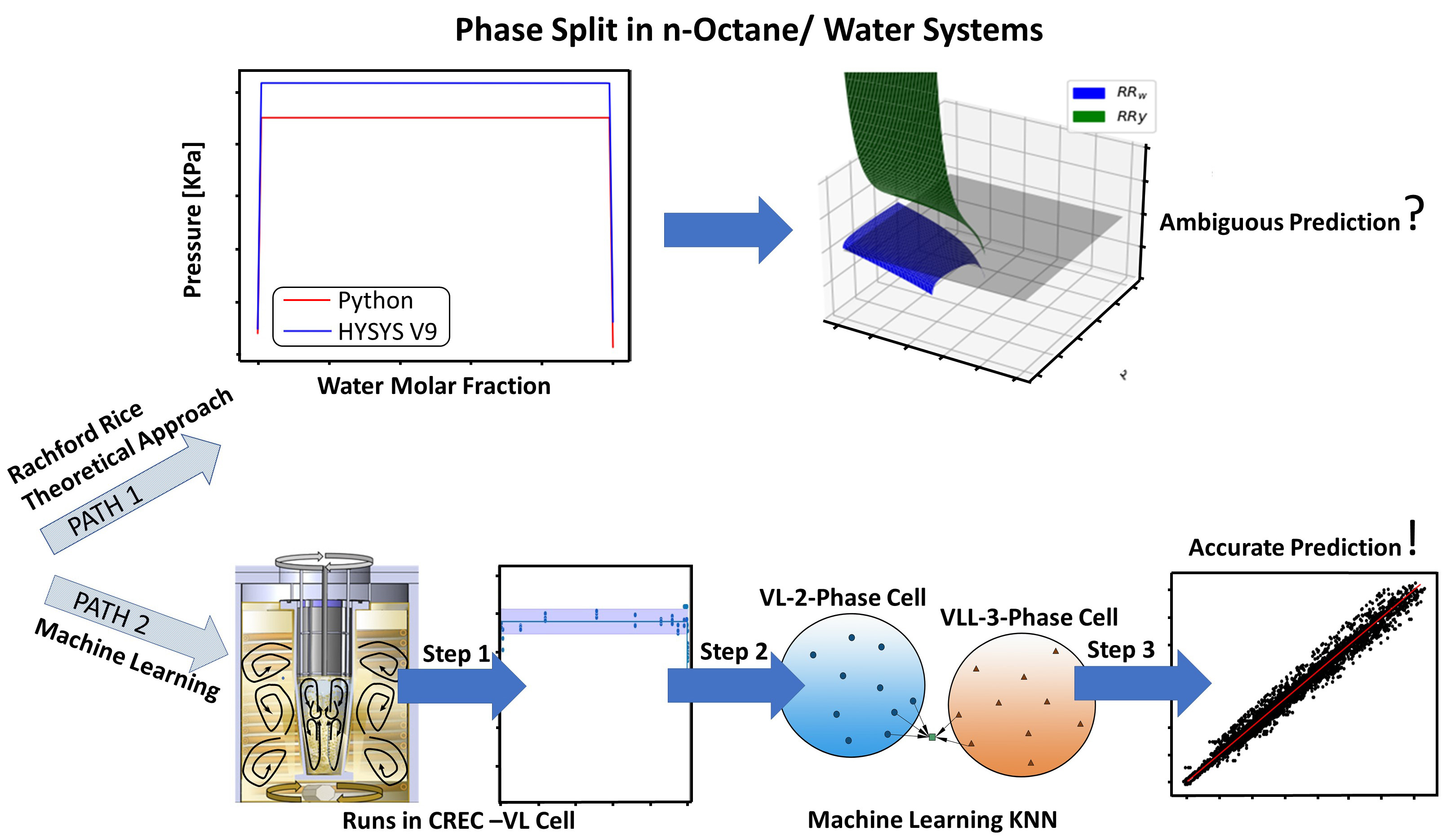
On the basis of results from “constant-K” flash calculations for n-octane/water and PASN/water blends, one can conclude that the composition of hydrocarbon/water blends is a key factor in allowing for a viable numerical calculation using the Rachford–Rice equations. Thus, to address possible calculation uncertainty and ambiguity resulting for octane/water blends, an alternate methodology to calculate the molar fractions and mixture pressure is proposed in the upcoming sections.

4.5. Liquid-Phase K-Values from Experimental Data for Water/n-Octane Mixtures

As discussed in the previous sections, the initial guess for K values affects the convergence of the flash calculation algorithm (Figure 4). Usually, Wilson correlation [30] (Equation (63)) is used as a first approximation for the K value in the hydrocarbon phase. For the K values in the water phase, Connolly et al. [1] suggested values based on the initial feed, as presented in Equation (64).

$$\ln K_i^{Wilson}=\ln \frac{P_i^C}{P}+5.373\left(1-{\omega }_i\right)\left(1-\frac{T_i^C}{T}\right)$$

(63)

$$K_i^{H_{2}O}=\frac{0.999}{z_i}$$

(64)

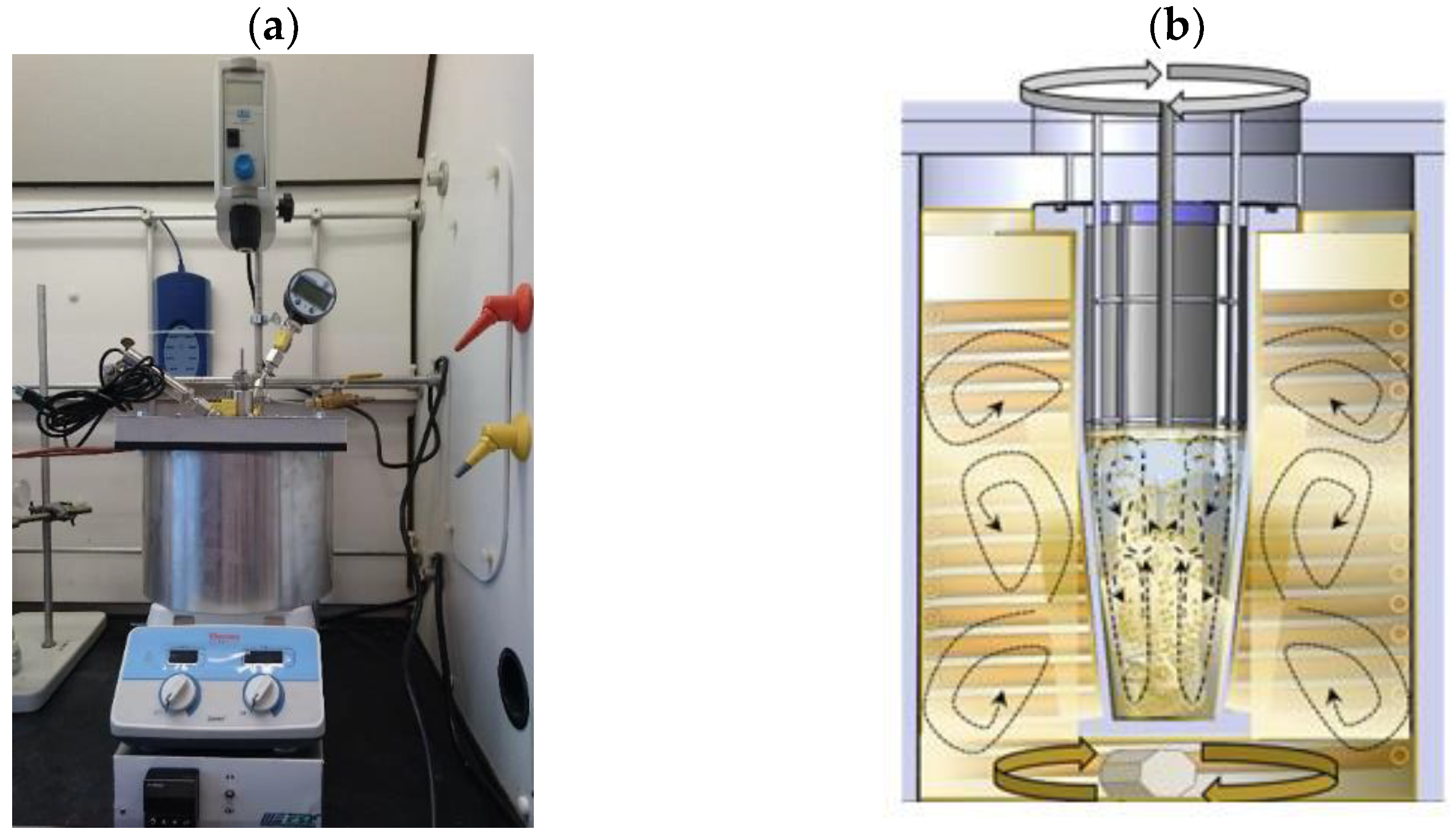
In this sense, another advantage of the CREC VL-Cell developed by CREC researchers is that it allows one to determine the solubility values based on the VLLE data obtained. The transition from the three-phase and two-phase regions defines the solubility limit. Figure 16 presents the solubility limit regions for a water/n-octane mixture at 110 °C. This region is characterized by the transition from three phases to two phases.

The applicability of the CREC-VL-Cell for establishing solubility and solubility limits is not restricted to any type of hydrocarbon/water blend. Thus, the CREC-VL-Cell can be of special value in dealing with hydrocarbon/water blends involving intrinsic convergence uncertainties observed by octane–water mixtures while using the Rachford–Rice equations (refer to Section 4.4).

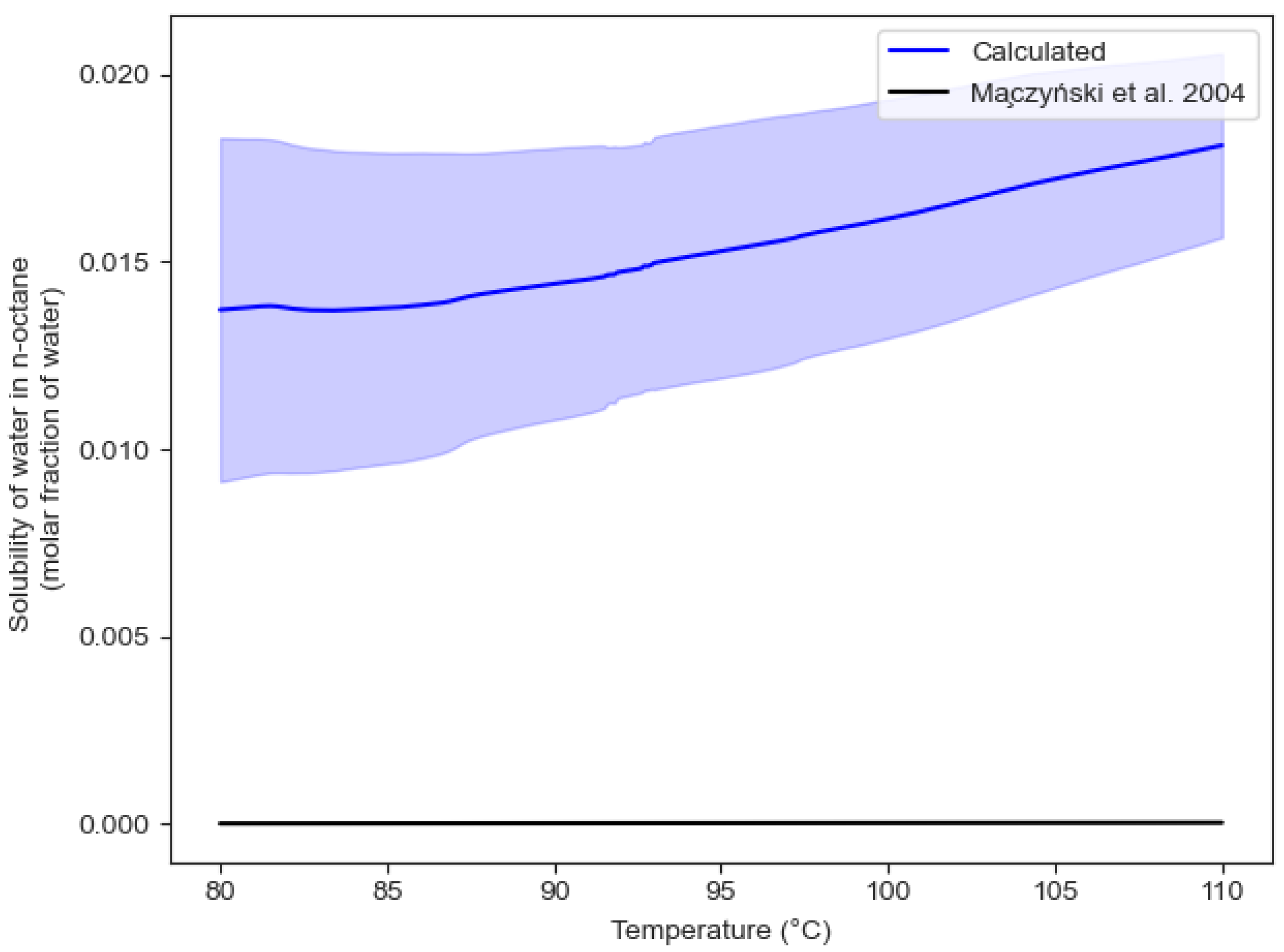
Figure 17 shows that the solubility limit for an octane/water blend can be calculated from the intersection between the lines that define the three-phase and two-phase domain. The calculated solubilities at 110 °C are $x_w^L=0.01810534\pm 2.5\times {10}^{-3}$ and $x_{oct}^W=0.00084875\pm 2.6\times {10}^{-4}$, considering the 95% confidence interval defined by the blue region. Although the solubility of water in n-octane is in close agreement with $x_w^L=0.016$ calculated, the value using HYSYS V9 with SRKKD EoS and Rachford–Rice equations yields a solubility for n-octane in water two orders of magnitude higher compared with the $x_{oct}^W=2.06\times {10}^{-6}$ Hysis V9-predicted value.

As a result, once the solubility values are obtained from the CREC-VL-Cell, it is possible to calculate $K_i^W=\frac{x_i^W}{x_i^L}$ water-phase constants as $K_i^W=\left[\begin{array}{cc}55.185& 8.64\times {10}^{-4}\end{array}\right]$. Furthermore, for the vapor phase species at equilibrium, one can obtain an approximative value using $y_i=\raisebox{1ex}{$\frac{x_i^L{\varphi }_i^L}{{\varphi }_i^V}$}\!\left/ \!\raisebox{-1ex}{${{\displaystyle \sum }}_i^N\frac{x_i^L{\varphi }_i^L}{{\varphi }_i^V}$}\right.$ and $K_i^V=\frac{y_i}{x_i^L}$. Assuming the vapor phase behaves as an ideal gas, then ${\varphi }_i^V \approx 1$, and the obtained results are $y_w\approx 0.7347\pm 2.38\times {10}^{-2}$ and $K_i^V=\left[\begin{array}{cc}40.5772& 0.2702\end{array}\right]$.

The mean value obtained has a 16.04% difference from the value predicted by HYSYS V9 ($y_w\approx 0.6799$). However, the HYSYS V9 value is within the range of the 95% confidence interval. Figure 18 and Figure 19 report the observed solubilities of water in n-octane and n-octane in water, respectively, as determined in the CREC VL-Cell and compared with the values reported by Maczynski et al. (2004) [31] for both water in n-octane and n-octane in water.

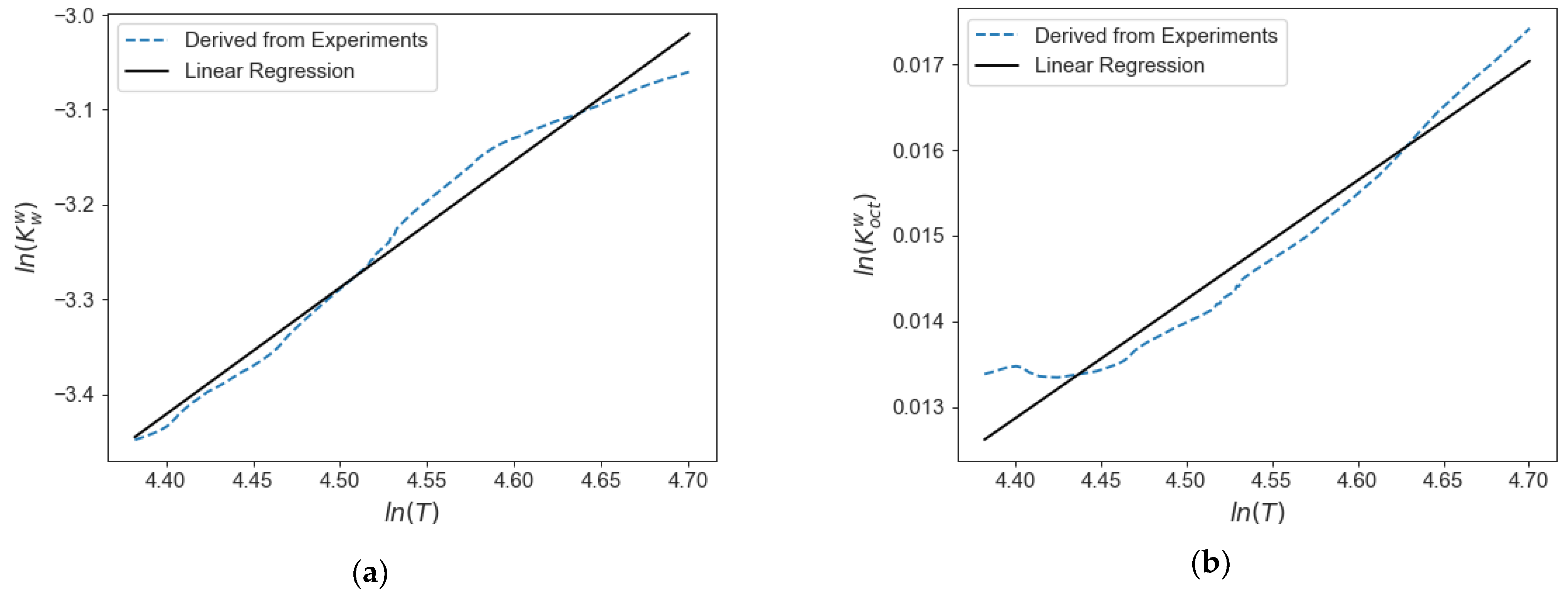
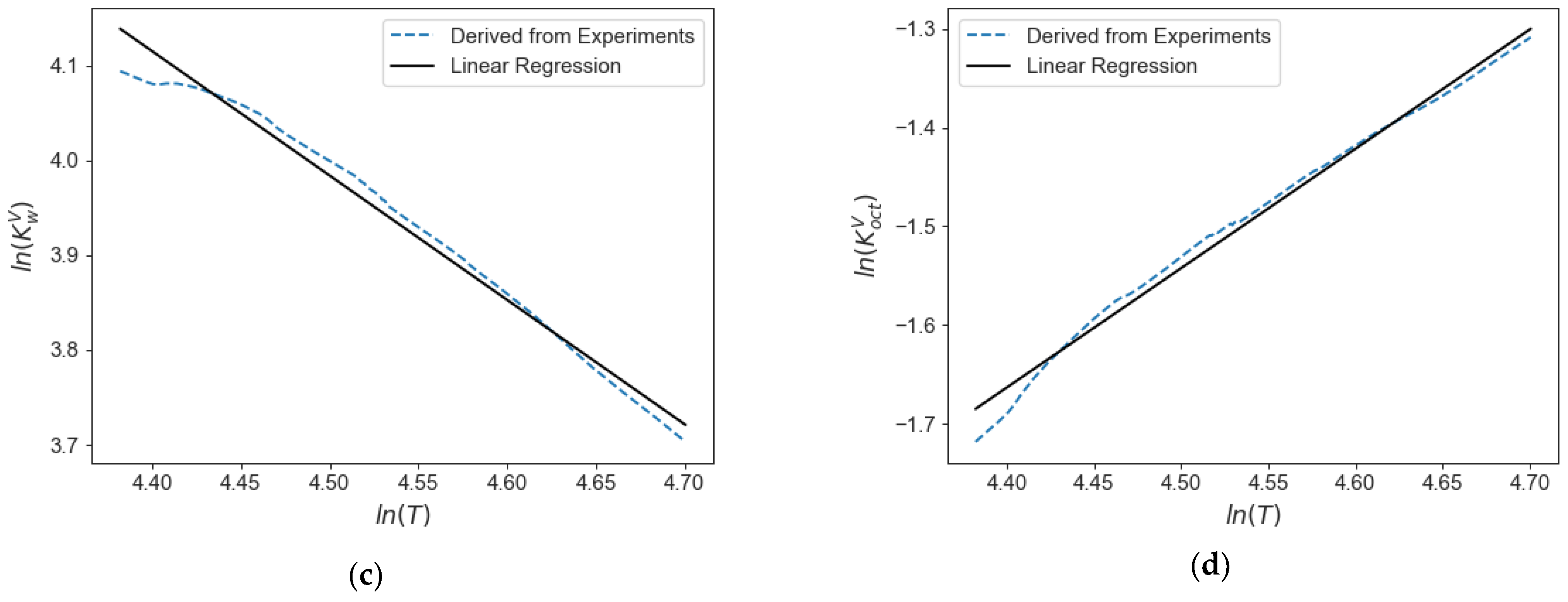
Furthermore, on the basis of the experimental data obtained in the CREC-VL-Cell, a correlation to obtain the K values for water/octane mixtures in the temperature range of interest and low pressure (1–3 atm) is proposed. This correlation is given by the following Equation (65), with the constants involved reported in

Table 7. Constants for K-value correlation of water/n-octane system.

	Compound	m	b	R2
$K_i^W$	Water	1.3366	−9.3022	0.9786
$K_i^W$	Octane	0.01390	−0.0483	0.9563
$K_i^V$	Water	−1.3113	9.8849	0.9851
$K_i^V$	Octane	1.2099	−6.9870	0.9910

. A comparison with calculated values from experimental results is also reported in Figure 20, showing the adequate fitting of the experimental values by this correlation.

$$\ln K_i^p=m\ln T+b$$

(65)

Given the observed differences with the experimental points reported in Figure 6 and obtained in the CREC-VL-Cell, it is important to provide a more precise methodology to calculate the pressures at VLLE, accounting for the uncertainties related to the experimental values. This will be discussed in the following section.

4.6. Machine Learning Approach

As shown in the previous sections of this work (Section 4.1, Section 4.2, Section 4.3, Section 4.4, Section 4.5), traditional thermodynamic models for multiphase systems based on Rachford–Rice equations overpredict vapor pressure in cases unable to provide converging and meaningful solutions.

Thus, to implement machine learning, linear regression, KNN, SVM, and decision tree regressor (DTR) are considered. On this basis, the prediction errors, coefficients of determination (R2), mean squared errors (MSE), and mean absolute errors (MAE) are established. To accomplish this for each experimental condition, the following is considered: (a) the predicted number of phases together with the feed molar fraction and temperature as input parameters [4,6] and (b) the system pressure as target variable. Additional details of the classification methodology can be found in a recent publication of our research group [4].

In the case of KNN, SVM, and DTR, the parameters were tuned using a grid search with cross validation (GridSearchCV). This method allows for determination of the best set of parameters in each model based on the coefficient of determination (R²). The training set was selected by randomly splitting the sample into 80% for training and 20% testing (train_test_split function). Results for the grid search are summarized in

Table 8. Models selected for the prediction of pressure for water/n-octane.

Model #	Type	Tuned Hyper-Parameters	Best Parameters
1	Linear Regression	N/A
2	KNN	n_neighbors: [2, 3, 4, 5, 10, 15, 20], weights: [uniform, distance’], algorithm: [auto, ball_tree, kd_tree, brute], leaf_size: [10, 30, 50]	n_neighbors: 10 weights: distance algorithm: ball_tree leaf_size: 30
3	SVR	kernel: [linear, poly, rbf, sigmoid], degree: [2, 3], C: [1, 10, 100, 1000], epsilon: [0.1, 0.2]	kernel: rbf degree: 2C: 1000 epsilon: 0.2
4	DTR	max_depth: [2, 3, 5, 10], min_samples_split: [2, 5, 10], min_samples_leaf: [1, 2, 5, 10]	max_depth: 10 min_samples_split: 2 min_samples_leaf: 5

, showing the best parameters for each method calculated by the GridSearchCV function by comparing R².

Table 9. Metrics for the selected models. Note: calculated based on test dataset.

	R2	MSE	MAE
Linear Regression	0.7723	386.58	13.66
KNN	0.9911	43.78	4.91
SVR	0.8287	286.61	10.12
DTR	0.9847	29.2887	4.22

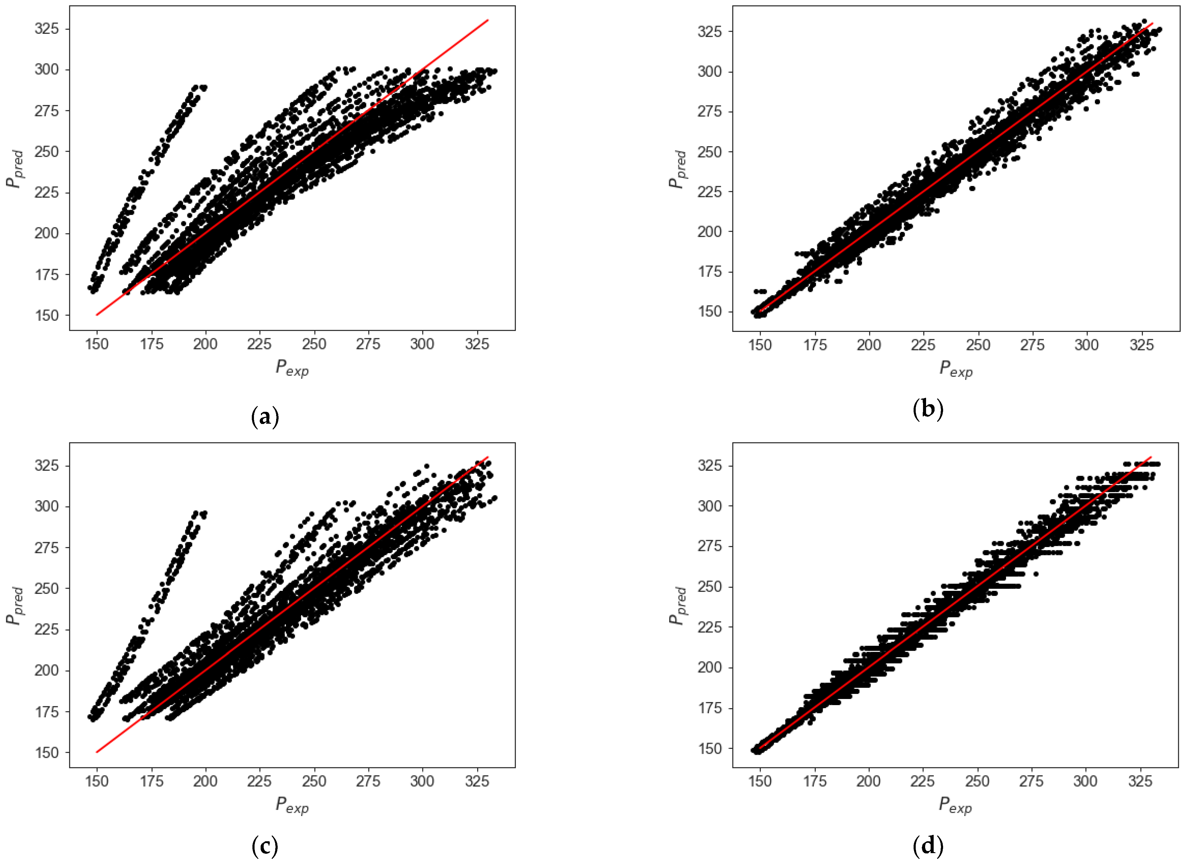
reports the coefficient of determination (R²), mean squared error (MSE), and mean absolute error (MAE) for the selected models (best score) for octane/water using the abundant testing dataset obtained in the CREC VL cell. Figure 21 describes a comparison for the pressures measured and the predicted values, showing that the KNN model provides the best approximation, with an R² value of 0.99 and MSE values as low as 43.78 and 4.91 parameters. The KNN method is selected as the best model to predict the pressure of water/n-octane mixtures in the range of interest.

The best ML model to describe the behavior of pressure for n-octane/water blends is KNN, with this model overcoming the issues of the traditional thermodynamic models involving the Rachford–Rice equations, significantly reducing the uncertainty of any theoretically thermodynamically based algorithm.

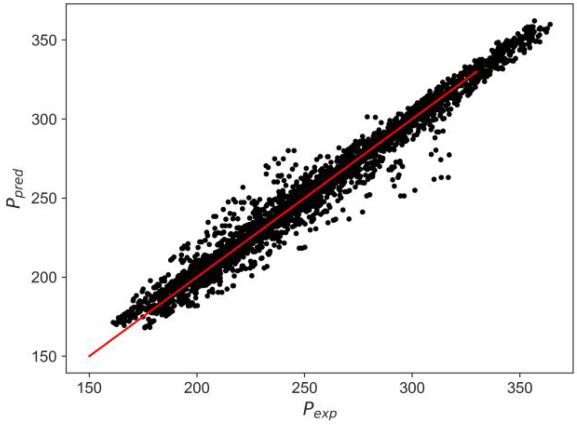
In the same way, if a pseudo-binary mixture is assumed for PASN/water mixtures, a KNN model based on the experimental results can also be applied with an R² = 0.9933 MSE = 34.24 and MAE = 4.41, as presented in Figure 22. The pseudo-component for the PASN is defined using the hydrocarbon blends reported in Table 6.

Although the ML model developed in the present study has the ability to predict vapor pressure efficiently, it requires a significant number of experimental data points allowing for both the training of the proposed model, as well as its validation. In this respect, the availability of laboratory equipment, such as the CREC VL-Cell, providing abundant phase equilibrium data, is critical for both ML model development and validation.

5. Conclusions

(a)

Flash calculations for n-octane/water and PASN/water systems can be described, in principle, using the SRKKD EoS and Rachford–Rice equations. However, the SRKKD EoS and Rachford–Rice equations involve convergence issues in the case of n-octane/water mixtures. These convergence issues were clarified considering the parallelism of the RR_x and RR_y (Rachford–Rice) planes for n-octane/water systems.

(b)

Flash calculations for synthetic naphtha/water (PASN/water) blends implemented using a Python-based algorithm showed numerical solutions free of converging issues, although with numerical solutions showing a lack of accurate prediction of naphtha–water solubility.

(c)

Data from the CREC VL-Cell can be used to propose correlations for the calculation of solubility of n-octane in water and water in n-octane, as well as the equilibrium constant values.

(d)

Data from the CREC VL-Cell and the developed ML approach with the KNN model showed the best performance with, an R² = 0.9911, for accurately predicting the total pressure in water/n-octane mixtures, and R² = 0.9933 in the case of PASN/water mixtures.