Research and Application of Power Grid Maintenance Scheduling Strategy under the Interactive Mode of New Energy and Electrolytic Aluminum Load

Abstract

Formulating a reasonable and feasible unit maintenance scheme is a promising way to eliminate potential risks and improve the reliability of power systems. However, the uncertainty and volatility of new energy outputs, such as wind power, increase the difficulty of scheme formulation. To overcome the complexity of uncertainty, a robust unit maintenance scheme considering the uncertainty of new energy output and electrolytic aluminum load is established in this paper. Considering the significant time-series characteristics of new energy, this paper first introduces the definition and mathematical model of information granulation (IG), through which the initial new energy output data can be transformed into fuzzy particles used for prediction and analysis. Moreover, a support-vector machine (SVM) regression prediction model is adopted, and a corresponding progressive search algorithm is designed to determine SVM parameters efficiently. Then, a robust unit maintenance model is established considering the upper and lower predicted error. In addition, electrolytic aluminum loads are allowed to participate in power system dispatch. Finally, the modified reliability test system–Grid Modernization Lab Consortium (RTS–GMLC test system) and an actual power grid in Southwest China are used to verify the accuracy and feasibility of the proposed method.

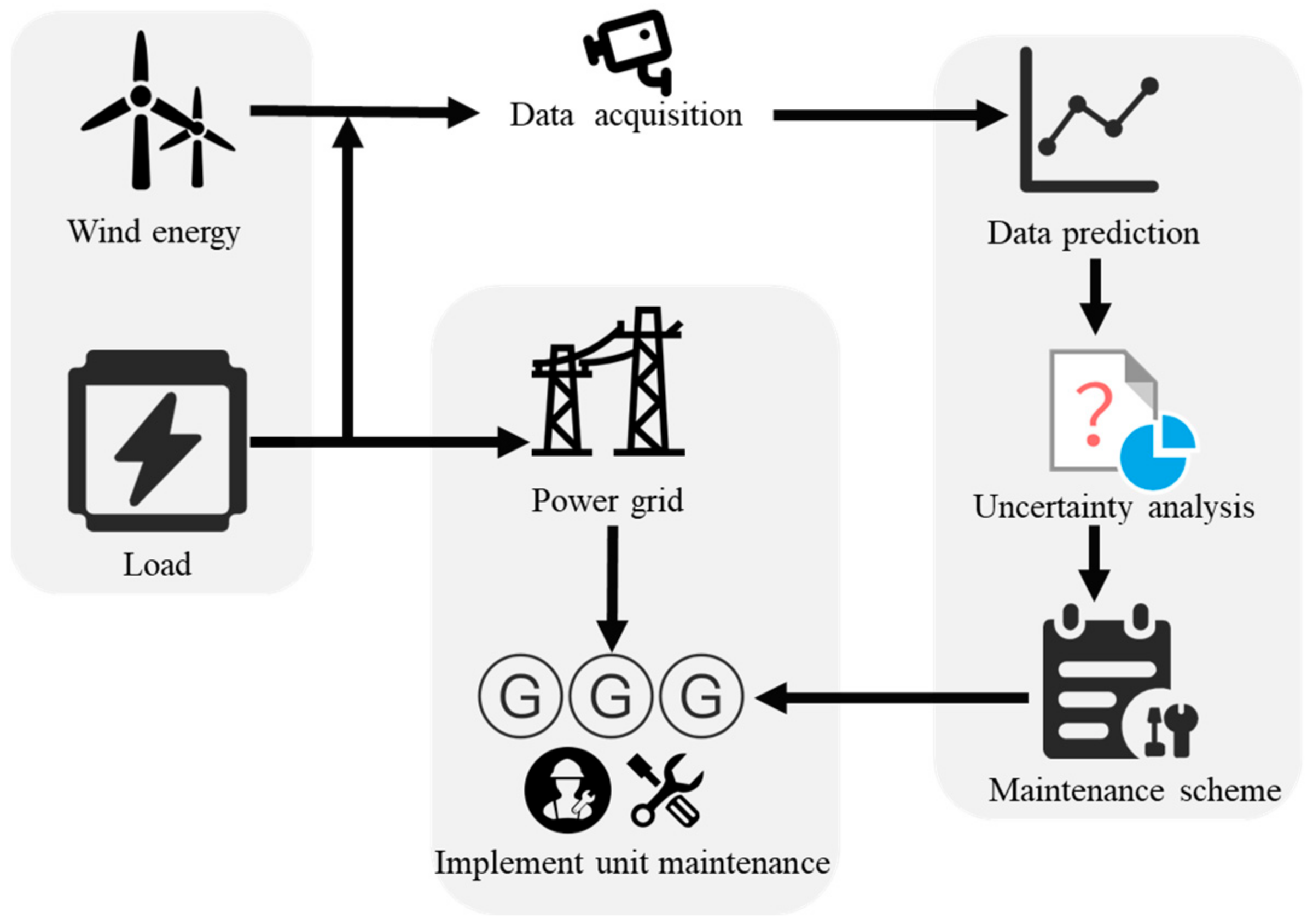
1. Introduction

With the development of the economy and society, load and power generation capacity are growing rapidly. The proportion of new energy is increasing. As mentioned in China’s new energy power generation analysis report, by 2020, the installed capacity of new energy power generation will reach 410 million KW, accounting for 20.6% of the total installed capacity of the country. On the other hand, we can anticipate that with the national goal of “reaching the peak of carbon” and “carbon neutralization”, new energy generation and supporting projects will be developed on a larger scale all over the country in the future. Compared with the traditional thermal power units, although the new energy has the advantages of being clean and sustainable, the fluctuation of its output increases the adverse impact of power systems’ steady-state operation and economic dispatch. Many scholars have carried out valuable research. Some dispatch margin is reserved in [1], considering increased wind generation, which can guarantee the security operation of the power system. To deal with the uncertainty brought by new energy, the authors of [2,3,4] adopted chance constraint, confidence intervals, and fuzzy methods, respectively, and achieved good performance.

The determination of maintenance schemes is an important way to eliminate operational risks and improve the reliability of power systems. Therefore, in the operation scheduling of power systems, the operators must pay attention in order to formulate feasible unit maintenance schemes [5]. At present, the number of units in the system is large, and there are many kinds of units, so more conditions and constraints need to be considered, significantly increasing the complexity of scheme formulation. In addition, maintenance schemes will affect many aspects of power systems, such as reliability assessment and economic dispatch. When the units are scheduled for maintenance, the system output will be reduced, which may bring the risk that the system power supply cannot meet the demand—especially for areas with insufficient power when power consumption peaks. Considering the adverse maintenance effects, preventive maintenance decisions are made via multistage manufacturing systems in [6], some intelligent control methods and management modes are proposed for hydroelectric-generating units and thermal-generating units in [7,8,9] and, for storage systems, a novel maintenance optimization model is built to carry out reliability assessment via sequential inspection in [10].

Above all, unit maintenance decision making is the most critical problem in the power system. At present, a shortage of coal resources sweeping across large swathes of China has forced power rationing in some provinces. A suitable maintenance scheme could bring great benefits and improve equipment efficiency. With the development of the power grid, equipment maintenance decision making has roughly experienced three stages: post-maintenance [11], planned maintenance [12], and condition-based maintenance [13]. If the unit maintenance scheme is not properly arranged, it will not only cause the consumption of power, but also affect the safe and reliable operation of the power system. For this reason, the relevant literature has adopted data-driven methods, GA intelligent algorithms, etc., which enhance the stability of the system.

On the other hand, power systems are very complex artificial systems, and their daily production scheduling process is based on the prediction of unknown factors, i.e., load and new energy output. Many prediction methods have been used, such as BPNN and other ANN methods. Among them, the SVM (support-vector machine) method has good generalization ability, so it is widely used in the field of data prediction [14,15]. SVM was first proposed by Dr. Vapnik. Similar to multilayer perceptron networks and radial basis function networks, SVM can be used in pattern classification and nonlinear regression [16,17]. The main principle of SVM is to establish a classification hyperplane as the decision surface to maximize the isolation edge between positive and negative examples. The generalization error rate of the learning machine is bounded by the sum of the training error rate and a term dependent on the Vapnik–Chervonenkis dimension. In the case of separable modes, the value for the former term is zero, and the latter term is minimized [18].

However, due to the existence of objective conditions such as load forecasting error and random outage of generating units, there are a series of uncertain factors in the operation process of power systems, which are particularly prominent after the large-scale wind power grid is connected. In the actual production scheduling process of power systems, a certain rotating reserve capacity is maintained to deal with the uncertain factors. Once the load or wind power output is inconsistent with the predicted value, the unit undertaking the task of rotating reserve in the system will adjust the output, so as to ensure the power supply of the system. The above method tends to ignore the sequential characteristics of new energy output/load, and cannot fully explore the potential value behind the data, making it difficult to obtain satisfactory results.

Thus, an improved support-vector machine (SVM) regression prediction model based on the information granulation method is proposed in this paper, and can make full use of the sequential characteristics of wind power output. Then, the prediction error is chosen to describe uncertainty, and a corresponding robust unit maintenance model is established.

Figure 1 shows the whole process of drawing up the unit maintenance scheme. The main structure of this paper is as follows: In Section 2, the concept and principle of the IG method is introduced. Based on Section 2, the improved SVM regression prediction model and detailed mathematical model are described in Section 3. The modified RTS–GMLC test system and actual power grid in Southwest China are used to verify the accuracy and feasibility of the proposed method in Section 4. Section 5 summarizes the whole paper and explores the potential research directions for the future.

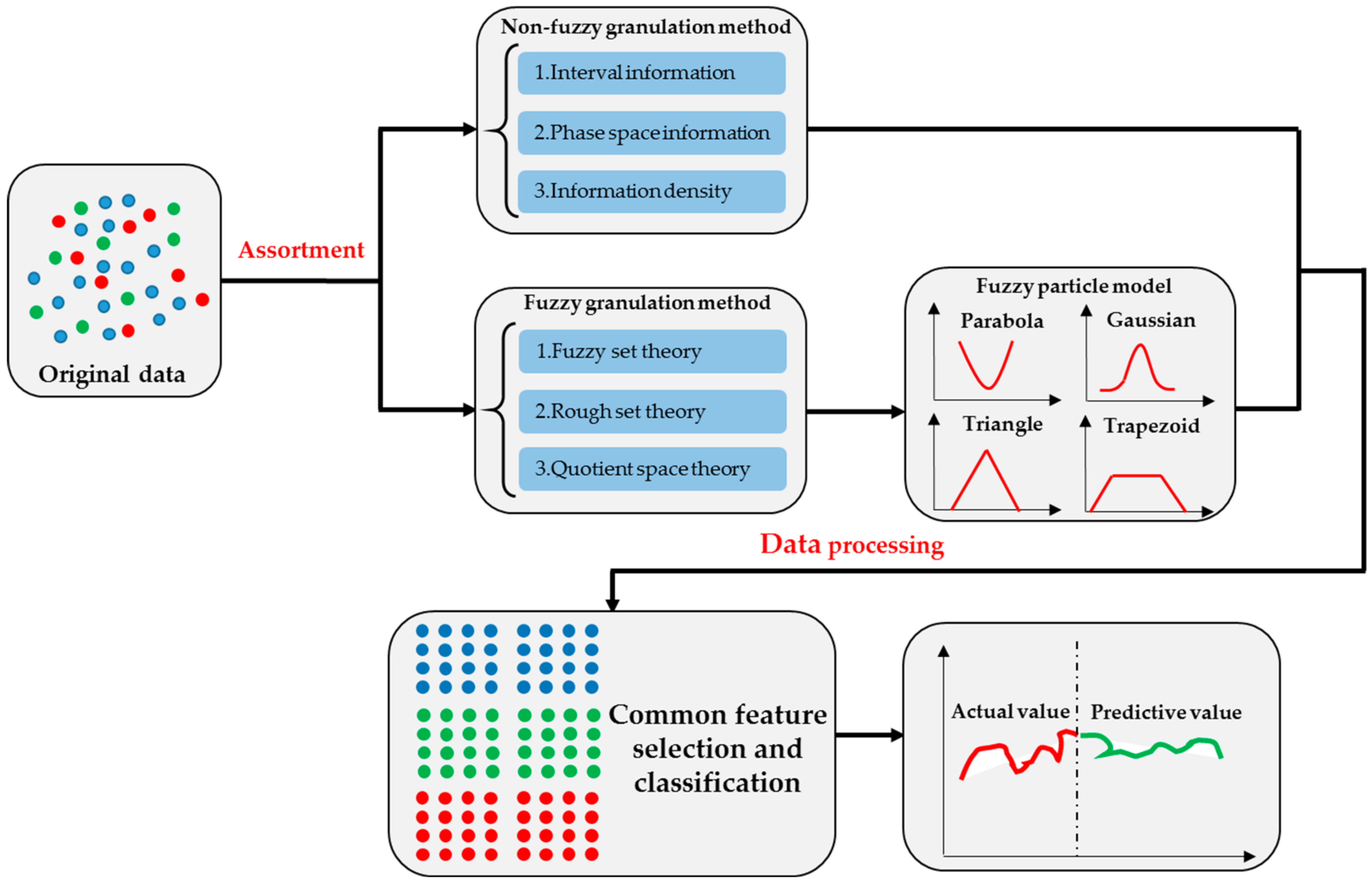
2. Definition and Theory of Information Granulation

The prediction of new energy output is very important for the dispatch and operation of power systems. Traditional prediction methods, such as ANN and least squares methods, tend to ignore the sequential characteristics of data, making it difficult to accurately predict the trend of new energy output and describe uncertainty. In this section, the information granulation (IG) method is introduced to explore the potential behind the data.

The concept of the IG method was first proposed by Professor L. A. Zadeh. Information granulation is used to divide a whole system into several parts for research, and can be seen as a special data clustering method. Each individual part is referred to as an information granule. Generally speaking, an information granule is a set of elements that are combined based on certain data that have similar attributes. Through this method of dealing with data, operators can ignore the unimportant information, and grasp the essential characteristics of the data themselves, thus improving efficiency and simplifying the problem.

As shown in the Figure 2, the IG method can be divided into two types: a non-fuzzy IG method, and a fuzzy IG method. Because most of the attributes of information are fuzzy, the fuzzy IG method is the most commonly used. Information granulation is usually achieved by fuzzy set theory, rough set theory, and quotient space theory. The core of information granulation is to determine a fuzzy particle model. Commonly used fuzzy particle models include parabola, Gaussian, triangular, and trapezoid mathematical models. The corresponding mathematical expressions are shown as (1)–(4), respectively:

$$A(x,a,b,c)=a{x}^2+bx+c,a\ne 0$$

(1)

$$A(x,a,b,c)=a{e}^{-\frac{-{(x-b)}^2}{2c^2}},a>0$$

(2)

$$A(x,a,b,c)=\left\{\begin{array}{ll}0\hfill & x<a\hfill \\ \frac{x-a}{b-a}\hfill & a\le x\le b\hfill \\ \frac{-x+c}{c-b}\hfill & b<x\le c\hfill \\ 0\hfill & x>c\hfill \end{array}\right.$$

(3)

$$A(x,a,b,c,d,k)=\left\{\begin{array}{ll}0\hfill & x<a\hfill \\ \frac{x-a}{b-a}\hfill & a\le x\le b\hfill \\ k\hfill & b<x\le c\hfill \\ \frac{-x+d}{-c+d}\hfill & c<x\le d\hfill \\ 0\hfill & d<x\hfill \end{array}\right.$$

(4)

This paper mainly uses fuzzy set theory to establish the IG model, and the fuzzy particle selects the triangular model. The fuzzy information granulation of new energy output data mainly includes two steps: time window division, and fuzzy processing. Time window division divides the high-dimensional time series into several subsequences in the operation window. The object of fuzzy processing is to generate a time window, and then create fuzzy information particles one by one.

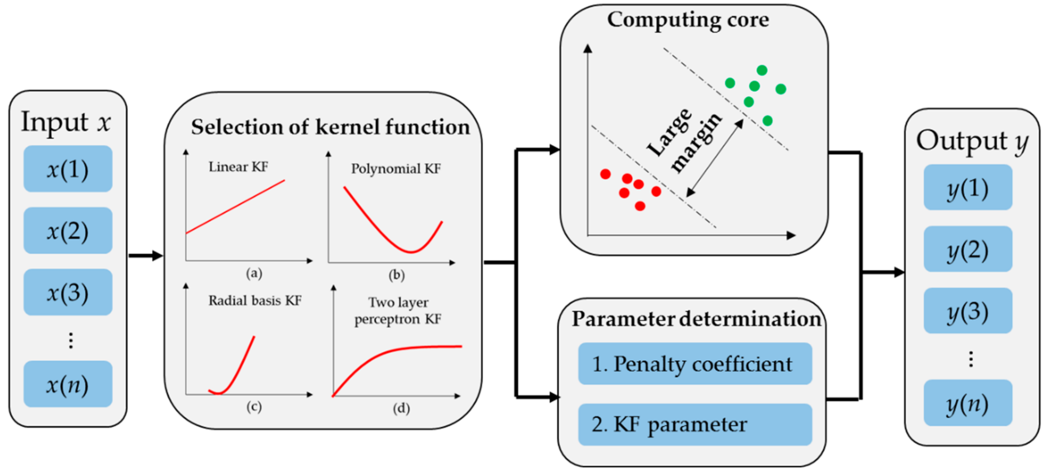
3. Support-Vector Machine Regression Prediction Model

SVM can approach the nonlinear function with the required accuracy to obtain the global optimal solution, and its convergence speed is rapid compared with the traditional ANN algorithm. On the other hand, SVM is outstanding in small training samples, as well as nonlinear and high-dimensional pattern recognition, so it is widely used in regression prediction of time-series data. In this section, the mathematical model of SVM is first introduced in Section 3.1. Then, the progressive search algorithm designed to determine the optimal parameters is shown in Section 3.2.

3.1. Mathematical Model of SVM

The basic principle of SVM is to find the optimal hard margin separating hyperplane in a linearly separable condition and make it meet the following Equation (5):

$$w^{T}x+b=0$$

(5)

where x represents the input vector—i.e., the output data of new energy after information granulation—w is the weight coefficient, and b is the bias. For linearly inseparable cases, the solution of SVM is to map linear inseparable input data into a high-dimensional linear separable feature space via a nonlinear mapping technique (kernel dot product), and classification or regression is done in the feature space. It should be noted that certain points are allowed to dissociate—i.e., introduce relaxation variables to construct a soft margin separation hyperplane, which can be described by the following Equation (6):

$$\begin{array}{c}{\min }_{r,w,b}\frac{1}{2}{‖w‖}^2+C{\displaystyle \sum _{i=1}^m{\xi }_i}\\ \begin{array}{cc}s.t.& y^{(i)}(w^T\phi (x^{(i)})+b)\ge 1-{\xi }_i\end{array}\\ {\xi }_i\ge 0,i=1,\dots ,m\end{array}$$

(6)

where C represents the penalty coefficient, $\phi (x^{(i)})$ represents the mapping function in high-dimensional feature space, and ${\xi }_i$ represents the relaxation variable. Obviously, the model in Equation (6) is a quadratic convex optimization problem, and the Lagrange function is constructed as Equation (7).

$$\begin{array}{l}L(w,b,\xi ,a,r)=\frac{1}{2}{w}^{T}w+C{\displaystyle \sum _{i=1}^m{\xi }_i}-\\ {\displaystyle \sum _{i=1}^m{a}_i\left[y^{(i)}(x^T+b)-1+{\xi }_i\right]}-{\displaystyle \sum _{i=1}^m{\gamma }_i{\xi }_i}\end{array}$$

(7)

Then, the above Lagrange function (7) is substituted into Equation (6), and the dual-optimization mathematical model is obtained as follows:

$$\begin{array}{l}{\max }_{a}W(a)={\displaystyle \sum _{i=1}^m{a}_i-\frac{1}{2}}{\displaystyle \sum _{i,j=1}^m{x}^{(i)}}{y}^{(i)}{a}_i{a}_j〈\varphi (x^{(i)}),\varphi (x^{(j)})〉\\ \begin{array}{cc}s.t.& 0\le a_i\le C,i=1,\dots ,m\end{array},{\displaystyle \sum _{i=1}^m{a}_i}{y}^{(i)}=0\end{array}$$

(8)

The mathematical meaning of the model in (8) is to find the separation hyperplane with the maximum spatial margin. Therefore, the regression function of the SVM can be obtained as Equation (9):

$$f(x)={\displaystyle \sum _{i=1}^n{a}_i}{y}^{(i)}〈\varphi (x^{(i)}),\varphi (x^{(j)})〉+b$$

(9)

The mathematical model of regression function is simplified with the help of the inner product kernel defined by Mercer’s theorem:

$$K(x^{(i)},x^{(j)})=〈\varphi (x^{(i)}),\varphi (x^{(j)})〉$$

(10)

Then, (10) is substituted into (9), and Equation (11) can be obtained as follows:

$$f(x)={\displaystyle \sum _{i=1}^n{a}_i}{y}^{i}K(x^{(i)},x^{(j)})+b$$

(11)

Finally, the regression prediction value of input data x can be calculated by Equation (11).

In order to more intuitively verify the performance of the SVM, this paper uses the mean square error (MSE) and squared correlation coefficient (r²) as the assessment indices. The corresponding mathematical calculation formula is as follows:

$$MSE=\frac{1}{n}{\displaystyle \sum _{i=1}^n{(f(x_i)-y_i)}^2}$$

(12)

$$r^2=\frac{{(n{\displaystyle \sum _{i=1}^{n}f(x_i)}{y}_i-{\displaystyle \sum _{i=1}^{n}f(x_i){\displaystyle \sum _{i=1}^n{y}_i}})}^2}{(n{\displaystyle \sum _{i=1}^{n}f{(x_i)}^2-}({\displaystyle \sum _{i=1}^{n}f(x_i){)}^2})(n{\displaystyle \sum _{i=1}^n{(y_i)}^2-}({\displaystyle \sum _{i=1}^n(y_i){)}^2})}$$

(13)

where n represents the number of samples, x_i represents the ith input datum, f(x_i) represents the ith training output datum, and y_i represents the actual data.

To gain a better understanding, Figure 3 is given to show the whole data processing flow. There are four common kernel functions (KFs), including linear, polynomial, radial basis, and two-layer perception KFs. The core of SVM calculation is to find the separation hyperplane with the maximum margin in high-dimensional feature space. The parameters that need to be determined mainly include the penalty coefficient C and kernel function parameter G. How to efficiently determine these two parameters is still a challenge. Thus, a novel progressive search algorithm was designed to solve this problem, and the detailed steps are discussed in the next section.

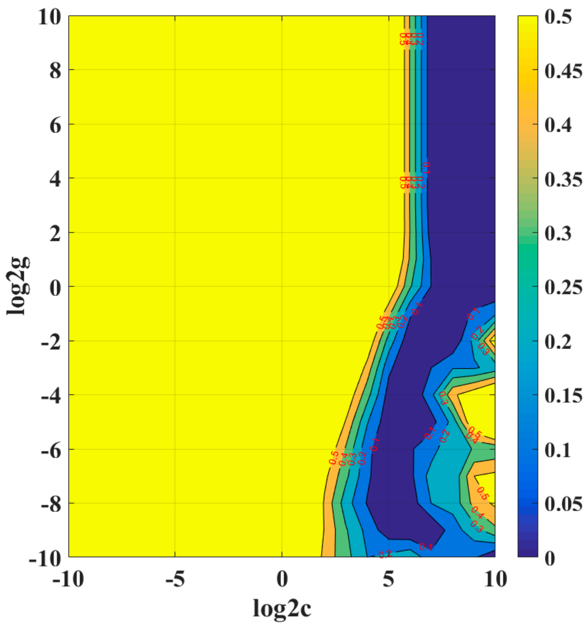
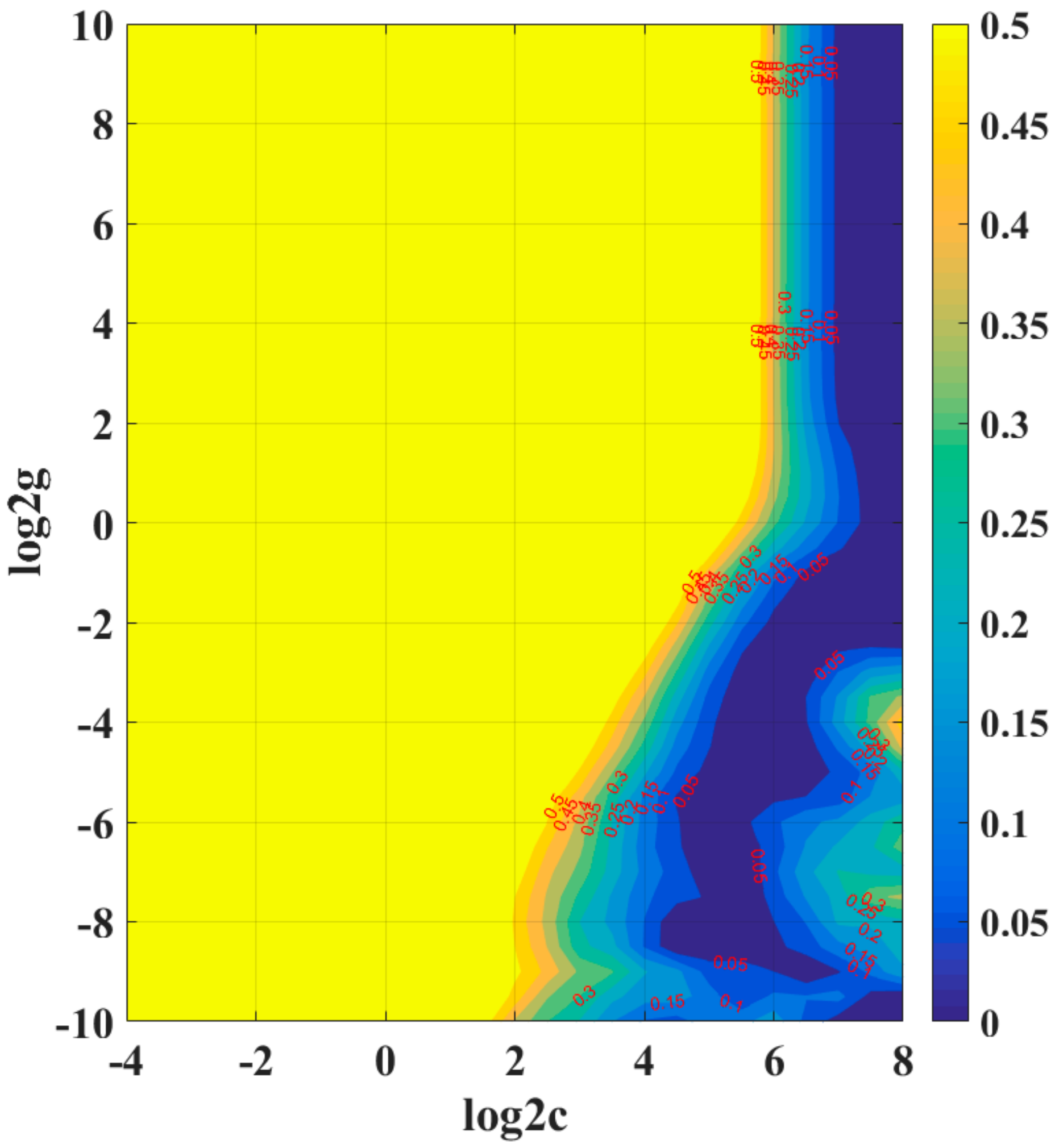
3.2. Progressive Search Algorithm

In previous studies, the penalty parameter C and kernel function (KF) parameter G were arbitrarily given or determined by experience, making it difficult to meet the requirement of high precision. The idea of a cross-validation (CV) method can achieve the optimal parameter value in the majority of cases, effectively avoiding the occurrence of over-learning or under-learning, and finally getting an ideal accuracy for the prediction of the test set. In this paper, the K-fold cross-validation (K-CV) method is adopted, and its detailed steps are as follows:

Firstly, divide the original data into k groups evenly, make a verification set for each data subset separately, and then use the rest of the k−1 subset data as the training set. In this way, k different models will be obtained. The average of the regression prediction accuracy of the k verification sets will be used as the performance index with the K-CV method. The value of k is generally larger than or equal to 2 theoretically. In actual operation, it is generally taken from 3; only when the amount of data in the original dataset is small will it try to take 2. Compared with other methods, such as the hold-out method and leave-one-Out cross-validation (LOO-CV), the K-CV method can effectively avoid the occurrence of over-learning and under-learning; thus, its final results are persuasive.

In addition, different combinations of C and G may achieve the same regression prediction effect. In this situation, select the group with the smallest value of parameter C for the optimal parameters to achieve the highest regression prediction accuracy. If there are multiple groups corresponding to the smallest value of parameter C, then select the first group’s C and G as the optimal parameters. The reason for this is that too large a value of the penalty parameter C will lead to the occurrence of over-learning, i.e., the regression prediction accuracy of the training set is very high and the regression prediction accuracy of the test set is very low (the generalization ability of the regression prediction is reduced). Therefore, in all combinations of penalty parameter C and kernel function (KF) parameter G that can achieve the highest accuracy, it is considered that the smaller value of penalty parameter C is the better selection object.

At the same time, in order to improve the computational efficiency, the values of C and G are discretized with a base-2 logarithm and searched gradually—that is, firstly, the values of C and G can be changed with a large step to roughly determine the range of parameters to be calculated; then, a small-step search is used to accurately determine the parameter value.

4. Designation of a Robust Unit Maintenance Scheme

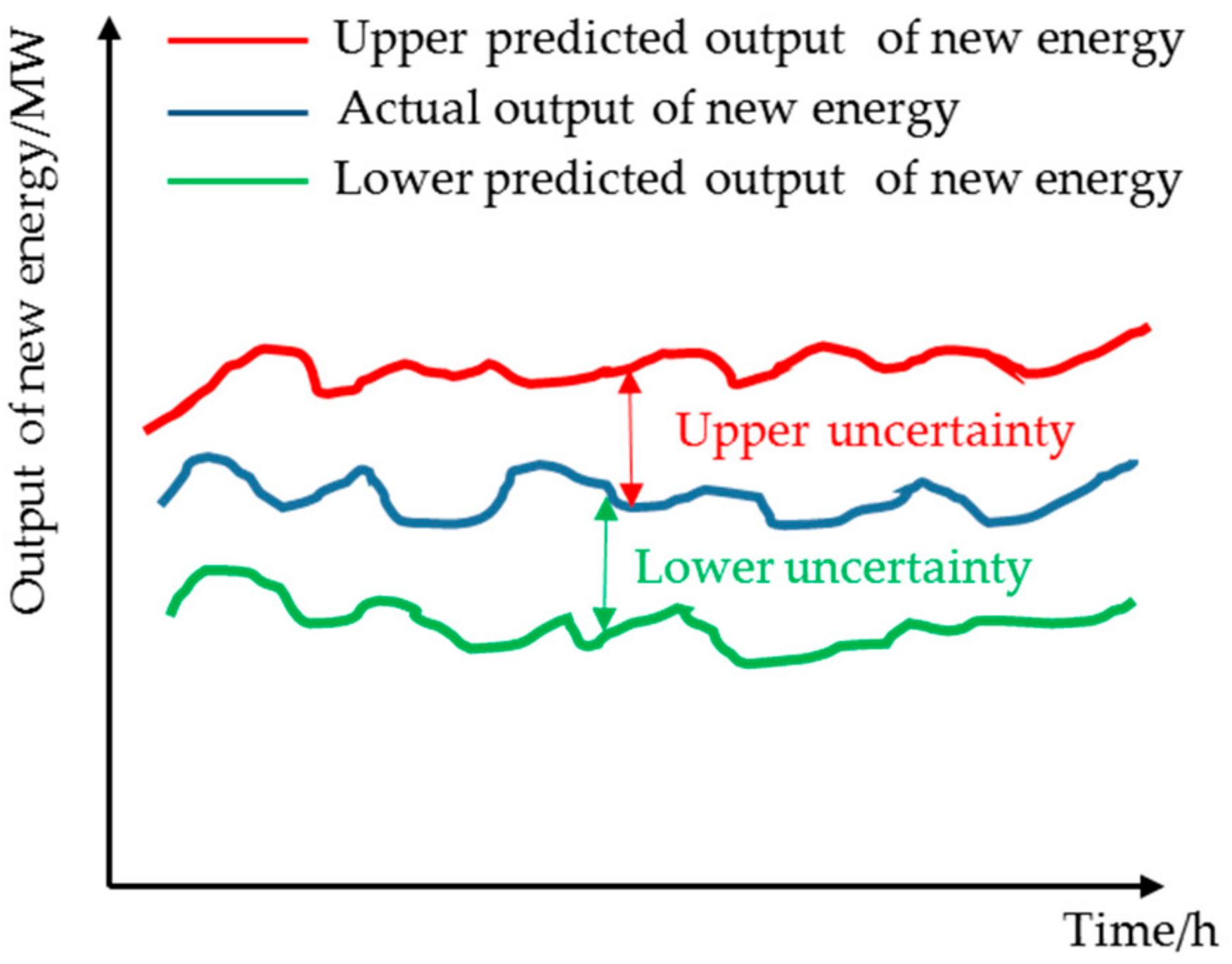
4.1. Analysis of Uncertainty

The traditional uncertain modeling method is used to give an uncertain interval; however, some challenges remain. If the range of the uncertain interval is too small, it will lead to insufficient system safety margins and increased operational risk. On the other hand, if the range is too large, the calculation results will be conservative and unable to make full use of new energy, resulting in weak consumption capacity of new energy and economic losses. Therefore, it is very important to give a reasonable and reliable prediction uncertainty interval. Combined with the above, this paper uses the information granulation method to extract the upper value, lower value, and average value of wind farm output in time series. The uncertainty analysis is carried out to obtain the upper uncertainty and lower uncertainty of new energy output prediction, as shown in the Figure 4, so as to realize the accurate modeling of new energy output uncertainty.

4.2. Mathematical Model of Robust Unit Maintenance

New energy, including wind and hydro resources, is mainly concentrated in the northwest and southwest regions of China. In addition to the common load, these regions also include a certain proportion of electrolytic aluminum load. Therefore, the characteristics of electrolytic aluminum load need to be taken into account when formulating the maintenance plan. The robust unit maintenance model considering the output uncertainty of new energy and electrolytic aluminum load can be expressed by the following mathematical model:

$$\begin{array}{cc}obj:& \end{array}{\displaystyle \sum _{i=1}^k{\lambda }_W(P_{w,t}^{pre,i}-P_{w,t}^{real,i})}+{\displaystyle \sum _{t=1}^T{\lambda }_L(P_{eie,t}-P_{eie,t}^{ori})+}{F}_{coal,u}$$

(14)

$$\mathrm{Here} F_{coal,i,t}=u_{d,i,t}(b_{un,i}-b_{r,\min ,i}){\delta }_i{P}_{G,t}^i{C}_{coal}$$

(15)

$$\begin{array}{cc}s.t.& f(v_i,{\theta }_i,P_i,Q_i)=0\end{array}$$

(16)

$${\varphi }_t^i{P}_{G,t}^{i,\min }\le {\varphi }_t^i{P}_{G,t}^i\le {\varphi }_t^i{P}_{G,t}^{i,\max }$$

(17)

$$P_l^{\min }\le P_{l,t}\le P_l^{\max }$$

(18)

$${\displaystyle \sum _{i=1}^N{\varphi }_t^i{P}_{G,t}^i}+{\displaystyle \sum _{i=1}^k{P}_{w,t}^{real,i}}\ge {\displaystyle \sum _{i=1}^m{P}_{load,t}^i}+P_{eie,t}^{}+R_r$$

(19)

$$t_{off}^i\ge t_{down}^i,t_{on}^i\ge t_{up}^i$$

(20)

$$P_{w,t}^{real,i}+{\mu }_t^i\le P_{w,t}^{\max ,i}$$

(21)

$${\mu }_t^{i,\min }\le {\mu }_t^i\le {\mu }_t^{i,\max }$$

(22)

$$-R_{down}\le {\varphi }_t^i{P}_{G,t}^i-{\varphi }_{t-1}^i{P}_{G,t-1}^i\le R_{up}$$

(23)

$${\displaystyle \sum _{t=1}^T(\alpha P_{eie,t}^{ori}+\beta (P_{eie,t}^{ori}-P_{eie,\min }))}=Y^{order}$$

(24)

$$h=\left\{\begin{array}{cc}1& {\varphi }_t^i=1,{\varphi }_{t-1}^i=0\\ 0& else\end{array}\right.$$

(25)

$${\tau }_t^i=\{\begin{array}{l}1,\begin{array}{cc}when& t\notin [t_{m-s}^i,t_{m-e}^i]\end{array}\hfill \\ 0,else\end{array}$$

(26)

$${\displaystyle \sum _{i=1}^N{\tau }_t^i}=N{T}_{dis}-{\displaystyle \sum _{i=1}^N{T}_{dur}^i}$$

(27)

$${\displaystyle \sum _{t=t_{m-s}}^{t_{m-e}}{\tau }_t^i\le 1}$$

(28)

$$P_{G,t}^i=0,\begin{array}{cc}when& t\in [t_{m-s}^i,t_{m-e}^i]\end{array}$$

(29)

$$\frac{P_{eie,t}}{P_{eie,t}+{\displaystyle \sum _{i=1}^m{P}_{load,t}^i}}\le 0.06$$

(30)

Here, the objective function (14) refers to the minimum sum of the wind abandonment penalty cost, the power regulation cost of electrolytic aluminum load, and the deep peak shaving cost of thermal power units. The detailed calculation method of the deep peak shaving cost of thermal power units is shown in Equation (15). Equation (16) represents the power flow equation constraint. Equation (17) represents the generator output constraint. Equation (18) represents the line active power constraint to avoid overload of transmission lines. Equation (19) represents the power balance constraint. Equation (20) represents the unit startup and shutdown time constraint. Equation (21) represents the wind power output constraint. Equation (22) represents the uncertainty constraint of wind power prediction output. It should be noted that the upper and lower limits of uncertainty here are obtained through the improved SVM model based on the IG method mentioned above. Equation (23) represents the unit ramp rate constraint. Equation (24) represents the relationship between power and yield before electrolytic aluminum load participating in demand response. Equation (25) represents the calculation equation of the unit startup and shutdown state coefficient. Equation (26) represents the maintenance time window constraint, i.e., the maintenance is only scheduled at a specific time. Equation (27) represents the total maintenance time constraint. Equation (28) represents the maintenance continuity constraint. Equation (29) represents the unit output constraint during maintenance. Equation (30) represents the allowable power regulation range of the electrolytic aluminum load. In this paper, the penalty coefficient of wind abandonment ${\lambda }_w$ is 1000 and the reward coefficient of load regulation in the electrolytic aluminum load ${\lambda }_L$ is 800. The detailed description of other variables is shown in Nomenclature.

There is one point needed to explain the optimization model proposed in this paper: when the power consumption of the electrolytic aluminum load changes, the total load of the system will also change. As shown in Equation (30), at time t, when the power consumed by the electrolytic aluminum load decreases, the proportion of electrolytic aluminum load in the total load will also decrease. In order to better judge the power variation range of the electrolytic aluminum load, Figure 5 is given to judge the power regulation range of the electrolytic aluminum load.

5. Results Analysis

In this section, the feasibility and accuracy of the proposed method can be observed in several cases.

5.1. Case Study 1: RTS–GMLC Test System

5.1.1. The Result of the IG Method

The wind power data used in this paper are from a wind farm in a certain area of the United States, with longitude of −93.433685 and latitude of 40.877926. The value of wind power was measured each hour. This paper selects a total of 2260 points from 6500 to 8760 for information granulation, as shown in Figure 6.

The result of information granulation is shown in Figure 7. After granulation processing, the initial wind power information is decomposed into three data dimensions, namely, the average value, upper value, and lower value. Among them, the blue point represents the lower value after information granulation, the green point represents the upper value after information granulation, and the red point represents the average value after information granulation.

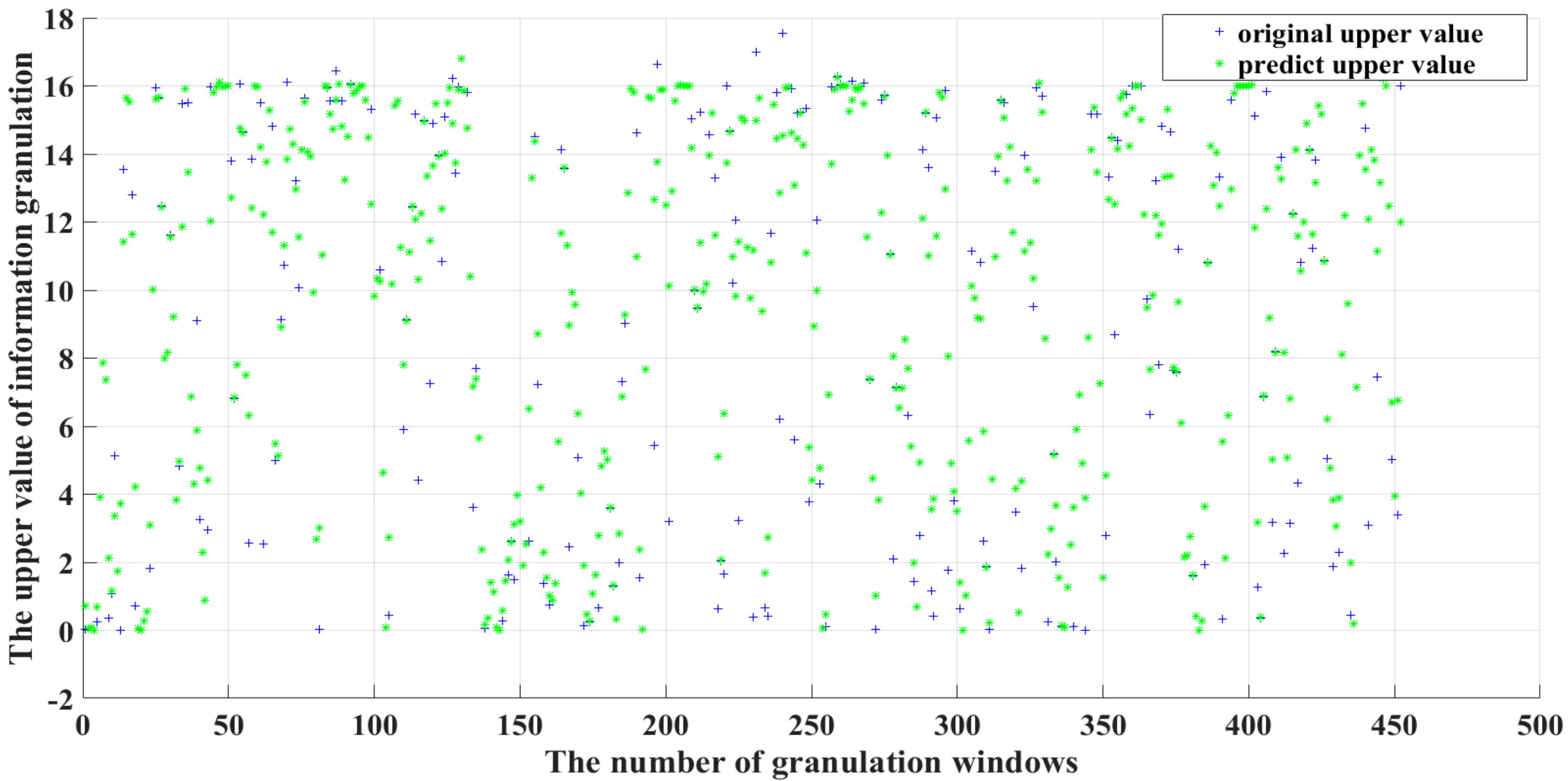
5.1.2. The Result of the SVM Model

The wind power data processed by information granulation—including the information on the average value, upper value, and lower value—were respectively input as the training data of the SVM. Through the progressive search algorithm, the optimal value of penalty coefficient C and kernel function (KF) parameter G were finally determined. The numerical simulation was carried out using MATLAB R2016b on a personal laptop with Windows 7, 16 GB of memory, and an i5-7300HQ processor.

The calculation results are shown in Figure 8, Figure 9, Figure 10 and Figure 11. In Figure 9 and Figure 11, different colors represent the mean square error (MSE), which can be calculated by Equation (13), and several advantages can be observed and summed up.

1. Prediction accuracy of the SVM model: It can be seen from Figure 8 and Figure 10 that the coincidence between input data points and output data points is very high. The prediction error of the upper data is 3.2%, and the prediction error of the lower data is 2.7%. This shows the high accuracy of the SVC model in data prediction, which can effectively describe the change trend of new energy output, and then reduce the conservatism of traditional robust methods;

2. Feasibility of the progressive search algorithm: As shown in Figure 9 and Figure 11, the progressive search algorithm first roughly determines the penalty coefficient C and the kernel function parameter G, and then carries out a fast search in the yellow area in the figure—that is, the area with large MSE—to reduce the computing time. In the blue area with small value of MSE, the algorithm adopts a small step for analysis and calculation. The total calculation time is 89.976 s. Considering that the time scale of China’s power grid dispatching is 5–15 min, the proposed method meets the needs of online calculation of the actual power grid system.

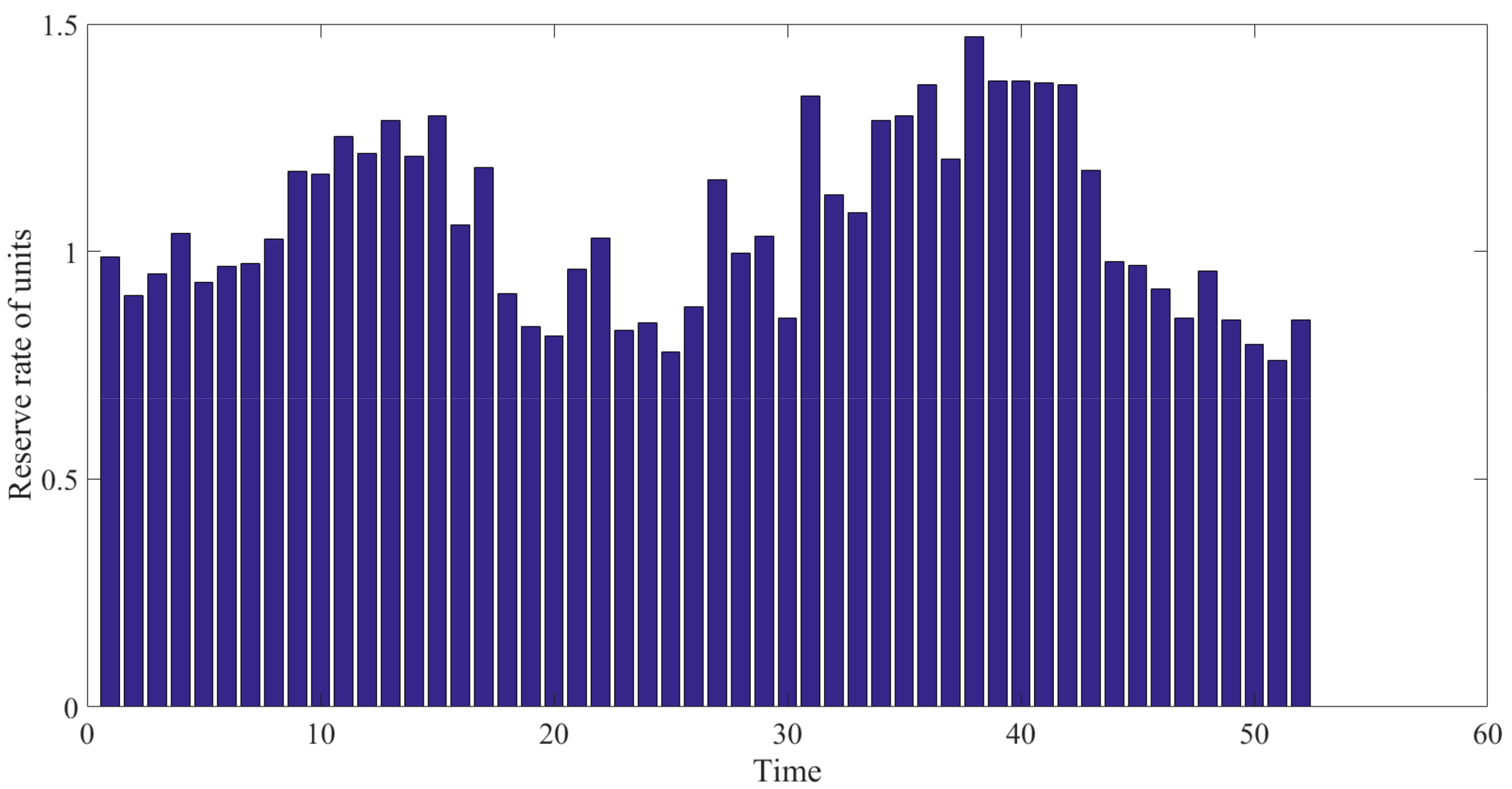
5.1.3. The Result of the Robust Unit Maintenance Model

In this paper, the modified RTS–GMLC test system was used to verify the feasibility of the maintenance model. Here, two wind farms were connected at nodes 5 and 11, and an energy-intensive enterprise was located at node 17. The total operation time scale was 52 h. The optimal maintenance scheme was calculated using Equations (14)–(30), and the solver adopted was Gurobi. The total solution time was 47.0623 s, and the optimal total cost obtained by the model was USD 12,756.0. The maintenance schedule of each unit is as follows (

Table 1. The maintenance schedule of each unit in the RTS–GMLC test system.

Unit Number	Downtime Period Available for Maintenance	Unit Number	Downtime Period Available for Maintenance
1	4–7	11	2–5
2	5–6	12	8–13
3	20–22	13	9–11
4	31–34	14	42–46
5	23–28	15	28–31
6	11–14	16	12–14
7	21–25	17	25–26
8	44–46	18	26–27
9	19–21	19	11–12
10	17–19	20	37–39

):

At this time, the unit reserve rate of the system is shown in Figure 12.

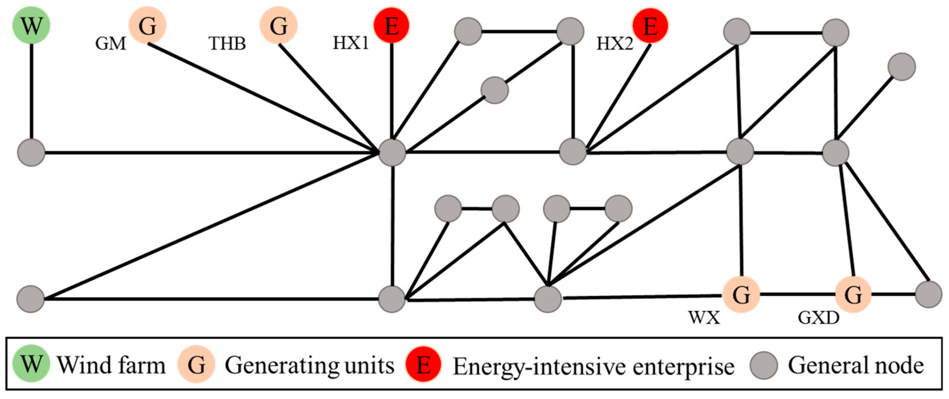
5.2. Case Study 2: Actual Power Grid in Southwest China

An actual power grid in Southwest China was used to further illustrate the accuracy of the proposed method. The regional power grid includes one wind farm, two energy-intensive enterprises—i.e., electrolytic aluminum load—and several substations with different voltage levels. The detailed topology of the actual power grid in Southwest China is shown in Figure 13. There are 20 units in this system, and the total maintenance time is 24 h.

By calculating Equations (14)–(30), the optimal downtime period available for the maintenance of each unit can be obtained. The total calculation time is 36.34 s. The detailed calculation results are shown in

Table 2. The results comparison between different models.

Model	Average Wind Power Curtailment Rate/%	Total Cost/USD
Model proposed in this paper	1.21	52,272
Model not considering electrolytic aluminum load	1.97	85,104

and

Table 3. The maintenance schedule of each unit in the actual power grid in Southwest China.

Unit Number	Downtime Period Available for Maintenance	Unit Number	Downtime Period Available for Maintenance
1	5–7	11	20–22
2	8–11	12	1–3
3	13–15	13	2–5
4	8–9	14	14–17
5	5–6	15	6–8
6	6–8	16	3–5
7	11–13	17	12–14
8	17–19	18	18–20
9	6–7	19	7–9
10	20–23	20	19–22

. Meanwhile, in order to better verify the effectiveness of the proposed method, the following comparison is made in this paper: firstly, the dispatch flexibility provided by the electrolytic aluminum load is ignored, i.e., the power consumed by the electrolytic aluminum load is seen as a constant value. Under these conditions, the average wind power curtailment rate is 1.97%, and the penalty cost caused by wind curtailment is USD 85,104. When incentive policies are adopted to guide the electrolytic aluminum load to participate in dispatching, the average wind power curtailment rate is 1.21%, and the value of objective function is USD 52,272. Obviously, because the reward cost for the participation of the electrolytic aluminum load is lower than the penalty cost for wind curtailment, the total economic investment of the system will also be reduced. In general, the model proposed in this paper has significant advantages in terms of economic and environmental benefits.

6. Conclusions and Future Work

In order to reduce the conservatism of the traditional robust model, this paper first adopted the information granulation method to extract the upper and lower information of wind power output. Then, the SVM model and progressive search algorithm were designed to predict the upper and lower data, respectively, in order to determine the change trend of new energy output accurately, and the robust maintenance model was finally solved through Gurobi. The accuracy and feasibility of the proposed method can be seen from the cases. In future research, some more mature linearization methods and uncertainty modeling methods will be studied to improve the new energy consumption level and economic performance of the system.

In future research, the following can be carried out:

1.

Study the economic dispatching and unit maintenance methods of power systems under the background of low carbon emissions. Traditional thermal power-generating units will produce a lot of carbon dioxide in the process of power generation, but if power grids rely too much on new energy, such as wind power and light energy, it will increase the risk during system operation. How to strike a balance between low-carbon economic production and reliable operation of power systems remains a challenge;

2.

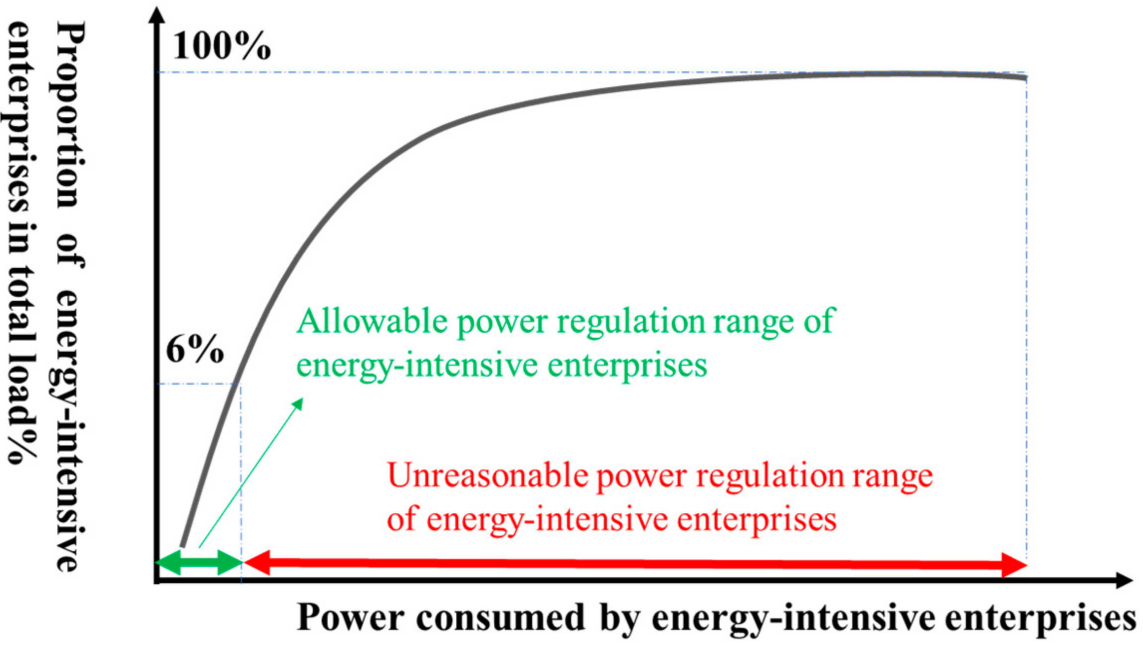
How to formulate a demand response plan during maintenance is also an urgent problem to be solved. During the maintenance period, the output of the unit is reduced sharply. At this time, the power grid can encourage consumers to reduce the demand for load power. On the premise of meeting their basic living requirements, they can achieve a win–win situation for both sides by adjusting the working conditions of air conditioning, lighting, heating equipment, etc.

References

- Hedayati-Mehdiabadi, M.; Zhang, J.; Hedman, K.W. Wind Power Dispatch Margin for Flexible Energy and Reserve Scheduling with Increased Wind Generation. IEEE Trans. Sustain. Energy 2015, 6, 1543–1552. [Google Scholar] [CrossRef]
- Wang, Z.; Shen, C.; Liu, F.; Wu, X.; Liu, C.-C.; Gao, F. Chance-Constrained Economic Dispatch With Non-Gaussian Correlated Wind Power Uncertainty. IEEE Trans. Power Syst. 2017, 32, 4880–4893. [Google Scholar] [CrossRef]
- Li, P.; Yang, M.; Wu, Q. Confidence Interval Based Distributionally Robust Real-Time Economic Dispatch Approach Considering Wind Power Accommodation Risk. IEEE Trans. Sustain. Energy 2021, 12, 58–69. [Google Scholar] [CrossRef]
- Miranda, V.; Hang, P.S. Economic Dispatch Model with Fuzzy Wind Constraints and Attitudes of Dispatchers. IEEE Trans. Power Syst. 2005, 20, 2143–2145. [Google Scholar] [CrossRef] [Green Version]
- Feng, C.; Wang, X. A Competitive Mechanism of Unit Maintenance Scheduling in a Deregulated Environment. IEEE Trans. Power Syst. 2009, 25, 351–359. [Google Scholar] [CrossRef]
- Huang, J.; Chang, Q.; Zou, J.; Arinez, J. A Real-Time Maintenance Policy for Multi-Stage Manufacturing Systems Considering Imperfect Maintenance Effects. IEEE Access 2018, 6, 62174–62183. [Google Scholar] [CrossRef]
- Mirsaeedi, H.; Fereidunian, A.; Mohammadi-Hosseininejad, S.M.; Dehghanian, P.; Lesani, H. Long-Term Maintenance Scheduling and Budgeting in Electricity Distribution Systems Equipped With Automatic Switches. IEEE Trans. Ind. Inform. 2018, 14, 1909–1919. [Google Scholar] [CrossRef]
- Abiri-Jahromi, A.; Fotuhi-Firuzabad, M.; Parvania, M. Optimized Midterm Preventive Maintenance Outage Scheduling of Thermal Generating Units. IEEE Trans. Power Syst. 2012, 27, 1354–1365. [Google Scholar] [CrossRef]
- Fu, C.; Ye, L.; Liu, Y.; Yu, R.; Iung, B.; Cheng, Y.; Zeng, Y. Predictive Maintenance in Intelligent-Control-Maintenance-Management System for Hydroelectric Generating Unit. IEEE Trans. Energy Convers. 2004, 19, 179–186. [Google Scholar] [CrossRef]
- Bai, S.; Cheng, Z.; Guo, B. Maintenance Optimization Model with Sequential Inspection Based on Real-Time Reliability Evaluation for Long-Term Storage Systems. Processes 2019, 7, 481. [Google Scholar] [CrossRef] [Green Version]
- Chen, A.; Blue, J. Recipe-Independent Indicator for Tool Health Diagnosis and Predictive Maintenance. IEEE Trans. Semicond. Manuf. 2009, 22, 522–535. [Google Scholar] [CrossRef]
- Nourelfath, M.; Fitouhi, M.-C.; Machani, M. An Integrated Model for Production and Preventive Maintenance Planning in Multi-State Systems. IEEE Trans. Reliab. 2010, 59, 496–506. [Google Scholar] [CrossRef]
- Chen, H.; Lu, N.; Jiang, B.; Xing, Y. Condition-based maintenance optimization for continuously monitored degrading systems under imperfect maintenance actions. J. Syst. Eng. Electron. 2020, 31, 841–851. [Google Scholar] [CrossRef]
- Zhang, X.; Wang, S.; Zhao, Y. Application of support vector machine and least squares vector machine to freight volume forecast. In Proceedings of the 2011 International Conference on Remote Sensing, Environment and Transportation Engineering, Nanjing, China, 24–26 June 2011; pp. 104–107. [Google Scholar]
- Ertekin, Ş.; Bottou, L.; Giles, C.L. Nonconvex Online Support Vector Machines. IEEE Trans. Pattern Anal. Mach. Intell. 2010, 33, 368–381. [Google Scholar] [CrossRef] [PubMed] [Green Version]
- Mohan, L.; Pant, J.; Suyal, P.; Kumar, A. Support Vector Machine Accuracy Improvement with Classification. In Proceedings of the 2020 12th International Conference on Computational Intelligence and Communication Networks (CICN), Bhimtal, India, 25–26 September 2020; pp. 477–481. [Google Scholar]
- Sun, B.; Song, S.-J.; Wu, C. A new algorithm of support vector machine based on weighted feature. In Proceedings of the 2009 International Conference on Machine Learning and Cybernetics, Baoding, China, 12–15 July 2009; Volume 3, pp. 1616–1620. [Google Scholar]
- Kong, R.; Zhang, B. Autocorrelation Kernel Functions for Support Vector Machines. In Proceedings of the Third International Conference on Natural Computation (ICNC 2007), Haikou, China, 24–27 August 2007; Volume 1, pp. 512–516. [Google Scholar]