Dynamic Modeling of a Nonlinear Two-Wheeled Robot Using Data-Driven Approach

 , , and
Abstract
:1. Introduction
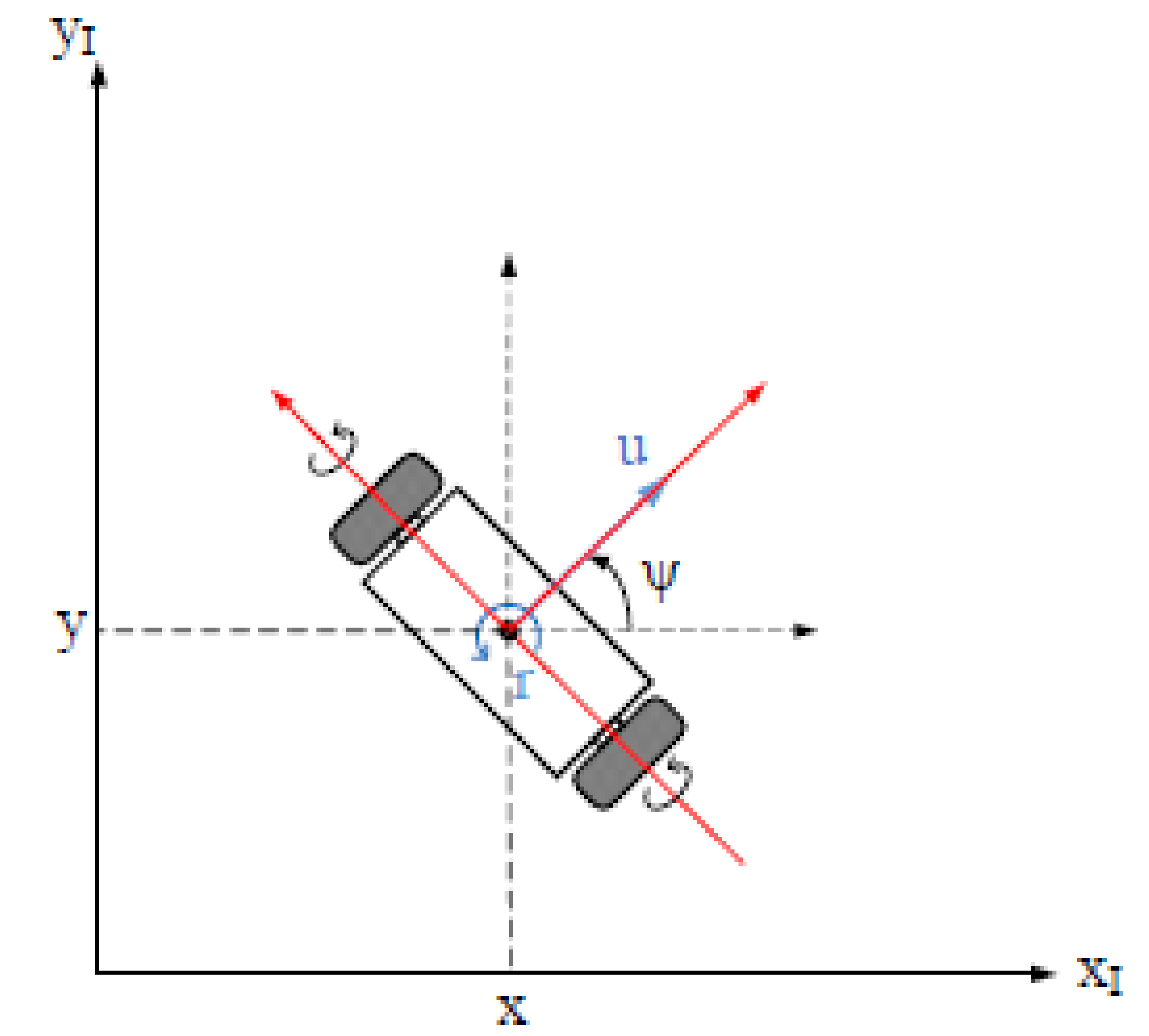
2. TWR Dynamics Moving on a Planar Surface and ARX Model Structure
2.1. ARX Model Structure
2.2. NLARX Model Structure
3. Methodology
4. Simulation and Results
4.1. Dataset Generation
4.2. Estimated Results of the NLARX Model
5. Discussion and Analysis
6. Conclusions
Author Contributions
Funding
Institutional Review Board Statement
Informed Consent Statement
Data Availability Statement
Acknowledgments
Conflicts of Interest
References
- Ljung, L. Perspectives on system identification. Annu. Rev. Control 2010, 34, 1–12. [Google Scholar] [CrossRef] [Green Version]
- Berardi, U. Modelling and testing of a dielectic electro-active polymer (DEAP) actuator for active vibration control. J. Mech. Sci. Technol. 2013, 27, 1–7. [Google Scholar] [CrossRef]
- Kim, Y.; Kim, Y.H.; Lee, S. Multivariable nonlinear identification of smart buildings. Mech. Syst. Signal Process. 2015, 62, 254–271. [Google Scholar] [CrossRef]
- Cheng, T.M.; Savkin, A.V.; Celler, B.G.; Su, S.W.; Wang, L. Nonlinear modeling and control of human heart rate response during exercise with various work load intensities. IEEE Trans. Biomed. Eng. 2008, 55, 2499–2508. [Google Scholar] [CrossRef] [PubMed]
- Kim, Y.; Kim, J.M.; Kim, Y.H. System identification of smart buildings under ambient excitations. J. Meas. 2016, 87, 294–302. [Google Scholar] [CrossRef]
- Peltier, M.D. Trajectory Control of a Two-Wheeled Robot. Master’s Thesis, University of Rhode Island, Kingston, RI, USA, 2012. [Google Scholar]
- Nomura, T.; Kitsuka, Y.; Suemitsu, H.; Matsuo, T. Adaptive backstepping control for a two-wheeled autonomous robot. In Proceedings of the 2009 ICCAS-SICE 2009, Fukuoka, Japan, 18–21 August 2009; pp. 4687–4692. [Google Scholar]
- Chan, R.P.M.; Stol, K.A.; Halkyard, C.R. Review of modelling and control of two-wheeled robots. Annu. Rev. Control 2013, 37, 89–103. [Google Scholar] [CrossRef]
- Uddin, N. Lyapunov-based control system design of two-wheeled robot Computer. In Proceedings of the 2017 International Conference on Computer, Control, Informatics and Its Applications (IC3INA), Jakarta, Indonesia, 23–26 October 2017; pp. 121–125. [Google Scholar]
- Uddin, N.; Nugroho, T.A.; Pramudito, W.A. Stabilizing Two-wheeled robot using linear quadratic regulator and states estimation. In Proceedings of the 2017 2nd International conferences on Information Technology, Information Systems and Electrical Engineering (ICITISEE), Yogyakarta, Indonesia, 1–3 November 2017; pp. 229–234. [Google Scholar] [CrossRef]
- Ha, Y.S.; Yuta, S. Trajectory Tracking Control for Navigation of the Inverse Pendulum Type Self-contained Mobile Robot. Robot. Auton. Syst. 1996, 17, 65–80. [Google Scholar] [CrossRef]
- Pathak, K.; Franch, J.; Agrawal, S.K. Velocity and position control of a wheeled inverted pendulum by partial feedback linearization. IEEE Trans. Robot. 2005, 21, 505–513. [Google Scholar] [CrossRef]
- Uddin, N. Trajectory Tracking Control System Design for Autonomous Two-Wheeled Robot. J. Infotel 2018, 10, 90–97. [Google Scholar] [CrossRef]
- Cui, R.; Guo, J.; Mao, Z. Adaptive backstepping control of wheeled inverted pendulums models. Nonlinear Dyn. 2015, 79, 501–511. [Google Scholar] [CrossRef]
- Yue, M.; Wang, S.; Sun, J.Z. Simultaneous balancing and trajectory tracking control for two-wheeled inverted pendulum vehicles: A composite control approach. Neurocomputing 2016, 191, 44–54. [Google Scholar] [CrossRef]
- Uddin, N. Adaptive Trajectory Tracking Control System of Two-Wheeled Robot. J. Phys. Conf. Ser. 2019, 1373, 012052. [Google Scholar] [CrossRef]
- Yue, M.; An, C.; Sun, J.Z. An efficient model predictive control for trajectory tracking of wheeled inverted pendulum vehicles with various physical constraints. Int. J. Control Autom. Syst. 2018, 16, 265–274. [Google Scholar] [CrossRef]
- Shahraki, M.; Sh, M.A.; Mousavinia, A. Two wheel self-balanced mobile robot identification based on experimental data. In Proceedings of the 2017 Iranian Conference on Electrical Engineering (ICEE), Tehran, Iran, 2 May 2017; pp. 883–888. [Google Scholar] [CrossRef]
- Uddin, N. System Identification of Two-Wheeled Robot Dynamics Using Neural Networks. J. Phys. Conf. Ser. 2020, 1577, 012034. [Google Scholar] [CrossRef]
- Ahmed, A.H.; Aburas, O.E.; Meelad, N.A.; Abu-Raas, A.A. Modeling and Control of Two Wheels Robot Using Linear Quadratic Regulators. In Proceedings of the 2021 IEEE 1st International Maghreb Meeting of the Conference on Sciences and Techniques of Automatic Control and Computer Engineering MI-STA, Tripoli, Libya, 25–27 May 2021; pp. 193–197. [Google Scholar] [CrossRef]
- Baig, D.; Su, H.; Cheng, T.M.; Savkin, A.V.; Su, S.W.; Celler, B.G. Modeling of human Heart Rate response during walking, cycling and rowing. In Proceedings of the 2010 Annual International Conference of the IEEE Engineering in Medicine and Biology, Buenos Aires, Argentina, 31 August–4 September 2010; pp. 2553–2556. [Google Scholar]
- Su, S.W.; Wang, L.; Celler, B.G.; Savkin, A.V.; Guo, Y. Identification and control for heart rate regulation during treadmill exercise. IEEE Trans. Biomed. Eng. 2007, 54, 1238–1246. [Google Scholar] [CrossRef] [PubMed] [Green Version]
- Baig, D.E.; Ahmad, R.; Savkin, A.; Celler, B. Robust adaptive H ∞ control design for heart rate regulation during rhythmic exercises of unknown type. Int. J. Adapt. Control Signal Process. 2019, 33, 843–854. [Google Scholar] [CrossRef]

| Outputs | X-Axis (m) | Y-Axis (m) | Z-Axis (Rad) |
|---|---|---|---|
| Output Regressor | |||
| Input Regressor | |||
| Output Nonlinearity Function | Sigmoidnet | Sigmoidnet | Linear |
| Name of Entity | x (m/s) | y (m/s) | r (Rad/s) |
|---|---|---|---|
| Dataset 1 | 3 | 0 | 0.05 |
| Dataset 2 | 0 | 3 | 0.05 |
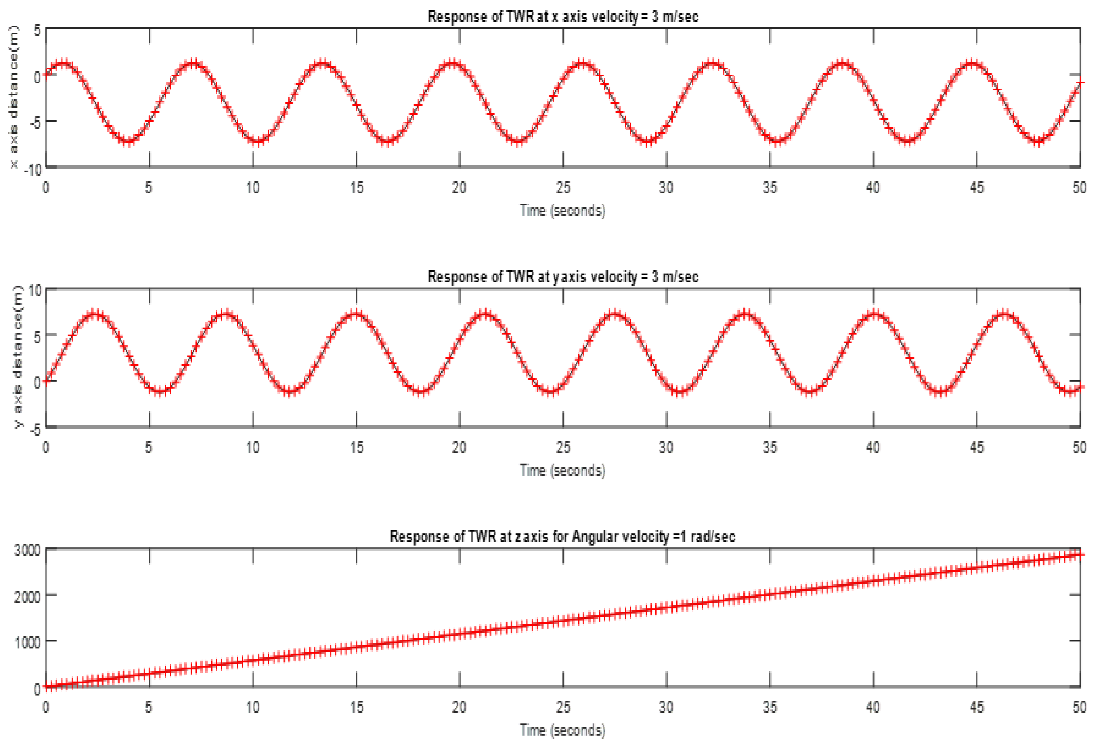
| Dataset 3 | 0 | 0 | 1 |
| Dataset 4 | 3 | 3 | 0.05 |
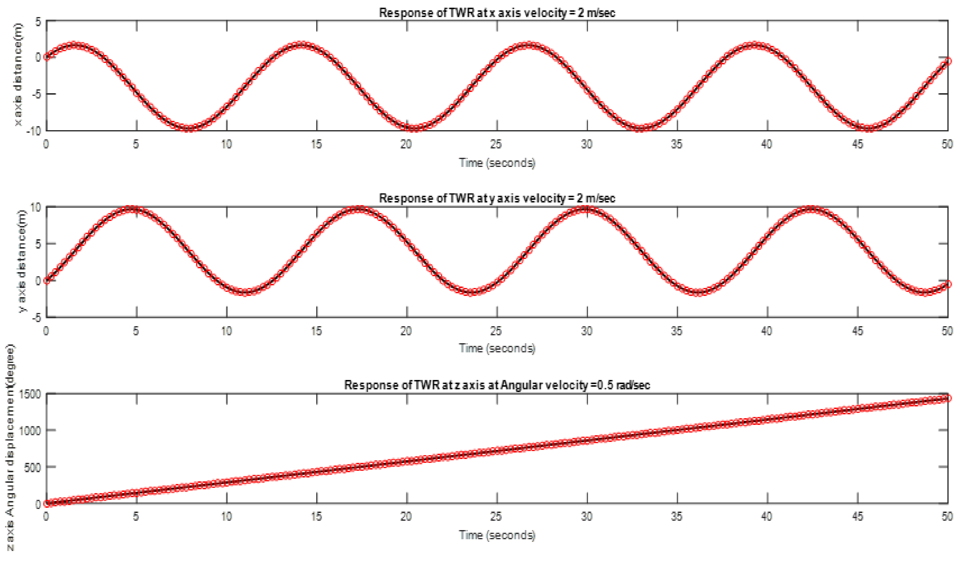
| Dataset 5 | 3 | 3 | 0.5 |
| Dataset 6 | 3 | 3 | 1 |
| Dataset 7 | 5 | 0 | 0.05 |
| Dataset 8 | 1 | 0 | 0.05 |
| Dataset 9 | 0 | 5 | 0.05 |
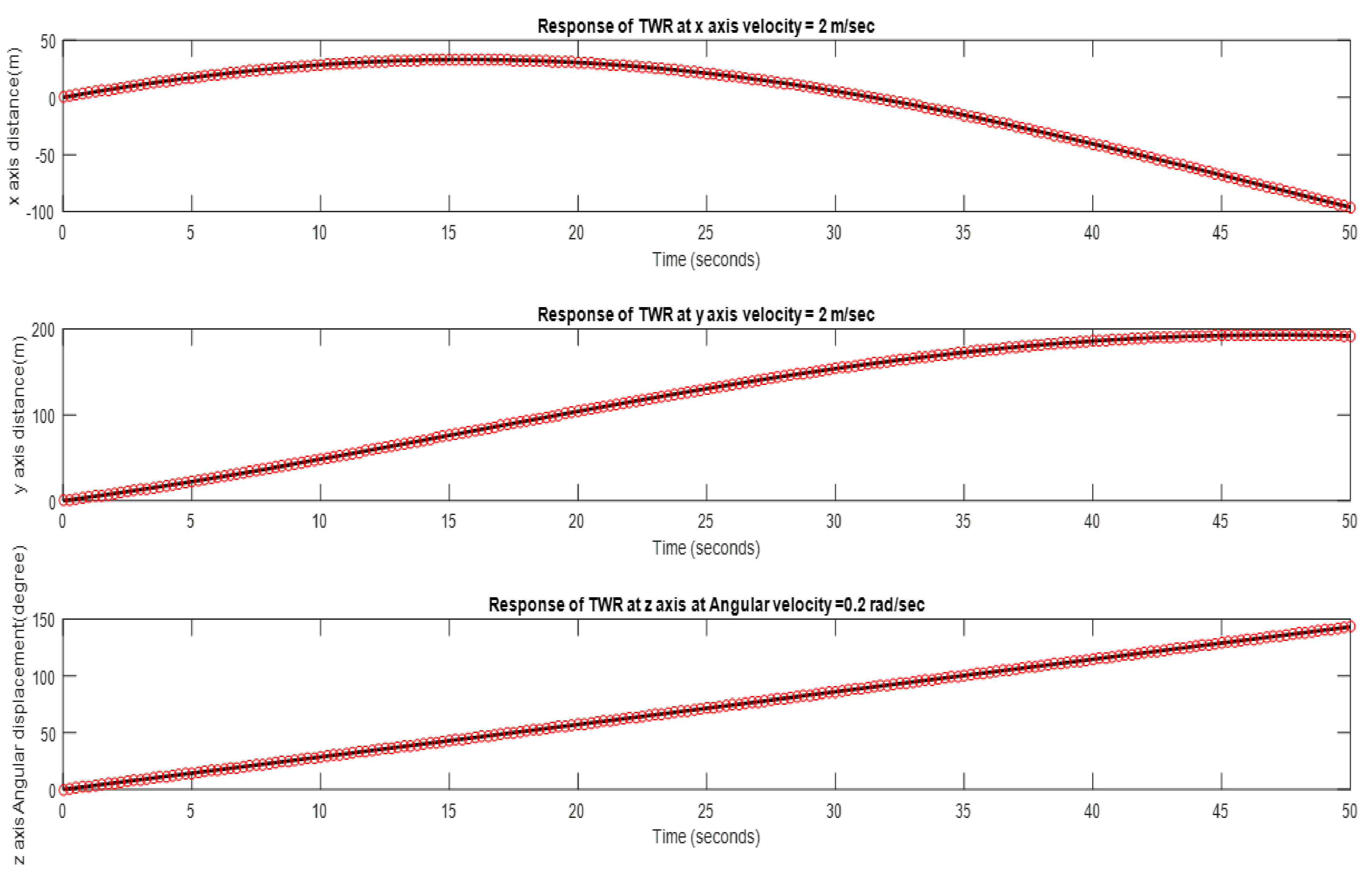
| Dataset 10 | 0 | 1 | 0 |
| Dataset 11 | 0.25 | 0.25 | 0.5 |
| Dataset 12 | 0.25 | 0.25 | 1 |
| Name of Dataset | Fit to Estimation Data (%) | Mean Square Error |
|---|---|---|
| Dataset 1 | 99.98 | |
| Dataset 2 | 99.99 | |
| Dataset 3 | 98.76 | |
| Dataset 4 | 99.98 | |
| Dataset 5 | 99.9 | 0.0001177 |
| Dataset 6 | 99.72 | 0.0002171 |
| Dataset 7 | 99.98 | |
| Dataset 8 | 99.93 | |
| Dataset 9 | 99.99 | |
| Dataset 10 | 99.98 | |
| Dataset 11 | 99.48 | |
| Dataset 12 | 98.76 |
Publisher’s Note: MDPI stays neutral with regard to jurisdictional claims in published maps and institutional affiliations. |
© 2022 by the authors. Licensee MDPI, Basel, Switzerland. This article is an open access article distributed under the terms and conditions of the Creative Commons Attribution (CC BY) license (https://creativecommons.org/licenses/by/4.0/).
Share and Cite
Khan, M.A.; Baig, D.-e.-Z.; Ashraf, B.; Ali, H.; Rashid, J.; Kim, J. Dynamic Modeling of a Nonlinear Two-Wheeled Robot Using Data-Driven Approach. Processes 2022, 10, 524. https://doi.org/10.3390/pr10030524
Khan MA, Baig D-e-Z, Ashraf B, Ali H, Rashid J, Kim J. Dynamic Modeling of a Nonlinear Two-Wheeled Robot Using Data-Driven Approach. Processes. 2022; 10(3):524. https://doi.org/10.3390/pr10030524
Chicago/Turabian StyleKhan, Muhammad Aseer, Dur-e-Zehra Baig, Bilal Ashraf, Husan Ali, Junaid Rashid, and Jungeun Kim. 2022. "Dynamic Modeling of a Nonlinear Two-Wheeled Robot Using Data-Driven Approach" Processes 10, no. 3: 524. https://doi.org/10.3390/pr10030524
APA StyleKhan, M. A., Baig, D.-e.-Z., Ashraf, B., Ali, H., Rashid, J., & Kim, J. (2022). Dynamic Modeling of a Nonlinear Two-Wheeled Robot Using Data-Driven Approach. Processes, 10(3), 524. https://doi.org/10.3390/pr10030524