Abstract
A new camera calibration technique based on serious distortion is proposed, which only requires the camera to observe the plane pattern in an arbitrary azimuth. It uses the geometrical imaging principle and radial distortion model to acquire radial lens distortion coefficient and the image coordinate (u0, v0), and then solves the linear equation aiming at the other parameters of the camera. This method has the following characteristics: Firstly, the position of the camera and the plane is arbitrary, and the technique needs only a single observation for plane pattern. Secondly, it is suitable for camera calibration with serious distortion. Thirdly, it does not need expensive ancillary equipment, accurate movement, or lots of photos observed from different orientations. Having been authenticated by computer emulation and actual experiment, the results of the proposed technique have proved to be satisfactory. The research has also paved a new way in camera calibration for further studies.
1. Introduction
Camera calibration is a necessary step in photogrammetry and computer vision, which plays an important role in many spheres such as 3D-measurement [1], 3D object reconstruction [2], robot navigation [3], visual surveillance [4], and industrial inspection [5]. Many studies have been conducted in this respect. And the techniques used can be classified into three categories: traditional camera calibration, active vision camera calibration, and camera self-calibration.
Traditional calibration. This kind of method uses information to gain parameters of the camera from the known landscape structure, which requires a calibration block of high precision. In 1986, Faugeras and Toscani [6] proposed a camera calibration method using some known points in the space to solve linear equations. Tsai [7] used the two-stage calibration technique to achieve the efficient computation of a camera’s external position and orientation. Further studies on two-stage calibration were carried out by Wen [8] and Gao [9]. These methods are always accurate for camera calibration; however, they do not fit in every situation.
Active vision camera calibration. This is completed based on the known information of the precise movement of a camera. Ma [10] exploited a sequence of specially designed motions, which were two groups of translational motions, to calibrate the camera. On this foundation, Yang [11] developed a new active vision calibration technique from four or five groups of the orthogonal motions. In recent years, active vision calibration has been developed further [12,13,14], which can easily solve problems and obtain parameters. This type of camera calibration method usually requires very sophisticated equipment and therefore calibration equipment is relatively expensive.
Camera self-calibration. This category only depends on the corresponding relationship among images, and does not need a calibration target, a known landscape structure, or the precise movement of the camera. There are two quadratic nonlinear constraints between two of the images. These constraints are composed of Kruppa equations and are used to obtain the intrinsic parameters of the camera [15,16]. Faced with the difficulty of obtaining nonlinear equations, scholars have proposed various methods for self-calibration of cameras [17,18,19]. The biggest advantage of the camera self-calibration technique is its excellent flexibility. Yet the robustness of it is lower and the nonlinear equations have to be solved.
Besides this, there are some other calibration methods which are calibrated by double planar mirrors [20], nonlinear optimization [21], feature Points Motions [22], the plane at infinity [23], invariance of cross-ratio [24], parallel circles [25], image information of different orientations from plane [26], coplanar camera calibration [27], planar mirrors from silhouettes [28], and turntable sequences from silhouettes [29].
Currently, camera calibration techniques are mainly focused on industrial cameras (they do not have severe camera distortion). However, wide-angle cameras (they have very bad camera distortion) are widely used in a number of specific fields due to the large field of view image information that can be obtained. An example is fruit tree branch-pruning robots [30], which require the acquisition of a complete image of a branch at close range and the identification of the branch to be cut from the overall branch image. Using a normal camera to capture images often requires multiple image stitches, which is not only time-consuming but also has a significant impact on stability and accuracy. Therefore, the use of a wide-angle camera to capture a complete image of the branch is a good option. Wide-angle camera lenses usually have severe distortion, and using traditional camera calibration methods to achieve wide-angle camera calibration usually requires human guidance and a lot of iterative processing to complete the calibration, which seriously affects the calibration efficiency and accuracy. To address these issues, this paper proposes a simple, fast, and intelligent wide-angle camera calibration method. The method is based on a planar target to complete the calibration of the camera. Compared with other methods, this method is simple to operate, has low equipment requirements, and only needs to acquire the target image once (traditional calibration based on a flat target requires multiple image acquisitions), has a small number of iterations (usually only ten), has a short computation time, and is suitable for the calibration of cameras with severe distortion.
The rest of the paper is organized as follows: Section 2 and Section 3 present a method of obtaining the image coordinate (u0, v0) and correcting the image distortion. In Section 4, we build the camera model, which includes four parameters, and we obtain all parameters of the camera. In Section 5, the experimental results are given. Finally, the results are analyzed and discussed in Section 6.
2. Obtaining the Image Coordinate (u0, v0) and Distortion Coefficients k1 and k2
In this paper, the image coordinate (u0, v0) is the key to the camera calibration, which can be gained exactly according to the following method.
2.1. Geometrical Deduction of Imaging
In a camera coordinate system, we assume there is an arbitrary line that has four points marked A, B, C, and D. Their imaging points are marked A′, B′, C′, D′ (see Figure 1a). In plane xcoczc, H1, H2, H3, H4, P1, P2, P3, and P4 are the projection points of A′, B′, C′, D′, A, B, C, and D (see Figure 1b).
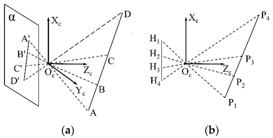
Figure 1.
The imaging principle of straight line is shown in two ways. In (a), it shows the corresponding relationship between the spatial line AB and the imaging line A′B′. In (b), the corresponding relationship in (Figure 1a) is projected onto the plane xcoczc. The plane α is the imaging plane.
As the spatial line AB is in the planar target, we can measure the distance between any two points in the line AB. Therefore, we can easily obtain the following ratios:
For the same line, the ratio of any two line segments does not change in the projection surface. According to (1) and (2), we have:
In Figure 1b, ZPi (i = 1, 2, 3, 4) and ZHi (i = 1, 2, 3, 4) are used to represent abscissa, while XPi (i = 1, 2, 3, 4) and XHi (i = 1, 2, 3, 4) are used to represent ordinate. Then we have:
The line P1P4 can be expressed as L1: X = kZ + b. Therefore, the coordinate of Pi (i = 1, 2, 3, 4) is represented as (ZPi, kZPi + b). To line HiPi, we have the equation of the straight line:
The line H1H4 and X-axis are parallel. Therefore, the line H1H4 can be expressed as L2: Z = n. According to (6), the ordinate of Hi (i = 1, 2, 3, 4) is (0, Xi).
From (5)–(7), we have
As can be seen from (8), the length ratio in the image is different from the actual one in the Euclidean Space, and it is related to the coordinate of P1, P2. For the same line, the projection won’t change the ratio between the segments. So B′C′/A′B′ = H2H3/H1H2, B′D′/A′B′ = H2H4/H1H2.
The following are transform relations of imaging point and image point.
From (8) and (9), we can find:
2.2. Calculation of the Ideal Image Coordinates without Distortion
In this paper, the actual image coordinates have serious distortion. However, the ideal image coordinates are very close to the actual image coordinates in the vicinity of (u0, v0), which is located near the center of the image. We try to make these points (A, B, C) near the center of the image when taking pictures. Point D is far away from point C and closest to the edge of the image. The image coordinates of A, B, and C are regarded as the ideal image coordinates without distortion, and are used in calculations. Because of the restriction in (10), we can find the relationship between ZP1 and ZP2.
From (10) and (11), we can obtain the provisional value of the ideal and undistorted image coordinates of point D.
Therefore, by using the above method, we can use some (at least three) line segments to obtain the ideal and undistorted image coordinates, which are on the edge of the image, marked (u′i, v′i) (i = 1, 2, 3, …).
2.3. Solving the Coordinate (u0, v0) and Distortion Coefficients k1 and k2
Camera lens aberration is mainly radial aberration. It to the optical axis centre point image coordinates as a reference point, and with the image point to the distance of the reference point into a non-linear relationship. Assuming that the camera in the image horizontal and vertical axis direction of the same aberration, the camera lens radial aberration model is as follows.
The (u, v) is an actual image coordinate, the (u0, v0) is the image coordinate of the central point of the optical axis, and the (u′, v′) is an ideal and undistorted image coordinate. are the second and fourth order radial distortion coefficients, respectively. Besides, r2 = (u′ − u0)2 + (v′ − v0)2. Using Equation (13), a number of distortion-free ideal image coordinates can be found. Substituting any two distortion-free ideal image coordinates , and the corresponding actual image coordinates , into Equations (4)–(7), where j, k = 1, 2, 3, …
In Equation (14), , , Solving for these yields.
These values of the parameters are only preliminary. However, putting them into (13), we can rectify the ideal and undistorted image coordinates, which is near the center of the image and considered identical with the actual image coordinates. The ideal and undistorted image coordinates of the points away from the central are obtained again, and are used for the calculation of the parameters.
In order to obtain more accurate image coordinates of the optical axis center point and aberration coefficient, more ideal image points without aberration need to be used, by combining two and two, and then using Equation (15) to find the parameters respectively. In order to ensure the stability of the parameters, the parameters can be obtained several times using different combinations and eventually obtaining the mean value of each parameter. The mean value of each parameter is obtained as follows.
In Equation (16), , , , and denote the value of the parameter for the qth combination, while , , , and denote the average value of each parameter. Since there is a difference between the actual image coordinates of the image point in the middle of the image and the ideal image coordinates without distortion, according to Equation (12), the actual image coordinates of the image point in the middle of the image need to be corrected, and the corrected image coordinates are used to find the ideal image coordinates without distortion away from the image center. Therefore, the actual image coordinates of , , , and the actual image coordinates of the image point in the middle of the image , and are substituted into Equation (13) to find the distortion-free ideal image coordinates , , and The above distortion-free ideal image coordinates are then used to obtain the coordinates of the distortion-free ideal image points away from the center of the image again. The average parameter values are obtained again using Equations (15) and (16). In order to obtain the exact parameters, several cycles are required until the parameters converge.
3. Image Distortion Correction
Because of the image distortion, it is difficult to make exact image information analysis. In view of this, we believe image correction is very necessary. From (13), we know that it is a dual higher order equation. Therefore, solving the ideal undistorted coordinates (u, v) directly is very difficult. According to u0, v0, k1, k2, and the image resolution ratio, we can estimate the coordinate range of the ideal and undistorted image points. In this range, an actual point corresponds to one or more ideal points. Thus, (13) is rewritten as follows.
The ideal and undistorted image points in estimated coordinate range are put into (17) in a certain order. Thus, we can obtain a series of real image coordinates. The ideal and undistorted image coordinates (1, 1), (1, 2) … (m, n) are used to calculate in (17), so the real image coordinates (u1, v1), (u2, v2) … (um, vn) are obtained. In other words, the corresponding ideal and undistorted image points of the real image coordinates (u1, v1), (u2, v2) … (um, vn) are found. In this way, one or more ideal and undistorted image points can correspond with a real image point. Therefore, this method is very simple without any additional processing.
4. Getting Other Parameters of Camera
An image point is denoted by [u, v]T, and the corresponding spatial point in the camera coordinate system is expressed as [xc, yc, zc]T. Min is the matrix of camera intrinsic parameters. Then we have
In the world coordinate system, the 3D point can be expressed as [xw, yw, zw]T. Because of the planar target, we assume: zw = 0. The cMw is the matrix of camera external parameters.
From (19), the results of calculation are as follows:
We assume:
According to (20) and (21), we can obtain the following equations:
From (22), through the elimination of zc, we have
We can use (xwi, ywi, 0) and (ui, vi) to represent the scene point in the world coordinate and image coordinate, and each of these points satisfies the Equation (23). Therefore, if there are n points, we will get the following equations set, which is composed of 2 × n equations:
In (24), with ,
,
When M′ = m/m33, (24) can be changed into (25).
Using the least square method, we have
The aij (i, j = 1, 2, 3) is used to represent the elements in the matrix M′. We have: aij = mij/m33. Using the relationship between (20) and (21), we can find aij = mij/pz and obtain the following equations.
Because the vectors [nx, ny, nz]T and [ox, oy, oz]T are unit vectors and orthogonal to each other. We have:
From (28), we can make an appropriate deformation.
Putting (27) into (29), we have
In (30), x = (1/kx)2, y = (1/ky)2, z = (1/pz)2, A1 = a11 − a31u0, B1 = a21 − a31v0, A2 = a12 − a32u0, B2 = a22 − a32v0. Because |D| ≠ 0, we have:
As the values of u0, v0 and M′ have been calculated in (15) and (26), putting these values into (31), we can obtain the values of x, y, and z. According to the camera imaging characteristics, we know the values of kx, ky, and pz are greater than zero. Therefore, it is not difficult to obtain the values of kx, ky, and pz by (30).
From (19) and (20), we can get the following relationship.
The matrix Min and matrix cMw are intrinsic and extrinsic parameter matrixes of the camera. The matrix Min contains four parameters, which are obtained in (15) and (32). Because the matrix Min has an inverse matrix, the intrinsic matrix cMw can be expressed as follows:
Based on the above derivation, the method described in this paper focuses on obtaining the ideal coordinates without distortion by means of the central reference point of the image and the projection principle, thus obtaining the parameters u0, v0, k1, k2 and ultimately the other parameters of the camera. This is shown in Figure 2.
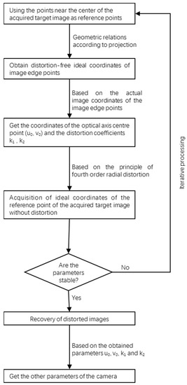
Figure 2.
This is the schematic diagram of the method described in this paper.
5. Experiments
5.1. Experimental Equipment
The main equipment for the ultra-wide-angle camera calibration experiments consisted of a Dell Inspion N4030 laptop, an ultra-wide-angle HD camera from Ryota Technology, a multi-square flat target calibration board, a fill light, a correction board, etc., as shown in the Figure 3. Figure 3a shows the laptop and the super wide angle camera, which are used for computer calibration processing and image acquisition, respectively. Figure 3b shows the multi-square flat target calibration board, which is the flat target for super wide angle camera calibration. Figure 3c shows the fill light, which is used for fill light processing when the target image is acquired. Figure 3d shows the aberration correction board, which is used for aberration correction experiments.
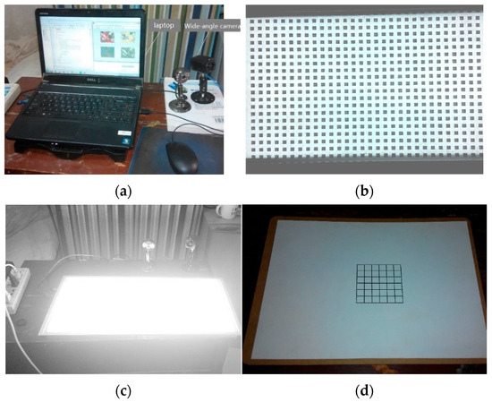
Figure 3.
This is the equipment used for calibration, where (a–d) are the experimental laptop and wide-angle camera, flat target, fill light, and correction plate, respectively.
5.2. Ultra-Wide-Angle Camera Calibration Process
The ultra-wide-angle camera calibration experiment consisted of the following processes.
- (1)
- Prepare a flat board of targets with equally spaced black squares.
- (2)
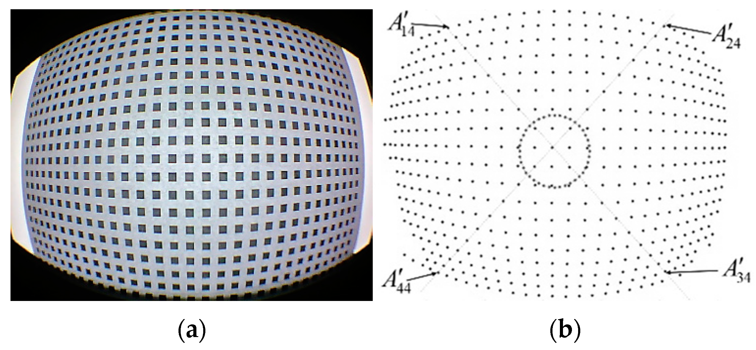
- The image of the target is captured at 1280 × 1024 pixels, as shown in Figure 4a.
 Figure 4. This is a flat target calibrated by the ultra-wide-angle camera, where (a) is the target image and (b) is the centroid image of the target square.
 - (3)
- The coordinates of the centroid of each black square in the target image were obtained using computer processing. In addition, a circular area is created with the centre of the image as the centre and 100 pixel points as the radius, and the coordinates of the centroids of all black squares within the circular area are obtained, as shown in Figure 4b.
- (4)
- The computer is used to find the combination of three points that satisfy in the same line, and to determine all other points on the same line that are far from the center of the image. Using Equation (12) to find the furthest ideal image coordinate points from the center without distortion, the image points found are shown in Figure 4b as , , and .
- (5)
- Combine the image points , , and in two according to Equation (15) to find the image coordinates (u0, v0) and the distortion coefficients k1 and k2. The values of and are then obtained according to the obtained parameters using Equation (16).
- (6)
- Using the average parameter values obtained, the image points on the line involved in the calculation are corrected according to Equation (17).
- (7)
- Repeat the steps 4, 5, and 6 until the desired parameters converge.
- (8)
- The camera is calibrated by using Equations (32)–(34) to find the other parameters of the camera based on the image coordinates of the optical axis center point and the distortion coefficient obtained.
- (9)
- The distorted image is corrected using the camera parameters acquired in step 8.
- (10)
- The camera calibration parameters were verified using the Zhang Zhengyou flat calibration method [26].
5.3. Results of Experiments
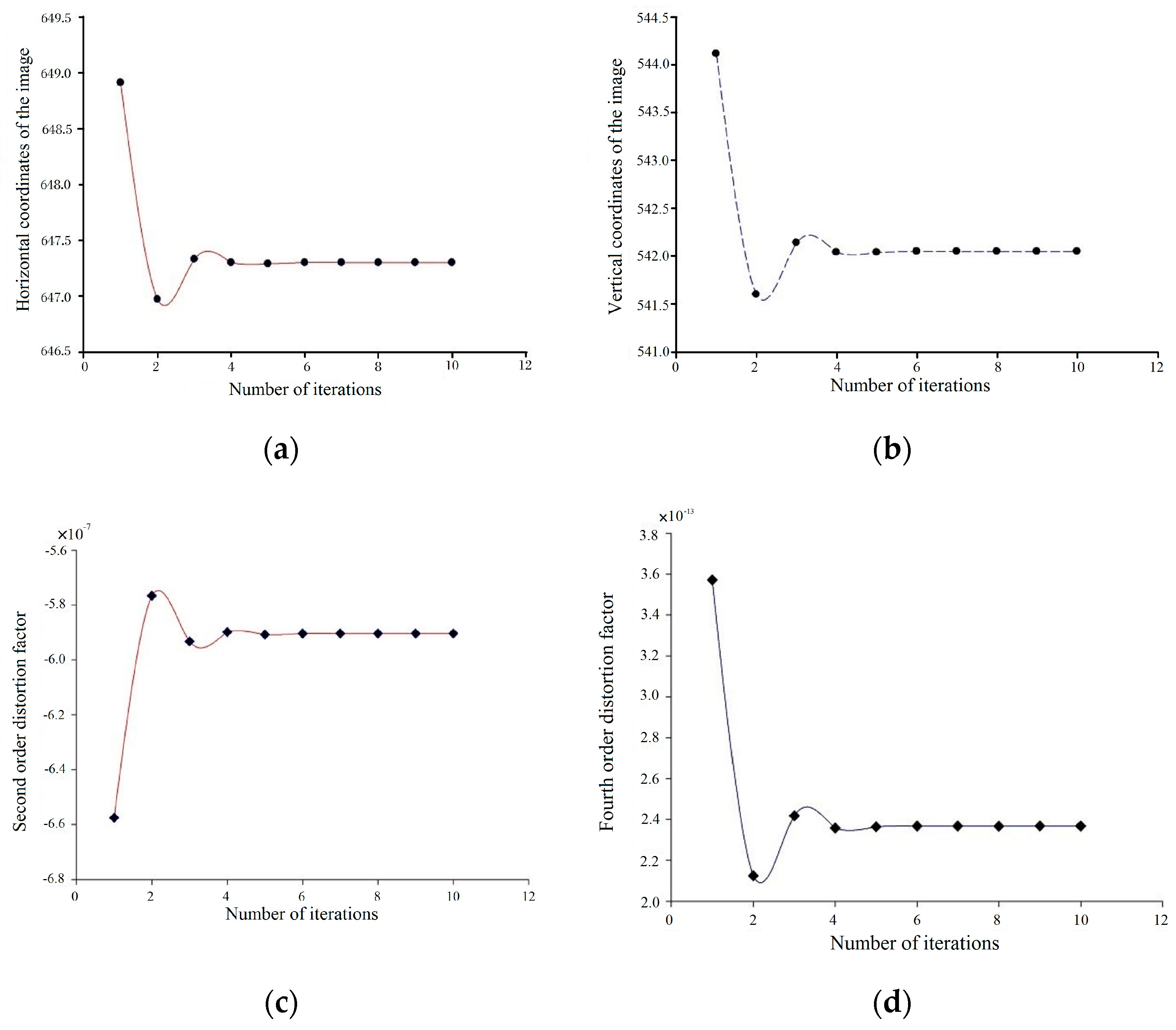
According to Equation (12) we can obtain the distortion-free ideal point image coordinates, and the relevant calculation results are shown in Table 1.We can easily find that the distortion-free ideal image coordinates of , , and gradually smooth out with the increase of the number of iterations. Using Equations (15) and (16), the and are found, as shown in Figure 5. According to the convergence relationship between the image coordinates of the distortion-free ideal point at the edge of the image, the image coordinates of the center point of the optical axis, the distortion coefficient and the number of iterations, it can be seen that and can be obtained exactly after only five iterations of calculation, so the whole processing process is very fast.

Table 1.
The relationship between coordinate parameters and iterations.
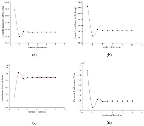
Figure 5.
These are the relations for the iterations involved within the camera, where (a–d) indicate the number of iterations with respect to u0, v0, k1, k2 respectively.
The final camera internal reference matrix and external reference matrix were obtained from the ultra-wide-angle camera calibration experiments as follows.
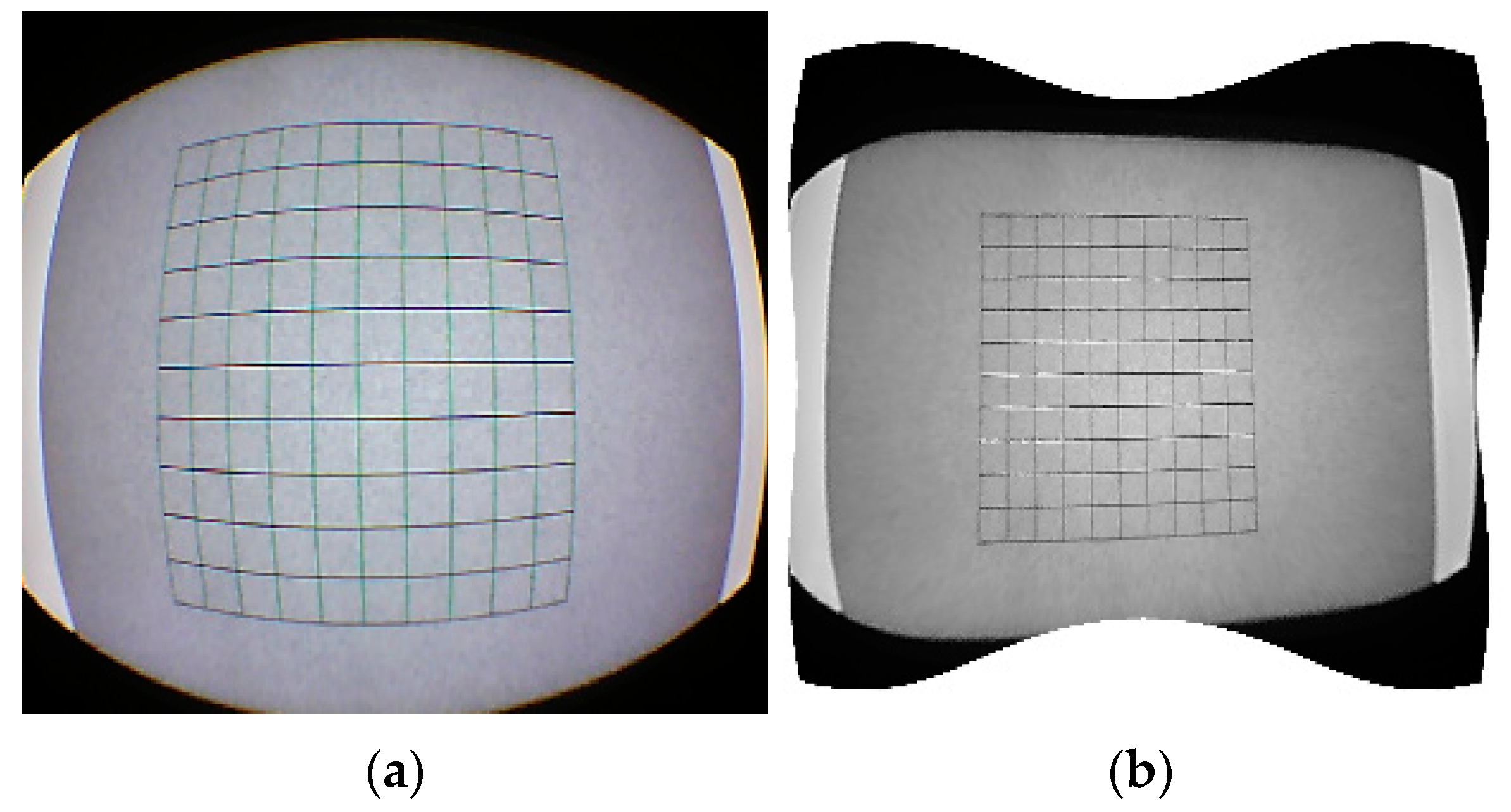
In this paper, the image correction is carried out according to the requested aberration coefficient and the image coordinates of the optical axis center point, and a good correction effect is obtained, as shown in Figure 6. This shows that the calibration method described in this paper has certain engineering application value.

Figure 6.
This is the image correction, where (a) is the distorted image and (b) is the corrected image of the distorted image.
A comparison of the camera parameters obtained in this paper with those obtained using Zhang’s calibration method is shown in Table 2. The comparison shows that the values obtained are consistent, indicating that the algorithm described in this paper is able to obtain more accurate camera parameters. Therefore, the calibration method for ultra-wide-angle cameras proposed in this paper has strong application value and can be further applied in industry and agriculture.
Table 2.
Comparison of the camera parameters with different algorithms.
6. Conclusions
In this paper, we have proposed a new calibration method, which is obviously different from others. In the experiment, this method has been tested from different observation angles and distances, and the results were satisfactory. Beginning with a few points in the center of the image, whose distortion is weaker, more accurate experimental data can be ensured. Therefore, the position of the planar plane is very important. In the experiment and simulation, the ratios of length are both D1B1:C1B1:B1A1 = 5.5:1:1 and are considered reasonable in the experiment. To obtain accurate data, more points are added in the planar plane, and repeated experiments have been carried out.
This method is suitable for a camera with obvious distortion, and only requires the camera to take one picture in a certain position. In addition, the algorithm described in this paper requires only one image acquisition for the entire calibration process, and after the image is acquired, no manual identification or guidance is required, and the ultra-wide-angle camera calibration can be automated by a computer program. In addition, only the aberration parameters and the image coordinates of the optical axis center point are iteratively calculated during the calculation process, and the number of iterations is low, making the whole calibration process faster than Zhang’s calibration method. As can be seen, the specific advantages of the algorithm proposed in this paper include the following.
- (1)
- Only one image acquisition of the target is required.
- (2)
- No expensive ancillary equipment is required and it is highly adaptable.
- (3)
- High calibration progress within 1% relative error.
- (4)
- Rapid calibration.
Therefore, the algorithm proposed in this paper has strong application value and is suitable for promotion in the field of robot vision in agriculture and industry.
Author Contributions
Conceptualization, B.H.; Formal analysis, S.Z.; Methodology, B.H.; Writing–original draft, S.Z.; Writing–review & editing, B.H. All authors have read and agreed to the published version of the manuscript.
Funding
The project is supported by the Science and Technology Plan Project of Guizhou Province (Grant No. QKHJC [2019]1152) and High-level Talents Research Initiation Fund of Guizhou Institute of Technology (Grant No. XJGC20190927).
Institutional Review Board Statement
This study does not involve human or animal research and does not require ethical approval.
Informed Consent Statement
This study does not involve human or animal research and does not require ethical approval.
Data Availability Statement
The study did not report data.
Acknowledgments
We would like to thank every member of the research group for their support and help. We would also like to thank Yi Peng, Gongpeng Dai and Haixia. They give great advice for this paper.
Conflicts of Interest
The authors declare no conflict of interest.
References
- Higuchi, H.; Fujii, H.; Taniguchi, A.; Watanabe, M.; Yamashita, A.; Asama, H. 3D Measurement of Large Structure by Multiple Cameras and a Ring Laser. J. Robot. Mechatron. 2019, 31, 251–262. [Google Scholar] [CrossRef]
- Han, X.-F.; Laga, H.; Bennamoun, M. Image-Based 3D Object Reconstruction: State-of-the-Art and Trends in the Deep Learning Era. IEEE Trans. Pattern Anal. Mach. Intell. 2021, 43, 1578–1604. [Google Scholar] [CrossRef] [PubMed] [Green Version]
- Chae, H.-W.; Choi, J.-H.; Song, J.-B. Robust and Autonomous Stereo Visual-Inertial Navigation for Non-Holonomic Mobile Robots. IEEE Trans. Veh. Technol. 2020, 69, 9613–9623. [Google Scholar] [CrossRef]
- Tarrit, K.; Molleda, J.; Atkinson, G.A.; Smith, M.L.; Wright, G.C.; Gaal, P. Vanishing point detection for visual surveillance systems in railway platform environments. Comput. Ind. 2018, 98, 153–164. [Google Scholar] [CrossRef]
- Ali, M.A.H.; Lun, A.K. A cascading fuzzy logic with image processing algorithm–based defect detection for automatic visual inspection of industrial cylindrical object’s surface. Int. J. Adv. Manuf. Technol. 2019, 102, 81–94. [Google Scholar] [CrossRef]
- Faugeras, O.; Toscani, G. The calibration problem for stereo. In Proceedings of the IEEE Computer Society Conference on Computer Vision and Pattern Recognition, Miami Beach, FL, USA, 22–26 June 1986; pp. 15–20. [Google Scholar]
- Tsai, R. A versatile camera calibration technique for high-accuracy 3D machine vision metrology using off-the-shelf TV cameras and lenses. IEEE J. Robot. Autom. 1987, 3, 323–344. [Google Scholar] [CrossRef] [Green Version]
- Weng, J.; Cohen, P.; Herniou, M. Camera calibration with distortion models and accuracy evaluation. IEEE Trans. Pattern Anal. Mach. Intell. 1992, 14, 3965–3980. [Google Scholar] [CrossRef] [Green Version]
- Gao, H.; Wu, C.; Gao, L.; Li, B. An improved two-stage camera calibration method. In Proceedings of the 2006 6th World Congress on Intelligent Control and Automation, Dalian, China, 21–23 June 2006; Volume 1–12, pp. 9514–9518. [Google Scholar]
- Ma, S. A self-calibration technique for active vision systems. IEEE Trans. Robot. Autom. 1996, 12, 114–120. [Google Scholar]
- Yang, C.; Wang, W.; Hu, Z. An active vision based camera intrinsic parameters self-calibration technique. Chin. J. Comput. 1998, 21, 428–435. [Google Scholar]
- Gibbs, J.A.; Pound, M.P.; French, A.P.; Wells, D.M.; Murchie, E.H.; Pridmore, T.P. Active Vision and Surface Reconstruction for 3D Plant Shoot Modelling. IEEE/ACM Trans. Comput. Biol. Bioinform. 2019, 17, 1907–1917. [Google Scholar] [CrossRef]
- Xu, D.; Zhang, D.; Liu, X.; Ma, L. A Calibration and 3-D Measurement Method for an Active Vision System with Symmetric Yawing Cameras. IEEE Trans. Instrum. Meas. 2021, 70, 1–13. [Google Scholar] [CrossRef]
- Xu, G.; Chen, F.; Li, X.; Chen, R. Closed-loop solution method of active vision reconstruction via a 3D reference and an external camera. Appl. Opt. 2019, 58, 8092–8100. [Google Scholar] [CrossRef] [PubMed]
- Faugeras, O.; Luong, Q.; Maybank, S. Camera self-calibration: Theory and experiments. In Proceedings of the 2nd European Conference on Computer Vision, Margherita Ligure, Italy, 19–22 May 1992; pp. 321–334. [Google Scholar]
- Maybank, S.; Faugeras, O. A theory of self-calibration of a moving camera. Int. J. Comput. Vis. 1992, 8, 123–151. [Google Scholar] [CrossRef]
- Yuan, C.; Liu, X.; Hong, X.; Zhang, F. Pixel-Level Extrinsic Self Calibration of High Resolution LiDAR and Camera in Targetless Environments. IEEE Robot. Autom. Lett. 2021, 6, 7517–7524. [Google Scholar] [CrossRef]
- Guan, B.; Yu, Y.; Su, A.; Shang, Y.; Yu, Q. Self-calibration approach to stereo cameras with radial distortion based on epipolar constraint. Appl. Opt. 2019, 58, 8511–8521. [Google Scholar] [CrossRef]
- Liu, S.; Peng, Y.; Sun, Z.; Wang, X. Self-calibration of projective camera based on trajectory basis. J. Comput. Sci. 2018, 31, 45–53. [Google Scholar] [CrossRef]
- Zhao, Y.; Li, Y. Camera self-calibration from projection silhouettes of an object in double planar mirrors. J. Opt. Soc. Am. A Opt. Image Sci. Vis. 2017, 34, 696. [Google Scholar] [CrossRef]
- Führ, G.; Jung, C.R. Camera Self-Calibration Based on Nonlinear Optimization and Applications in Surveillance Systems. IEEE Trans. Circuits Syst. Video Technol. 2015, 27, 1132–1142. [Google Scholar] [CrossRef]
- Sun, J.; Wang, P.; Qin, Z.; Qiao, H. Effective self-calibration for camera parameters and hand-eye geometry based on two feature points motions. IEEE/CAA J. Autom. Sin. 2017, 4, 370–380. [Google Scholar] [CrossRef]
- El Akkad, N.; Merras, M.; Baataoui, A.; Saaidi, A.; Satori, K. Camera self-calibration having the varying parameters and based on homography of the plane at infinity. Multimed. Tools Appl. 2018, 77, 14055–14075. [Google Scholar] [CrossRef]
- Wan, B.; Zhang, D. Calibration method of camera intrinsic parameters with invariance of cross-ratio. Comput. Eng. 2008, 34, 261–262. [Google Scholar]
- Wu, Y.; Zhu, H.; Hu, Z.; Wu, F. Camera calibration from the quasi-affine invariance of two parallel circles. In Proceedings of the 8th European Conference on Computer Vision, Prague, Czech Republic, 11–14 May 2004; Volume 3021, pp. 190–202. [Google Scholar]
- Zhang, Z. A flexible new technique for camera calibration. IEEE Trans. Pattern Anal. Mach. Intell. 2000, 22, 1330–1334. [Google Scholar] [CrossRef] [Green Version]
- Chatterjeel, C.; Roychowdhury, V. Algorithms for coplanar camera calibration. Mach. Vis. Appl. 2000, 12, 84–97. [Google Scholar] [CrossRef]
- Ying, X.; Peng, K.; Hou, Y.; Guan, S.; Kong, J.; Zha, H. Self-Calibration of Catadioptric Camera with Two Planar Mirrors from Silhouettes. IEEE Trans. Pattern Anal. Mach. Intell. 2013, 35, 1206–1220. [Google Scholar] [CrossRef]
- Zhang, H.; Wong, K. Self-Calibration of Turntable Sequences from Silhouettes. IEEE Trans. Pattern Anal. Mach. Intell. 2009, 31, 5–14. [Google Scholar] [CrossRef] [Green Version]
- Biao, H.; Ming, S.; Lei, S. Vision recognition and framework extraction of loquat branch-pruning robot. J. South China Univ. Technol. Nat. Sci. 2015, 43, 114–119, 126. [Google Scholar]


Publisher’s Note: MDPI stays neutral with regard to jurisdictional claims in published maps and institutional affiliations. |
© 2022 by the authors. Licensee MDPI, Basel, Switzerland. This article is an open access article distributed under the terms and conditions of the Creative Commons Attribution (CC BY) license (https://creativecommons.org/licenses/by/4.0/).