Prediction-Interval-Based Credibility Criteria of Prognostics Results for Practical Use

Abstract

Prognostics is an AI-based technique for predicting the degrading/damaging behavior and remaining useful life (RUL) of a system, which facilitates a cost-effective and smart maintenance process. Many prognostics methods have been developed for various applications, such as bearings, aircraft engines, batteries, and fuel cell stacks. Once a new prognostics method is developed, it is evaluated using several metrics based on the true value of the RUL. However, these typical evaluation metrics are not applicable in real-world applications, as the true RUL cannot be known before the actual failure of a system. There are no ways to determine the reliability of prognostics results in practice. Therefore, this article presents the credibility criteria of prognostics results based on prediction intervals (PI), which are known values, unlike the true RUL. The PI-based credibility criteria for prognostics results are explained with two simple examples under different levels of noise to help with the decision making on prognostics results in the industrial field.

1. Introduction

Prognostics is one of the disciplines in condition-based maintenance [1], which is a cost-effective maintenance strategy that repairs damaged parts only when required. The purpose of prognostics is to predict the remaining useful life (RUL) of the system, which is defined as the remaining cycles/time before maintenance and has been studied for the past few decades in many engineering applications, such as bearings [2,3], aircraft engines [4], batteries [5], and fuel cell stacks [6]. RUL can be predicted using degradation data obtained up to the current time and several prediction algorithms, such as particle filters [7,8] and artificial neural networks [9,10].

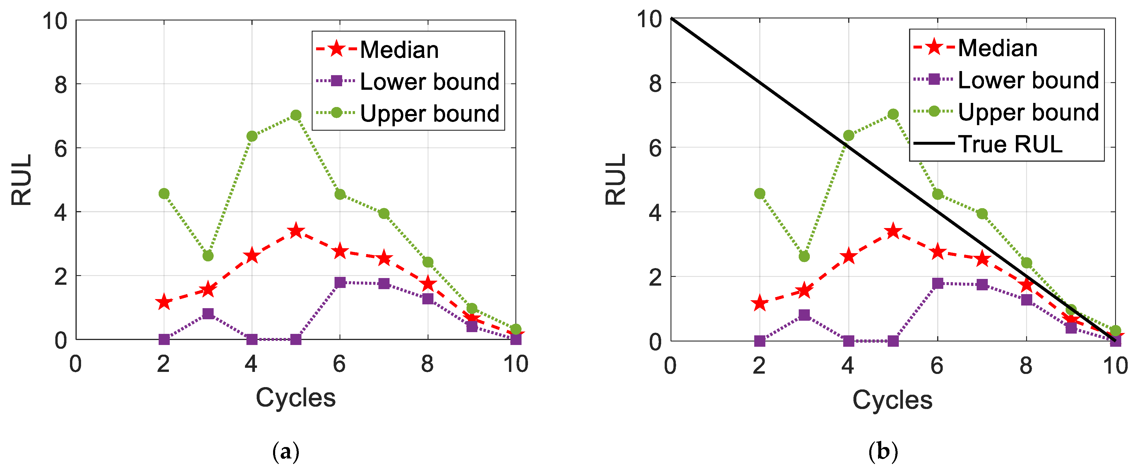
The results of RUL prediction are updated whenever new measurement data are available during the life span of a system; an instance of such a system is illustrated in Figure 1. In Figure 1a, pentagrams, squares, and circles represent the median, lower bound, and upper bound of the RUL prediction results, respectively. We assume that this system has been operating for two cycles as of now. In this case, the median RUL (the pentagram at two cycles in Figure 1a) indicates that this system needs maintenance approximately one cycle later. Thereafter, this system is operated for one more cycle, and the current duration becomes three cycles. It is found that maintenance is not necessary, and the median of RUL prediction is even increased to approximately one and a half cycles. The RUL is the remaining number of cycles and should thus decrease as the operating cycles of the system increases; however, the prediction results show an increasing tendency of up to five cycles. Although RUL prediction results decrease after one cycle, that is, the current duration is six cycles, there is no way to determine the reliability of the current prediction result by only knowing the past prediction results (note that the RUL results after the current six cycles are unknown as of now). A typical way to evaluate the performance of RUL prediction is to employ the true value of the RUL, as shown in Figure 1b. The solid diagonal line is the true RUL, and it is now clear whether the prediction results are reliable.

The metrics based on the true value are not limited to prognostics and are widely used in every field when performance evaluation is required. Orozco-Arias et al. (2020) compared 26 different performance metrics used in bioinformatics, such as accuracy, precision, and F1-score; these metrics were based on the true value, such as the true sample size [11]. In addition, Foit et al. (2020) addressed the overall equipment efficiency metrics for transport facilities, and true values, such as real cycle time and real number of good quality products, were required for metrics [12]. It is expected that the true value can be employed to evaluate the performance of the developed methods. With the growth in developing prognostics methods, not only basic error calculation, but also metrics for prognostics [13] were presented to evaluate the performance of developed prognostics methods. Since then, prognostics metrics have been commonly employed in many related studies [14,15,16].

However, the true value of RUL is known only when a system reaches its end of life (EOL). In other words, the solid diagonal line in Figure 1b can be drawn at 10 cycles; thus, the RUL results are obtained in the real world, as shown in Figure 1a. Without the true value, there are no methods for determining the reliability of the prediction results. Of course, the prediction results from the thoroughly validated method are reliable, but not always. The prediction results are also affected by the quality of the data, for example, the number, noise level, and damage growth rate. It is still unclear which results are reliable without the true value. This unconfirmed reliability of the prediction results might be one of the reasons why industrial companies are interested in but not enthusiastic about prognostics.

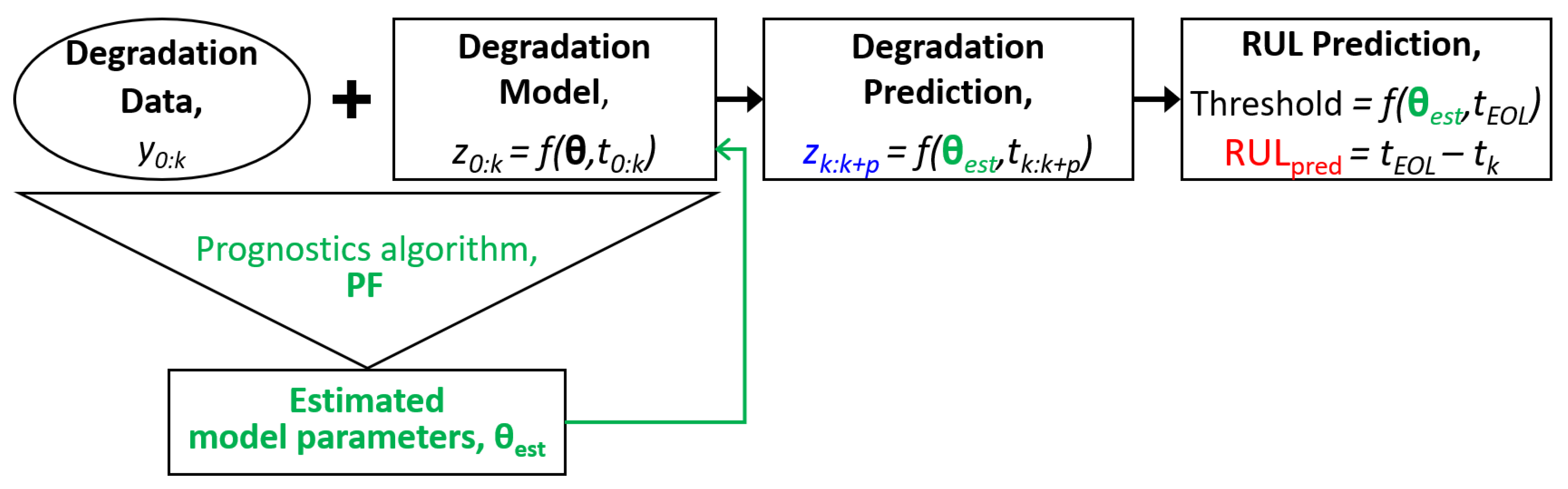
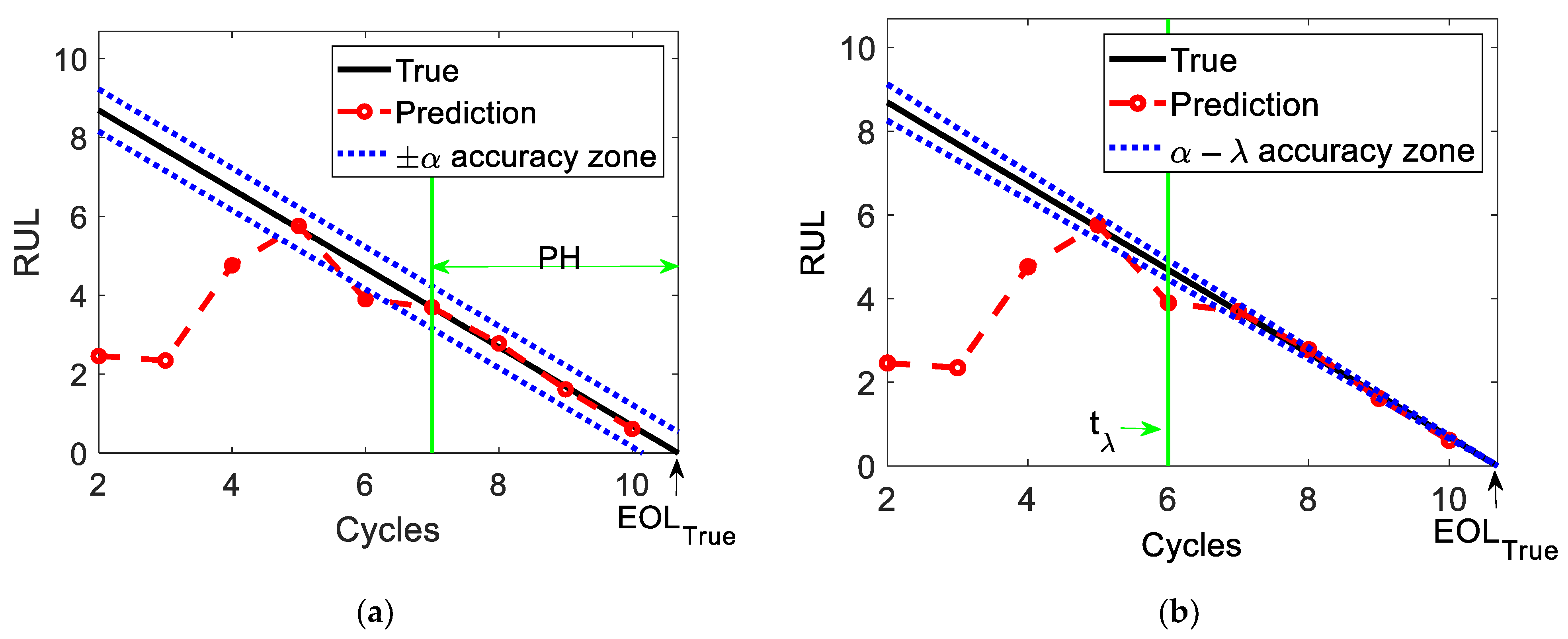
In this article, the credibility criteria of the prognostics results are presented as a guideline for decision making without the true RUL in the real world. The criteria are based on the fundamental phenomenon that a prediction interval (PI) is narrower as more data are used. PI is the difference between the lower and upper bounds of the RUL prediction (refer to Figure 1). Additionally, there is another type of PI in prognostics results, which is comprehensively explained in Section 2 and Section 3. Since the PI-based credibility criteria are graphically expressed with two types of PIs, they are simple, intuitive, and practical.

This article is organized as follows: in Section 2, the general prognostics process is introduced with the typical performance evaluation metrics; in Section 3, the credibility criteria of prognostics results are presented based on the PI; in Section 4, crack growth and battery degradation examples are employed to validate the proposed criteria; in Section 5, the study is concluded.

2. General Prognostics Process and Evaluation Metrics

2.1. General Prognostics Process

Prognostic methods are typically classified into physics-based, data-driven, and hybrid approaches. The main difference between the physic-based and data-driven approaches is the availability of a physical degradation model. When a physical model describing the degradation behavior of a system is available, the prognostics method can be considered the parameter estimation method of the curve-fitting problem in the extrapolating region. Among several physics-based prognostics algorithms, the particle filter (PF) [7,8] is commonly used. On the other hand, a data-driven approach is employed when a physical degradation model is unavailable. In this case, the best mathematical model and the optimal parameters pertaining to the model are simultaneously determined. Artificial neural networks [9,10] are commonly used in data-driven approaches. Finally, hybrid approaches combine the above-mentioned two methods to improve prediction performance.

Regardless of the various approaches, the general process of the prognostics methods is basically the same, except for the availability of a physical degradation model. As the physics-based approach is simpler and clearer than the other two approaches, it is employed in this study, as illustrated in Figure 2. The prerequisite condition for prognostics is the degradation data, such as the crack size, battery capacity, wear volume, and extracted features from the sensor signals. The degradation data (y) obtained up to the current time (t_k) are combined with a degradation model (z, physical or mathematical model) to identify the model parameters ($\mathsf{\theta }$) in the prognostics algorithm, such as PF. The estimated model parameters are used to predict the future degradation behavior (z_k+p) until the degradation reaches the failure threshold for maintenance. The time when the degradation reaches the threshold is the EOL, and the RUL is obtained by subtracting the current time from the EOL.

The prognostic results for the current cycle are illustrated in Figure 3 as an example. The black dot markers are the degradation data that were measured nine times up to the current cycle. Since there are several sources of uncertainty in the prognostics process caused by measurement and algorithm errors, the degradation behavior and RUL are predicted as distributions, as shown in the PDF curves in Figure 3. The degradation distribution at the current cycle is propagated, as depicted by the blue dashed curves, which are the lower and upper bounds of the prediction results of the degradation behavior. The cycle wherein the degradation prediction reaches the failure threshold (green horizontal line) is a predicted EOL, and RUL (red PDF) is predicted by subtracting the current cycle from the EOL.

In the method development stage, the performance of RUL prediction is evaluated. Existing metrics to evaluate prognostics performance are briefly introduced in the next section.

2.2. Metrics for Evaluating Prognostics Performance

The most common metric used in every field is to calculate the accuracy or error of the results. The relative error (RE) is one of the frequently used metrics, which is expressed as follows in terms of prognostics:

$$\mathrm{RE}=\left|\frac{{\mathrm{RUL}}_{\mathrm{True}}-{\mathrm{RUL}}_{\mathrm{Predi}}}{{\mathrm{RUL}}_{\mathrm{True}}}\right|$$

(1)

where ${\mathrm{RUL}}_{\mathrm{Ture}}$ and ${\mathrm{RUL}}_{\mathrm{Predi}}$ are the true and predicted RUL, respectively. RE is the error of the RUL prediction result relative to the true value at the prediction point. Another frequently used metric is the root mean square error (RMSE) defined as follows:

$$\mathrm{RMSE}=\sqrt{\frac{1}{n}{{\displaystyle \sum }}_{i=1}^n{d}_i^2},$$

(2)

where $d_i={\mathrm{RUL}}_{\mathrm{True}}-{\mathrm{RUL}}_{\mathrm{Predi}}$ at the ith cycle for RUL prediction, and n is the total number of predictions during the entire life of a system. This is a type of average cumulative error.

There are performance evaluation metrics specialized in prognostics [13], which contains five metrics: prognostic horizon, $\mathsf{\alpha }-\mathsf{\lambda }$ accuracy, relative accuracy, cumulative relative accuracy, and convergence. The prognostic horizon (PH) is the difference between the true EOL and the first time the prediction result continuously resides in the accuracy zone (arbitrary ratio to the true EOL), as shown in Figure 4a. A longer PH indicates a better performance. $\mathsf{\alpha }-\mathsf{\lambda }$ accuracy determines whether a prediction result falls within the $\mathsf{\alpha }$ accuracy zone (arbitrary ratio to the true RUL) at a specific cycle $t_{\lambda }$, as shown in Figure 4b. The results yield ‘true (within the accuracy zone)’ or ‘false.’ Relative accuracy is the same as $1-\mathrm{RE}$ in Equation (1), and cumulative relative accuracy is the average of the relative accuracies obtained during the life span of a system. Finally, convergence represents the convergence speed by calculating the center of mass of the area under the error curve, which can be obtained based on $\mathrm{RE}$ in Equation (1).

In addition to the aforementioned metrics, most performance evaluation metrics require the true value of RUL. These approaches are necessary for developing and validating new methods but they cannot be practically applied. The true value of RUL is the future value; thus, it can never be known until the failure of a system actually occurs. If this is the case, is trusting the prediction results given by the best method evaluated during the developing stage the only way? Once the method has been thoroughly validated, it is likely to work well in the practical stage. However, the accuracy of the prediction results can vary with the quality of the data, for example, the number, nose level, and damage growth rate. Therefore, in the next section, PI-based credibility criteria are presented to provide guidelines on the reliability of the prediction results without a true value.

3. PI-Based Credibility Criteria of Prognostics Results

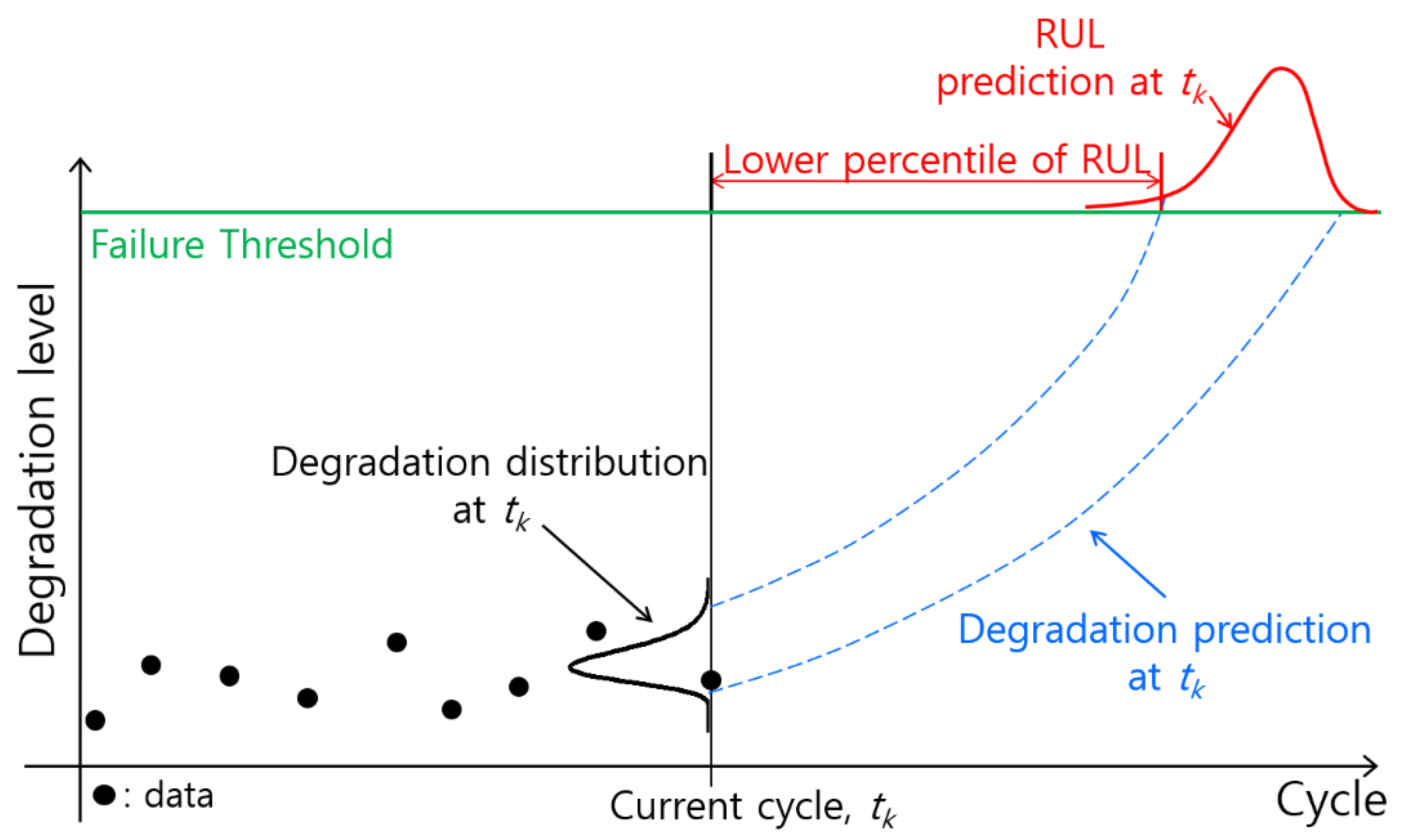
The credibility criteria are to make a decision on how reliable the prognostics results are, which are based on the fact that PI decreases as more data are used. While the true RUL, which is a prerequisite for conventional evaluation methods, is never known as long as the system functions properly, PI is a practical value obtained at every prediction cycle.

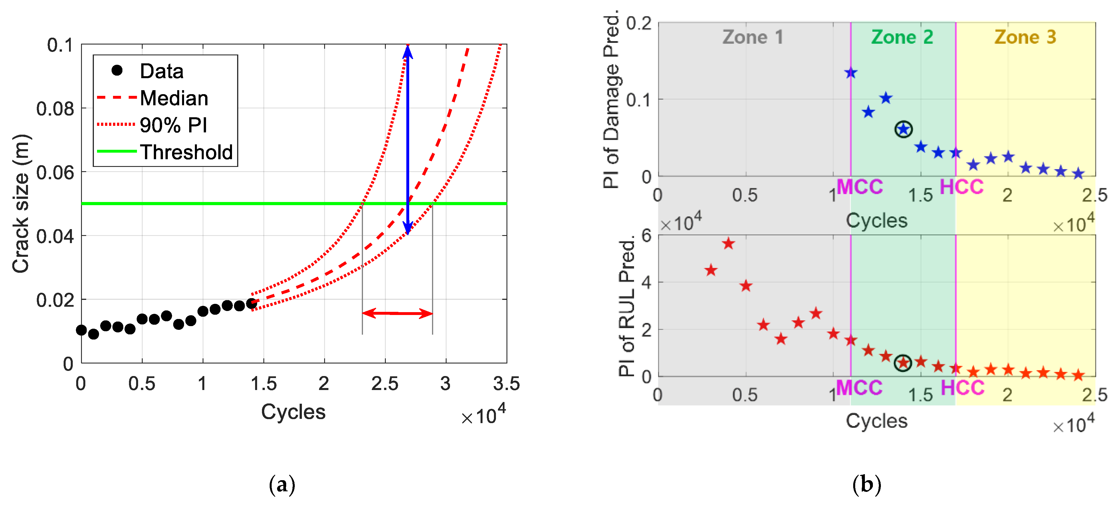
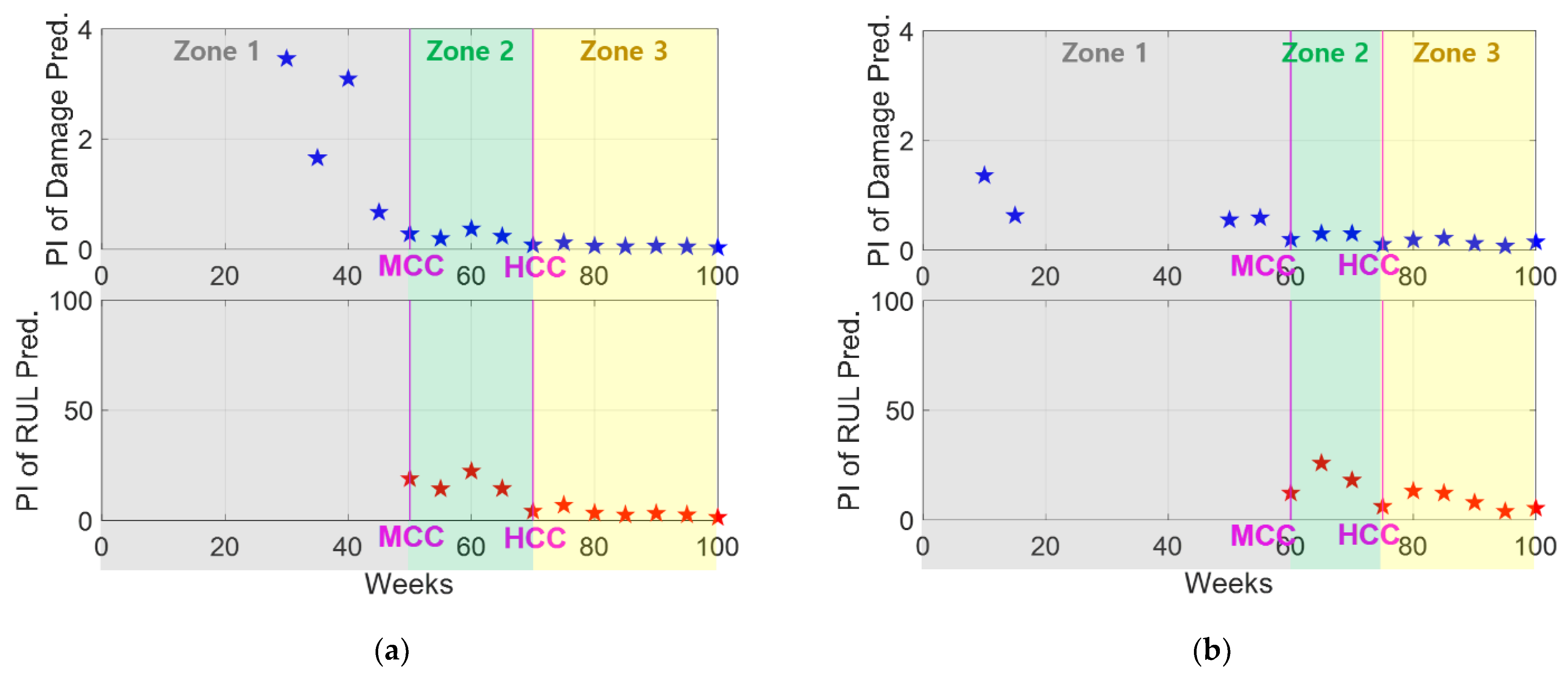
There are two types of PI in the results of prognostics, i.e., one from the damage and other from RUL prediction results, which are depicted in Figure 5a. In the figure, the black dots are the measurement data, the red dashed and dotted curves are the median and the lower/upper bounds of the damage prediction result, respectively, and the green horizontal line is a threshold. The cycle in which the damage prediction curves reach the threshold is the predicted EOL. The predicted RUL is obtained by subtracting the current 14,000 cycles from the predicted EOL. The PI of the RUL is indicated by the red horizontal arrow in Figure 5a, which is marked as the red pentagram in the black circle in Figure 5b. In addition, the PI of damage is obtained at the point where the median (red dashed curve) reaches the threshold, which is depicted by the blue vertical arrow in Figure 5a and marked as the blue pentagram in a black circle in the upper part of Figure 5b.

The PIs for the credibility criteria marked as pentagrams in Figure 5b are obtained by repeating the prognostics process in Figure 5a at every measurement cycle. The credibility criteria are composed of three zones divided into two criteria: medium credibility criterion (MCC) and high credibility criterion (HCC), as shown in Figure 5b. MCC is the first cycle when reasonable values are obtained for both the damage and RUL PIs. In Figure 5b, the reason for the lack of markers for PI of damage is that the unfeasible results, that is, infinity or an unreasonable level of intervals, are obtained because of insufficient information (the number of data and damage growth rate), compared to the level of noise in the data. HCC is the first cycle where the PIs of both the damage and RUL simultaneously decrease three times continuously after MCC. This ‘three continuous times’ may not be absolute but is a general stability standard.

Based on these two criteria points, zones 1, 2, and 3 are defined as before MCC, between MCC and HCC, and after HCC, respectively. When the prognostics results are in Zone 1, they are not feasible because of the lack of data to predict the degradation behavior and RUL. In contrast, zones 2 and 3 are feasible regions for making decisions based on the prognostics results. Zone 2 (between MCC and HCC) is a feasible region, but the prediction results can be significantly improved with more data because there are still several sources of uncertainty caused by the amount of data, damage growth rate, and inherent noise in the data. In a relative sense, Zone 3 (after HCC) reflects mostly inherent noise in the data (assuming there is no uncertainty in the prediction algorithm) and thus has a high level of credibility. The aforementioned characteristics of the credibility zones are summarized in

Table 1. Characteristic of the credibility zones.

Criterion		Level of Credibility	Note	Information to Noise Level in Data
MCC	Zone 1 (before MCC)	Very low	Not feasible	Insufficient
	Zone 2 (between MCC and HCC)	Medium	Feasible, but considering uncertainties	Moderate
HCC
	Zone 3 (after HCC)	High	Feasible	Sufficient (inherent noise in data)

MCC: the first cycle when reasonable values are shown in both the damage and RUL intervals. HCC: the first cycle when the PIs of both the damage and RUL simultaneously decrease three continuous times.

.

4. Case Study for Validation

The PI-based credibility criteria are based on known information from the past to the present, and any future information, such as a true RUL, is not employed. Therefore, it is validated whether the credibility classification from the PI-based criteria is appropriate using two different examples.

4.1. Crack Growth Problem

It is assumed that a crack is detected in the fuselage panel under repeated pressurization loading. The size of this crack increases as the operating cycle of the aircraft increases, and its growth behavior can be expressed using the Paris model [17] as

$$\frac{da}{dN}=C{\left(\Delta K\right)}^m,\Delta K=\Delta \sigma \sqrt{\pi a},$$

(3)

where a is the crack size, N is the number of operating cycles, m and C are the model parameters to be found, $\Delta K$ is the range of the stress intensity factor, and $\Delta \sigma$ is the stress range due to the pressure differential. Since the current damage size is expressed by the previous damage size in the PF, Equation (3) should be rewritten in the form of the crack transition function as

$$a_k=C_k{\left(\Delta \sigma \sqrt{\pi a_{k-1}}\right)}^{m_k}dN+a_{k-1},$$

(4)

where k is the current time index.

It is assumed that the initial crack size a₀ is 10 mm, the crack size is measured at every 1000 cycles (i.e., dN = 1000) under a loading condition $\Delta \sigma =70$, and the threshold of the crack size is 50 mm. The last piece of information required for the prognostics process is the crack size at each measurement cycle. In this article, crack data are generated synthetically by assuming the true values of model parameters as m_true = 3.5 and C_true = 7 × 10⁻¹¹, which are only used for data generation and are practically unknown during the prognostics process. A portion of the generated crack data with a small level of noise is shown in Figure 5a. The credibility criteria presented in Section 3 are validated with the crack growth problem under three different levels of noise: small, medium, and large levels.

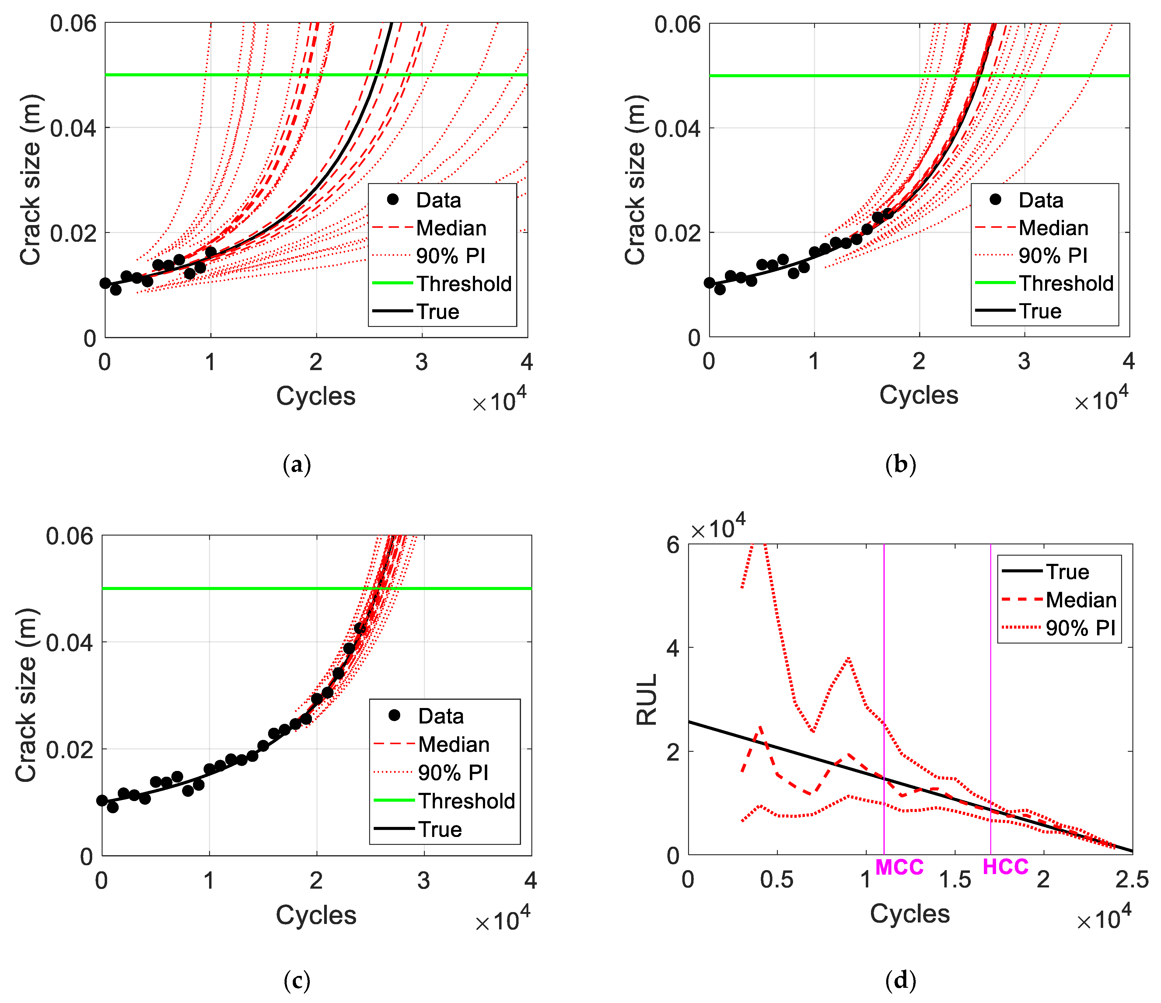
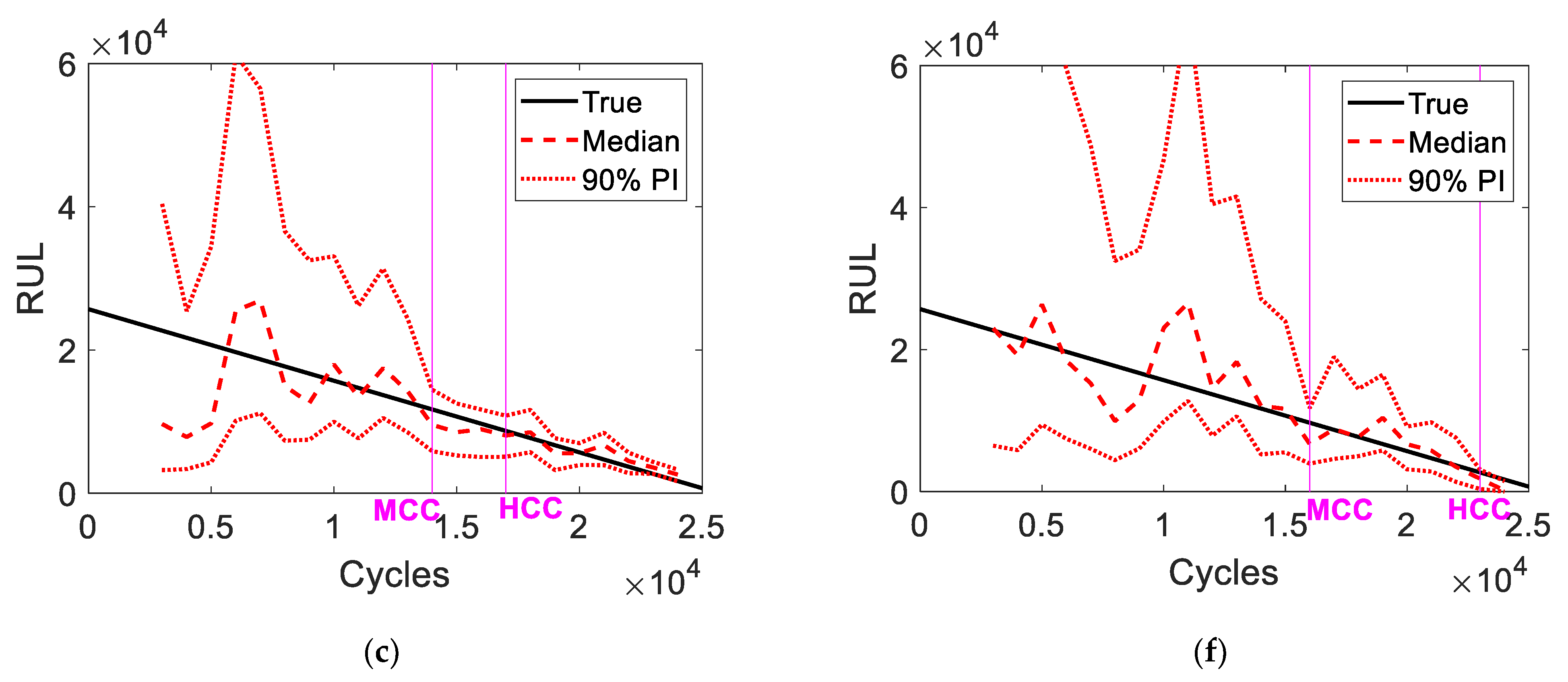
The results of the credibility criteria for the crack growth problem with a small level of noise are as shown in Figure 5b. It can be validated whether the criteria are reasonable by verifying the prediction results of damage growth and RUL according to the criteria zones. The damage prediction results for Zone 1 in Figure 5b are shown in Figure 6a together (red curves) with the true growth (black curve). It is shown that the PIs are too wide to make any decision, and thus the credibility of the prediction results is very low. However, the damage prediction results of Zone 2 in Figure 5b are properly distributed around the true growth, as shown in Figure 6b. This region provides a medium level of credibility, with moderate information to the level of noise in the data. 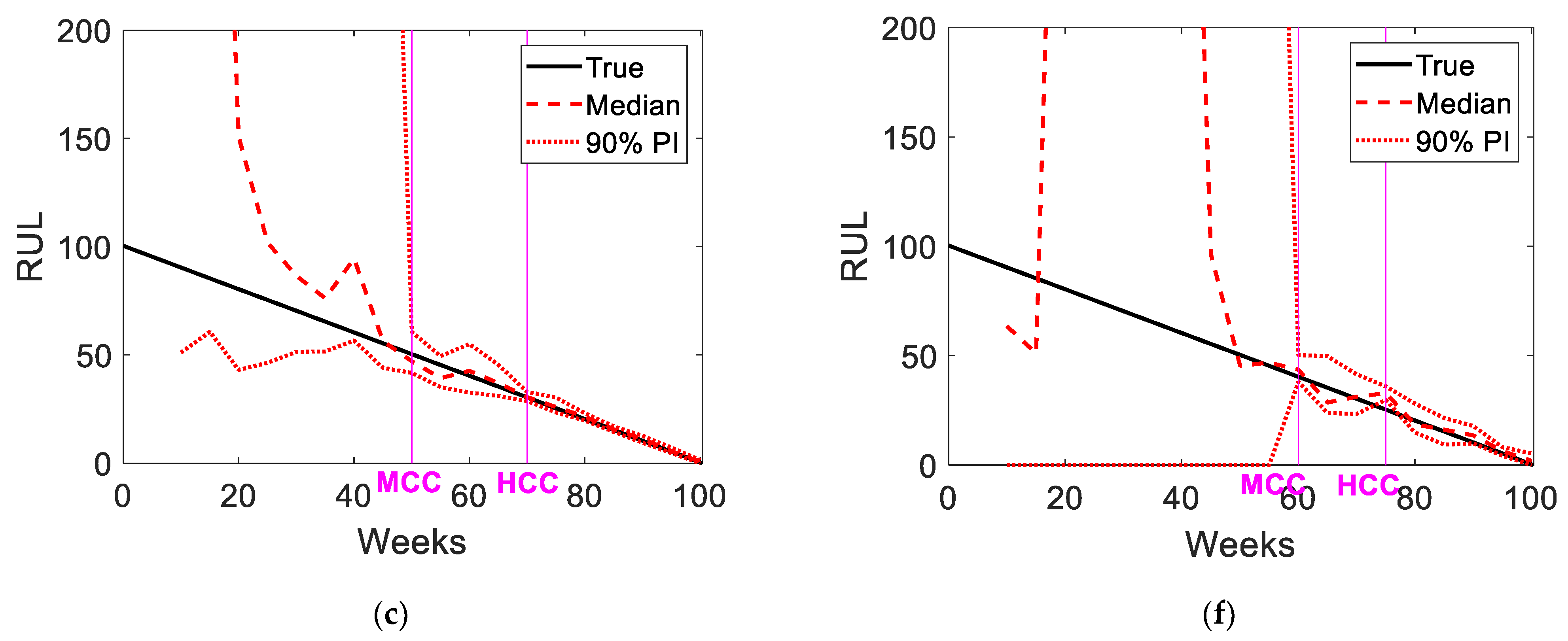The damage prediction results of Zone 3 in Figure 5b are shown in Figure 6c and are sufficiently updated because the prediction results are very close to the true growth of the medians and PIs. The RUL prediction results for the entire cycle are shown in Figure 6d. Figure 6 shows the same characteristic of the criteria zones mentioned in Section 3, and it is proven that the PI-based credibility criteria proposed in Section 3 are applicable. Note that there are no true values used to obtain Figure 5b.

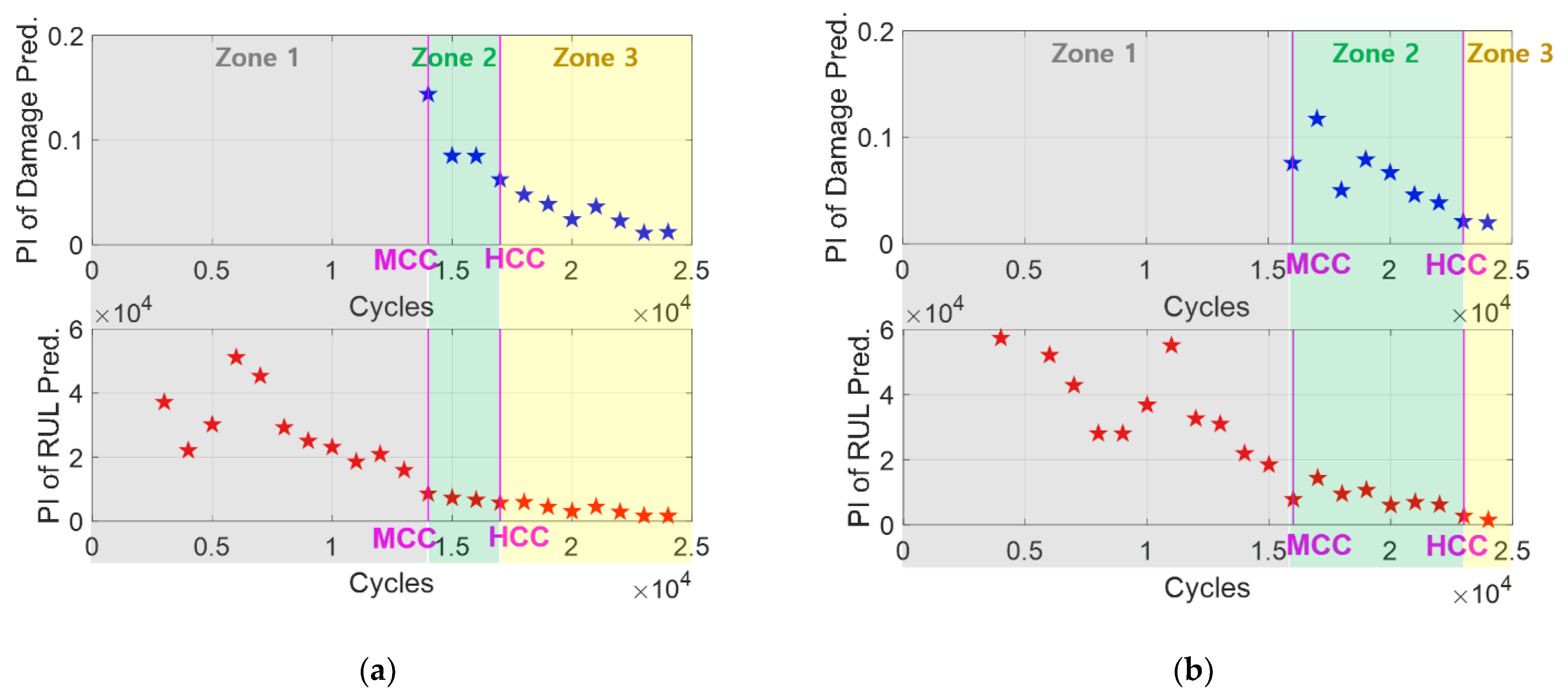
The results of the PI-based credibility criteria for two additional cases are shown in Figure 7. These cases have the same problem as the previous one, but they have a larger level of noise in the data than the previous one. Figure 7a,b show the results of the credibility criteria of medium and large levels of noise in the crack size, respectively, whose reasonability is shown in Figure 8. The damage prediction results in zones 2 and 3 of the medium level of noise are both feasible by properly distributing centering around the true growth, as shown in Figure 8a,b. By considering the level of noise in the data, the damage prediction results in Zone 3 are sufficiently updated because the PIs are not much wider than the noise level in the data. The RUL prediction results shown in Figure 8c also exhibit the same aspect. To validate the credibility criteria results shown in Figure 7b, the prediction results of the damage and RUL for the case of a large level of noise are shown in Figure 8d–f. Although the results of the damage prediction in zone 2 seem to have a large uncertainty from Figure 8d, it is still feasible to consider that level of noise in the data. It also makes sense that HCC is close to EOL under a large level of noise in the data, and thus, the prediction results of damage and RUL in zone 3 are not very informative, as shown in Figure 8e,f. Figure 8 shows that the results of the PI-based credibility criteria in Figure 7 are still applicable even under different levels of noise in the data, without any future information. Further discussion on the effect of noise on the criteria results is presented in Section 4.3.

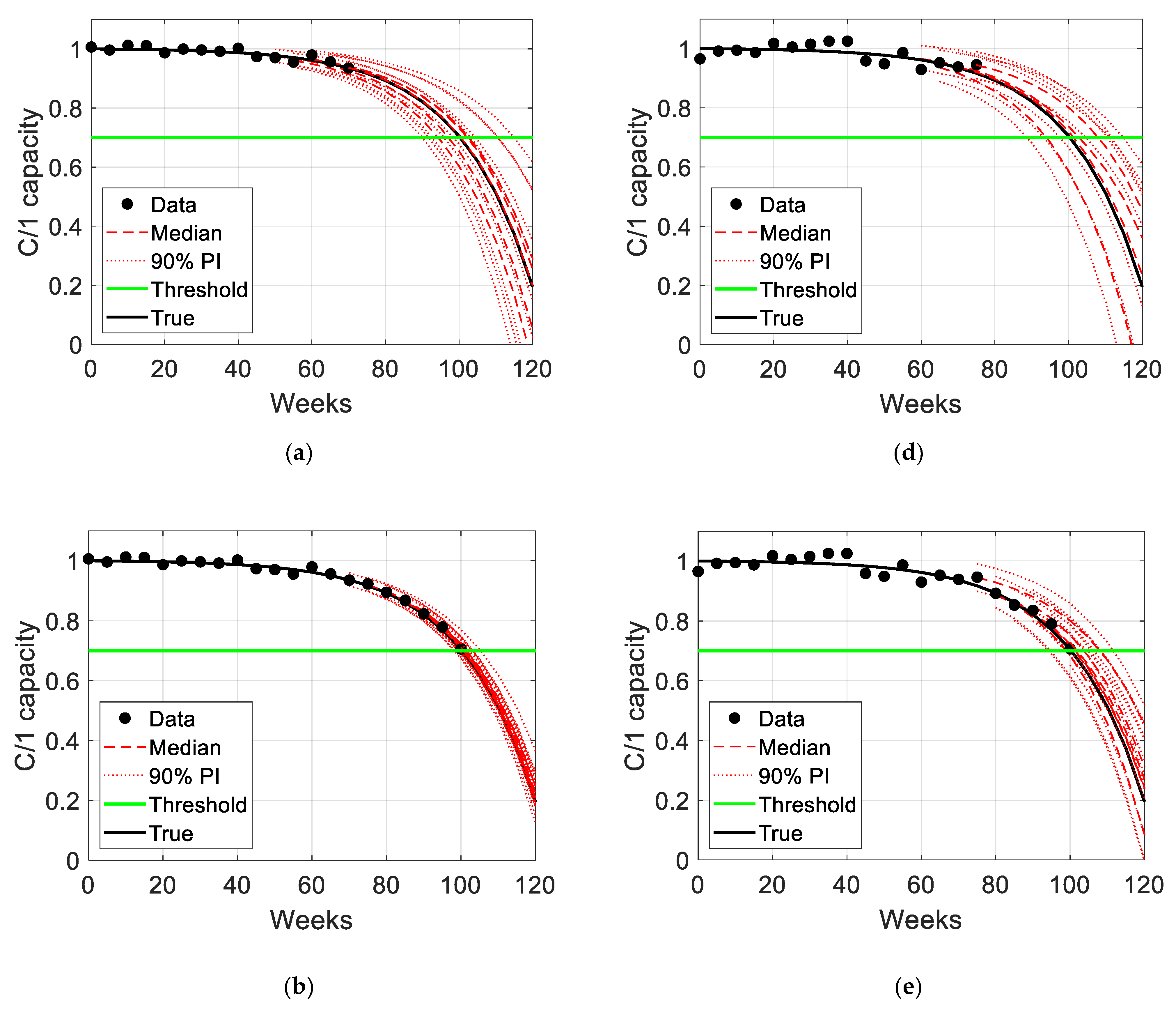
4.2. Battery Degradation Problem

The capacity of a secondary cell, such as a lithium-ion battery, degrades with the number of cycles used, and the degradation performance is represented by the C/1 capacity, which is the capacity at a nominally rated current of 1A [18]. It is assumed that a battery is in use under fully charging–discharging conditions, and the degradation behavior is usually expressed by an exponential function, such as

$$y_k=\left(y_{k-1}-b\right)\exp \left(\frac{\Delta t}{20}\right)+b,\Delta t=t_k-t_{k-1},$$

(5)

where y is the C/1 capacity, k is the current time index, and b is the model parameter to be estimated.

It is assumed that the C/1 capacity is measured every 5 weeks (i.e., $\Delta t=5$), and the threshold is defined when the capacity fades by 30% of the initial condition, i.e., the threshold is 0.7 for the C/1 capacity. The last piece of information required for the prognostics process is that of the capacity for each measurement cycle. Battery capacity data are also generated synthetically by assuming the true values of model parameters as b_true = 1.002, which are only used for data generation and are practically unknown during the prognostics process. In the battery problem, the PI-based credibility criteria are validated with two different levels of noise: small and medium.

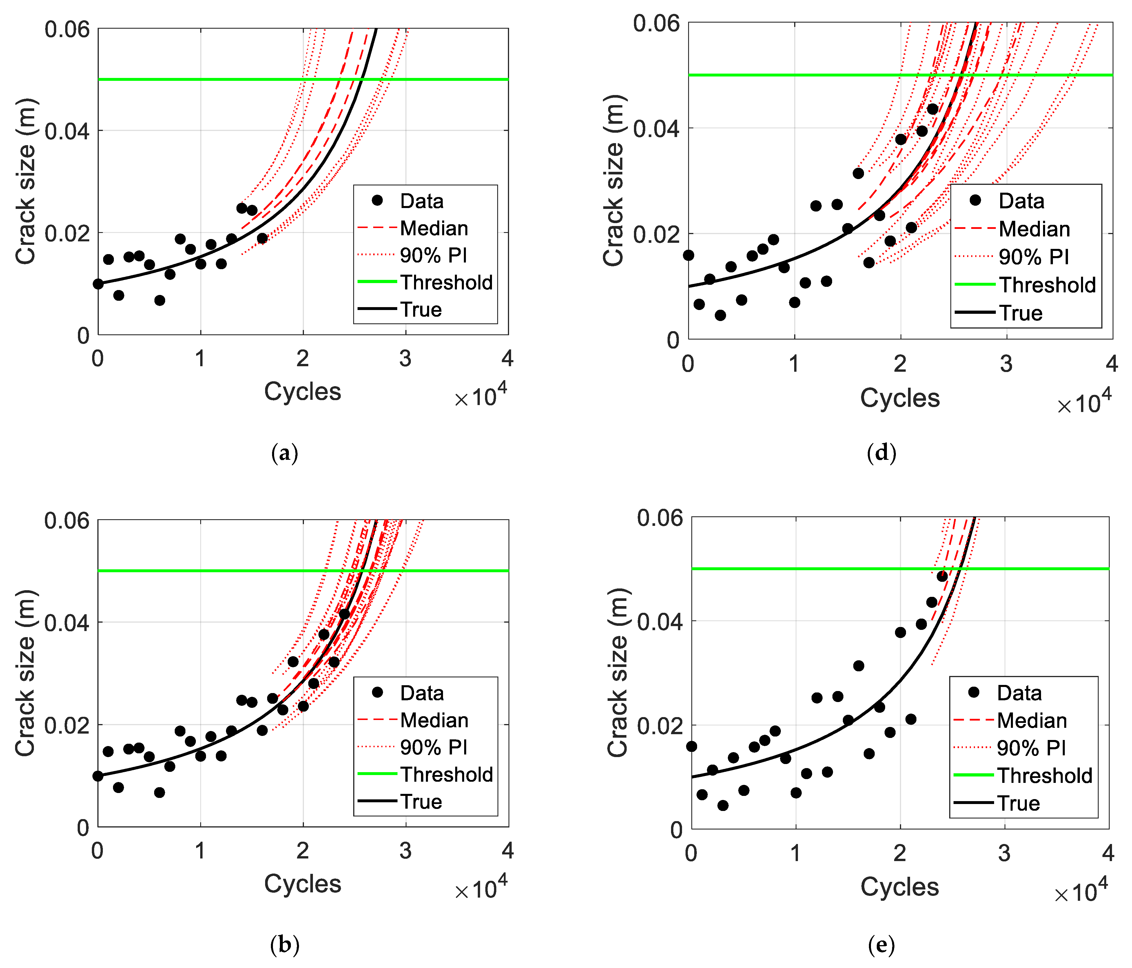
The results of the PI-based credibility criteria are shown in Figure 9, followed by the validation in Figure 10. For the case of small level of noise in Figure 9a, the credibility criteria results represent that the prognostics results are feasible after 50 weeks (MCC), and then they become fairly reliable after 70 weeks (HCC) with sufficient data related to the level of noise. The reasonability of the criteria results is shown in Figure 10a–c. The damage prediction results in zones 2 and 3 with a small level of noise are both feasible by properly distributing centering around the true growth, as shown in Figure 10a,b. In addition, it is shown that the damage prediction results in Zone 3 are sufficiently updated under the given conditions, and there is mostly inherent noise in the data, as shown in Figure 10b. The RUL prediction results in Figure 10c also show the same aspect as the prediction of the degradation behavior. For the case of a medium level of noise in Figure 9b, MCC and HCC are 60 and 75 weeks, respectively. The reasonability of the criteria results is shown in Figure 10d–f by showing that the prediction results of damage and RUL after MCC are feasible, and the prediction results are sufficiently updated after HCC under the given conditions.

4.3. Discussions

The PI-based credibility criteria proposed in this article are simple, intuitive, and practical because practical digits are expressed with two graphical results, as shown in Figure 5b, Figure 7 and Figure 9. In particular, MCC is very clear because it is a kind of all-or-nothing decision. However, HCC can differ according to how it is defined. For example, the definition of HCC in this article is the first cycle when the PIs of both damage and RUL simultaneously decrease ‘three’ continuous times, but it also could be ‘four’ continuous times. Even though the ‘three’ times is not an absolute standard, it could be a general standard. The reasonability of the definitions of MCC and HCC is discussed based on the results from the five case studies in Figure 5b, Figure 7 and Figure 9.

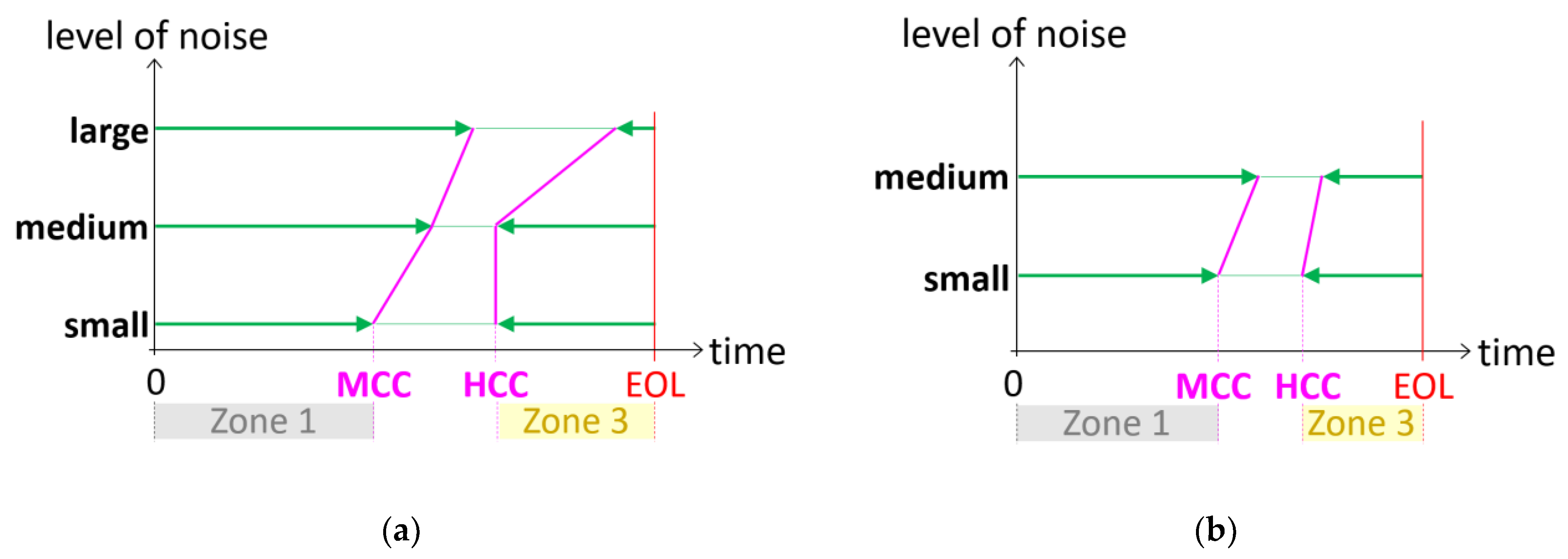
The MCC and HCC results for the five cases are shown in Figure 11. MCC and HCC are depicted according to their proportions as green arrows. For the crack growth problem in Figure 11a, as the level of noise increases, MCC starts late, and HCC comes close to EOL. This is a reasonable phenomenon, and the same tendency is observed in the battery example, as shown in Figure 11b. Therefore, the PI-based credibility criteria can be used to make a decision on the prognostics results in practice without the true values of degradation behavior and RUL.

5. Conclusions

Prognostics results are obtained with a distribution to cover uncertainties caused by several sources, such as quality and quantity in the data and prediction processes. Although it is common sense that uncertainty is present everywhere, the performance evaluation is focused on the accuracy of the results. This research custom allows us to compare the prediction result with the true value, which is impractical. Although the true value-based evaluation approach is still useful and necessary to validate new methods, it does not pertain to the industry at all. Therefore, this article presents the credibility criteria of prognostics results based on the PI; five cases from two different problems are used for the validation. According to the credibility criteria, the prognostics results are feasible after MCC, which is the first cycle when reasonable values are shown for both the damage and RUL PIs. In addition, the prognostics results are feasible with high credibility after HCC, which is the first cycle when the PIs of both damage and RUL simultaneously decrease three continuous times after MCC. Consequently, the proposed credibility criteria are simple, intuitive, and practical because they are expressed with two graphical results, using practical digits (PIs) obtained at every measurement cycle.