
Process Hazard Analysis Based on Modeling and Simulation Tools


Abstract
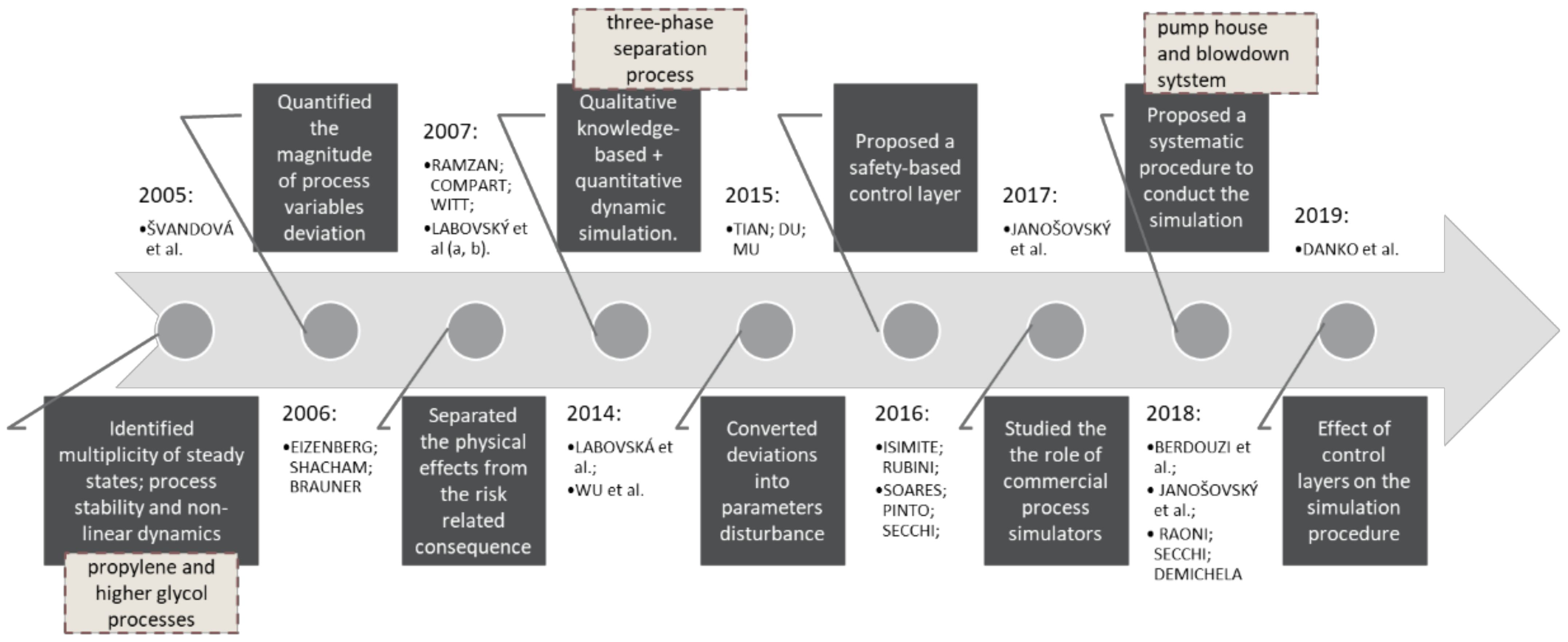
:1. Introduction
2. Methods and Case-Study
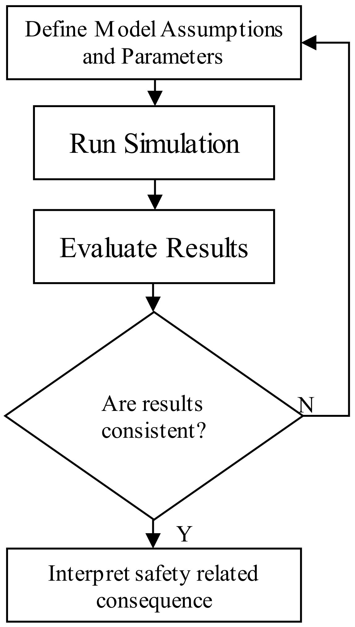
2.1. Proposal of a Hazard Identification Method
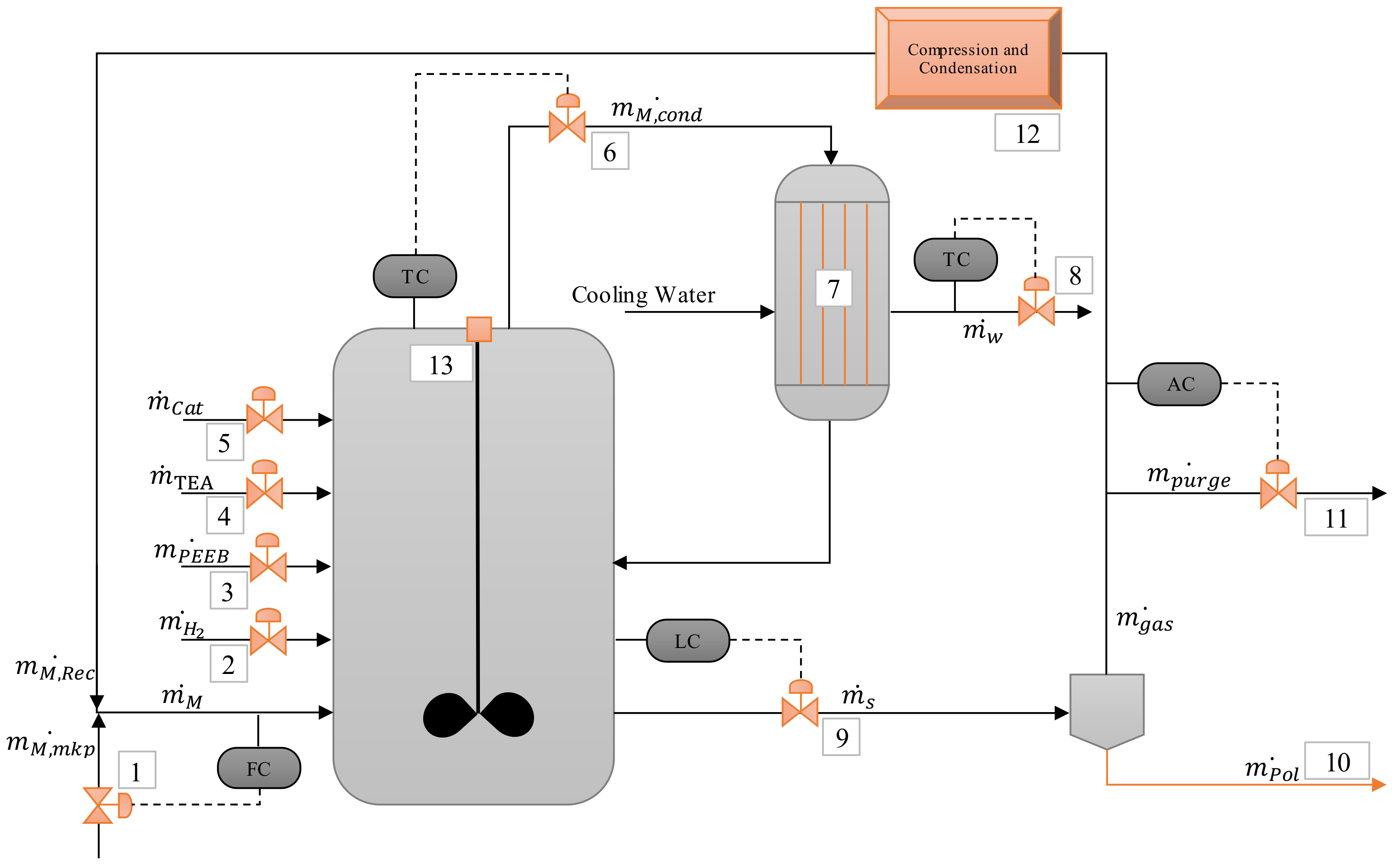
2.2. Case Study: Bulk Polymerization of Propene
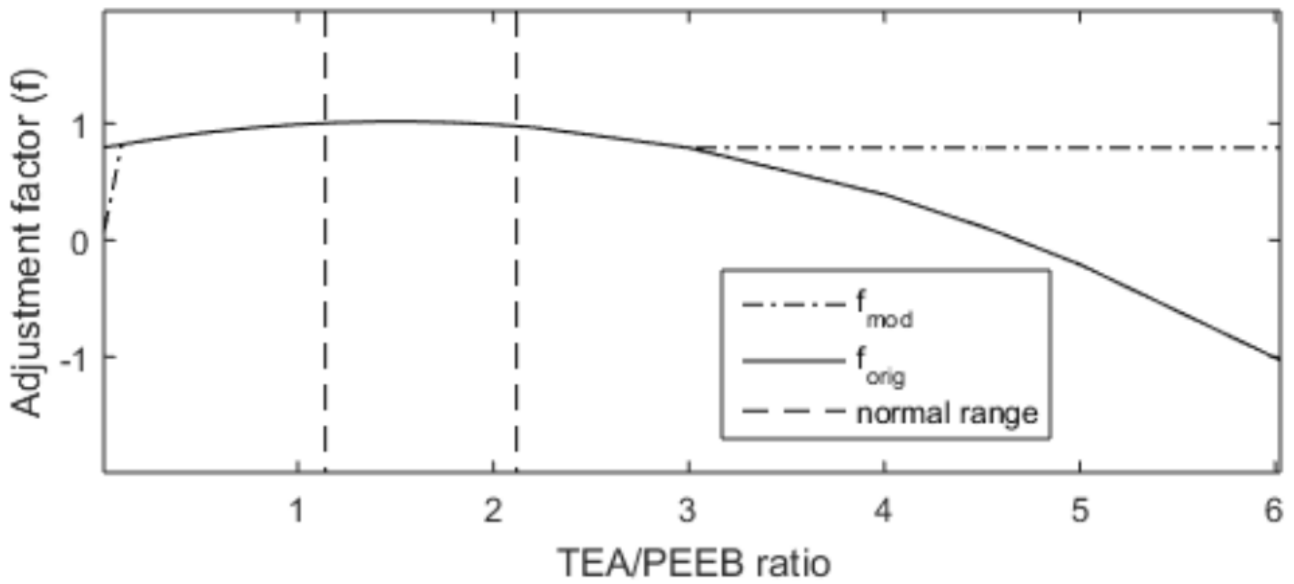
2.2.1. Model Adaptation
- introduce a linear approximation up to zero in the region of low TEA concentrations, since it is known that TEA (co-catalyst) is needed to activate the catalyst [22];
- assume a constant behavior of 80% of deactivation in the region of low PEEB concentrations, since it is known that the excess of PEEB jeopardizes mainly the quality of the final product and is not able to kill the reaction [23].
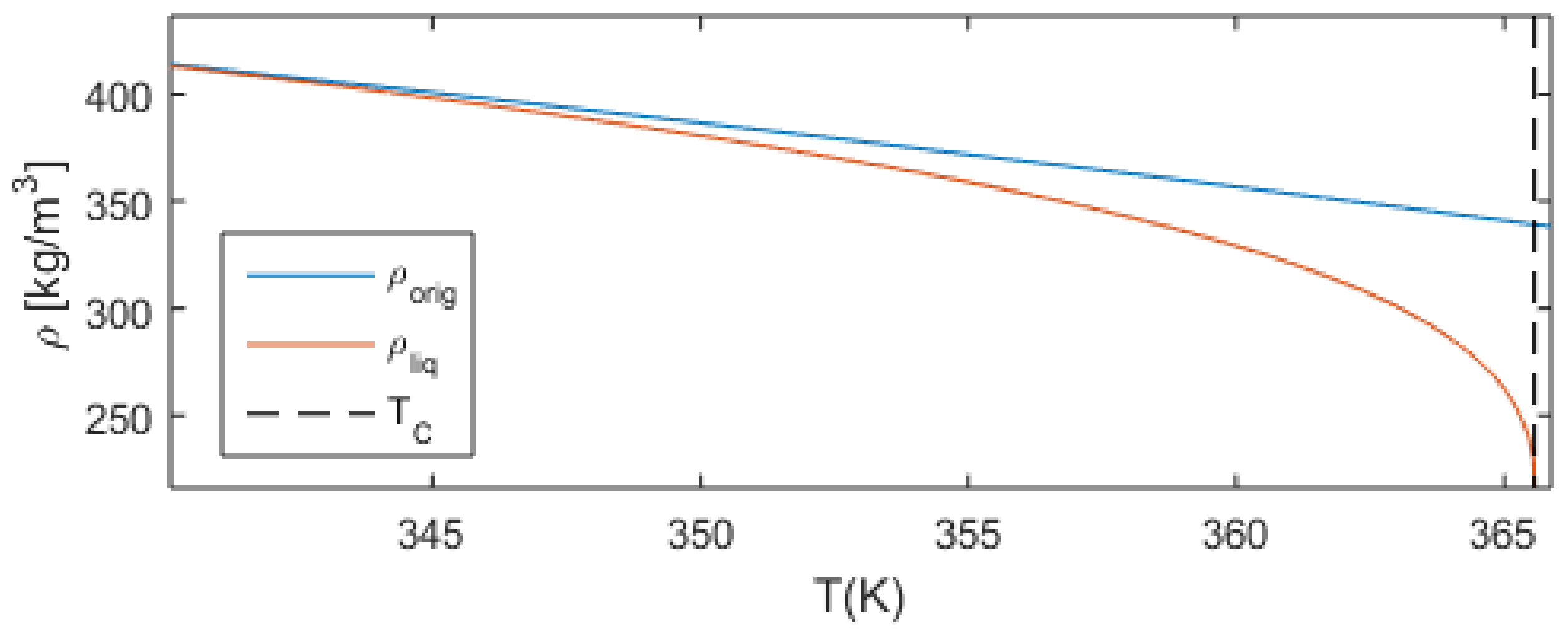
- subcooled liquid is assumed if ;
- overheated vapor is assumed if ;
- and liquid-vapor phase equilibrium is assumed if .
3. Results
3.1. Device Malfunction Identification
3.2. Simulations
- Volume (V): the normal operation condition represents 60% of the design limit of .
- Pressure (P): the normal operation condition represents 60% of the maximum allowed working pressure (MAWP) of .
- Temperature (T): the normal operation condition is approximately 50 K below the design temperature of 400 K.
3.3. Malfunction Simulations
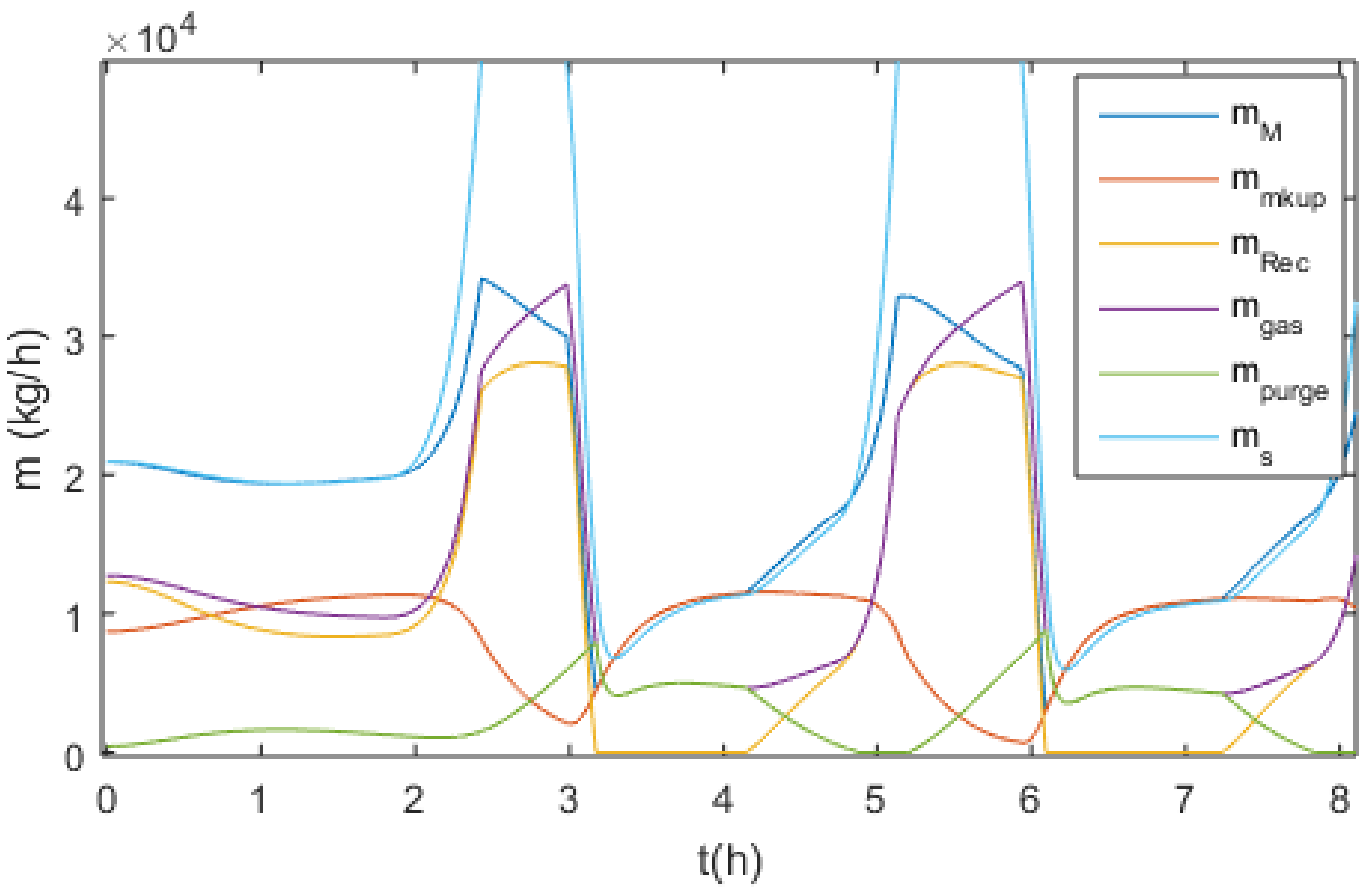
3.3.1. S-1 (No Monomer Make-Up Flowrate) and S-2 (Lower Monomer Make-Up Flowrate)
3.3.2. S-3 (Higher Monomer Make-Up Flowrate)
3.3.3. S-10 and S-11 (No and Lower PEEB Feed Flowrate)
3.3.4. S-13 and S-14 (No and Lower TEA Feed Flowrate)
3.3.5. S-18 (Higher Catalyst Feed Flowrate)
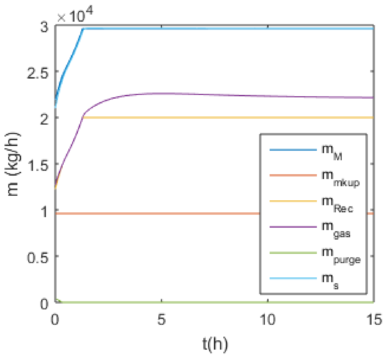
3.3.6. S-29 and S-30 (No and Lower Outlet Slurry Mass Flowrate)
3.3.7. S-35 (Higher Recycled Monomer Purge Flowrate)
4. Discussion
4.1. Safety Considerations after Simulation Results
4.2. Comparison with Traditional HAZOP
- Both HAZOP teams had the perception of being unconservative or conservative when they, in fact, were (comparing with the simulation results) and would recommend process simulations to check their understandings. In the cases of significant different results, in 60% of the cases, the HAZOP team was not confident and recommended the simulation.
- In some cases, the inclusion of a flow model with pressure drop and pressure propagation would be helpful to support understanding of the final consequences.
- The HAZOP team’s creativeness allowed for the identification of mid- and long-term effects after the failure occurrence. In addition, possible effects regarding start-up after the failure condition were discussed. This introduces a relevant aspect that should have been added to the computational-based methodology: simulate a malfunction step and, from the malfunction condition, simulate a step back to the normal value.
5. Conclusions
- Risk assessment for each scenario and the design of safety barriers, since the present hazard identification study alerted for different hazard situations, mainly related to the hydrodynamic collapse of the reaction suspension, that must be prevented and mitigated;
- Design of a safety-based control layer, since the present hazard study identified different device failures leading to the undesired hydrodynamic collapse of the reaction suspension, which poses a significant risk of process shutdown [23];
- Proposal of online model-based risk in order to indicate the evolution of the process safety and allow for predictive maintenance and effective decision-making that can minimize costs and prevent accidents and losses.
Author Contributions
Funding
Institutional Review Board Statement
Informed Consent Statement
Data Availability Statement
Conflicts of Interest
References
- Bowonder, B. The Bhopal accident. Technol. Forecast. Soc. Change 1987, 32, 169–182. [Google Scholar] [CrossRef]
- Gordon, R.P.E. The contribution of human factors to accidents in the offshore oil industry. Reliab. Eng. Syst. Saf. 1998, 61, 95–108. [Google Scholar] [CrossRef]
- Venart, J.E.S. Flixborough: The explosion and its aftermath. Process Saf. Environ. Prot. 2004, 82, 105–127. [Google Scholar] [CrossRef]
- Pasman, H. Risk Analysis and Control for Industrial Processes Gas, Oil and Chemicals; Butterworth Heinemann: Waltham, MA, USA, 2015. [Google Scholar]
- Center for Chemical Process Safety. Guidelines for Hazard Evaluation Procedures, 2nd ed.; American Institute of Chemical Engineers, Ed.; American Institute of Chemical Engineers: New York, NY, USA, 1992. [Google Scholar]
- Papazoglou, I.; Aneziris, O. Master Logic Diagram: Method for hazard and initiating event identification in process plants. J. Hazard. Mater. 2003, 97, 11–30. [Google Scholar] [CrossRef]
- Crowl, D.; Louvar, J. Chemical Process Safety: Fundamentals with Applicattions, 2nd ed.; Prentice Hall PTR: Upper Saddle River, NJ, USA, 2002. [Google Scholar]
- Graf, H.; Schmidt-Traub, H. Early hazard identification of chemical plants with statechart modelling techniques. Saf. Sci. 2000, 36, 49–67. [Google Scholar] [CrossRef]
- Dunjó, J.; Fthenakis, V.; Vílchez, J.A.; Arnaldos, J. Hazard and operability (HAZOP) analysis. A literature review. J. Hazard. Mater. 2010, 173, 19–32. [Google Scholar] [CrossRef]
- Graf, H.; Schmidt-Traub, H. Process hazard identification during plant design by qualitative modelling, simulation and analysis. Comput. Chem. Eng. 1999, 23, S59–S62. [Google Scholar] [CrossRef]
- Tian, W.; Du, T.; Mu, S. HAZOP analysis-based dynamic simulation and its application in chemical processes. Asia-Pac. J. Chem. Eng. 2015, 10, 923–935. [Google Scholar] [CrossRef]
- Švandová, Z.; Jelemenský, L.; Markoš, J.; Molnár, A. Steady States Analysis and Dynamic Simulation as a Complement in the Hazop Study of Chemical Reactors. Process Saf. Environ. Prot. 2005, 83, 463–471. [Google Scholar] [CrossRef]
- Venkatasubramanian, V.; Vaidhyanathan, R. A knowledge-based framework for automating HAZOP analysis. AIChE J. 1994, 40, 496–505. [Google Scholar] [CrossRef]
- Labovská, Z.; Labovský, J.; Jelemenský, Ľ.; Dudáš, J.; Markoš, J. Model-based hazard identification in multiphase chemical reactors. J. Loss Prev. Process Ind. 2014, 29, 155–162. [Google Scholar] [CrossRef]
- Baybutt, P. A critique of the Hazard and Operability (HAZOP) study. J. Loss Prev. Process Ind. 2015, 33, 52–58. [Google Scholar] [CrossRef]
- Raoni, R.; Secchi, A.R.; Demichela, M. Employing process simulation for hazardous process deviation identification and analysis. Saf. Sci. 2018, 101, 209–219. [Google Scholar] [CrossRef]
- Mattos Neto, A.G.; Pinto, J.C. Steady-state modeling of slurry and bulk propylene polymerizations. Chem. Eng. Sci. 2001, 56, 4043–4057. [Google Scholar] [CrossRef]
- Prata, D.M.; Schwaab, M.; Lima, E.L.; Pinto, J.C. Nonlinear dynamic data reconciliation and parameter estimation through particle swarm optimization: Application for an industrial polypropylene reactor. Chem. Eng. Sci. J. 2009, 64, 21–22. [Google Scholar] [CrossRef]
- Dutra, J.C.S.; de Feital, T.S.; Skogestad, S.; Lima, E.L.; Pinto, J.C. Control of Bulk Propylene Polymerizations Operated with Multiple Catalysts through Controller Reconfiguration. Macromol. React. Eng. 2014, 8, 201–216. [Google Scholar] [CrossRef]
- Dos Santos Silva, J. Otimizacão da Transição de Grades na Polimerizacão em Massa do Propeno. Ph.D. Thesis, Universidade Federal do Rio de Janeiro, COPPE, Rio de Janeiro, Brazil, 2018. [Google Scholar]
- Coimbra, J.C.; Melo, P.A.; Prata, D.M.; Pinto, J.C. On-line dynamic data reconciliation in batch suspension polymerizations of methyl methacrylate. Processes 2017, 5, 51. [Google Scholar] [CrossRef]
- Malpass, D.B.; Band, E.I. Introduction to Industrial Polypropylene; Scrivener Publishing: Beverly, MA, USA, 2012; ISBN 9781118062760. [Google Scholar]
- Soares, R.M.; Pinto, J.C.; Secchi, A.R. An optimal control-based safety system for cost efficient risk management of chemical processes. Comput. Chem. Eng. 2016, 91, 471–484. [Google Scholar] [CrossRef]
- Angus, S.; Armstrong, B.; De Reuck, K.M. Propylene (Propene)-International Thermodynamic Tables of the Fluid State; Pergamon Press: Oxford, UK, 1980; Volume 7. [Google Scholar]
- NIST Reference Fluid Thermodynamic and Transport Properties Database (REFPROP Version 7). Available online: https://webbook.nist.gov/cgi/fluid.cgi?ID=C115071&Action=Page (accessed on 24 June 2019).
- Neduzhii, I.A.; Vashchenko, D.M.; Voinov, Y.F.; Voityuk, B.V.; Dregulyas, E.K.; Kolomiets, A.Y.; Labinov, S.D.; Morozov, A.A.; Provotar, V.P.; Soldatenko, Y.A.; et al. Thermodynamic and Transport Properties of Ethylene and Propylene; National Bureau of Standards Department of Commerce: Washington, DC, USA, 1972; ISBN 978-0-631-19703-4.
- Rebillot, P.F.; Jacobs, D.T. Heat capacity anomaly near the critical point of aniline-cyclohexane. J. Chem. Phys. 1998, 109, 4009–4014. [Google Scholar] [CrossRef]
- Nowicki, A.W.; Ghosh, M.; McClellan, S.M.; Jacobs, D.T. Heat capacity and turbidity near the critical point of succinonitrile-water. J. Chem. Phys. 2001, 114, 4625–4633. [Google Scholar] [CrossRef]
- Prata, D.M. Reconciliação Robusta de Dados para Monitoramento em Tempo Real. Ph.D. Thesis, Universidade Federal do Rio de Janeiro: COPPE, Rio de Janeiro, Brazil, 2009. [Google Scholar]
- Da Silva Rosa, I.; Melo, P.A.; Pinto, J.C. Bifurcation analysis of the bulk propylene polymerization in the LIPP process. Macromol. Symp. 2012, 319, 41–47. [Google Scholar] [CrossRef]
- Oliveira, A.G.; Candreva, P.M.; Melo, P.A.; Pinto, J.C. Steady-state behavior of slurry and bulk propylene polymerization. Polym. React. Eng. 2006, 11, 155–176. [Google Scholar] [CrossRef]
- Labovský, J.; Švandová, Z.; Markoš, J.; Jelemenský, L. Model-based HAZOP study of a real MTBE plant. J. Loss Prev. Process Ind. 2007, 20, 230–237. [Google Scholar] [CrossRef]


 ) no flow; (
  ) of normal flow; (
  ) of normal flow; (
  ) of normal flow; (
  ) normal.
) no flow; ( ) of normal flow; ( ) of normal flow; ( ) of normal flow; ( ) normal.
) normal.
) no flow; ( ) of normal flow; ( ) of normal flow; ( ) of normal flow; ( ) normal.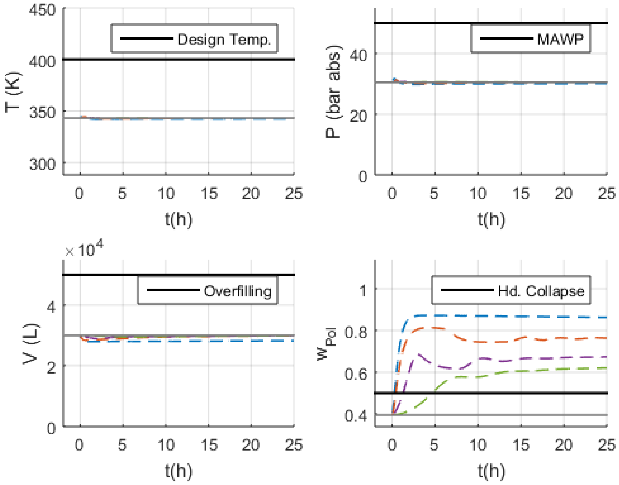
 ) no flow; (
  ) of normal flow; (
  ) of normal flow; (
  ) of normal flow; (
  ) normal.
) no flow; ( ) of normal flow; ( ) of normal flow; ( ) of normal flow; ( ) normal.
) normal.
) no flow; ( ) of normal flow; ( ) of normal flow; ( ) of normal flow; ( ) normal.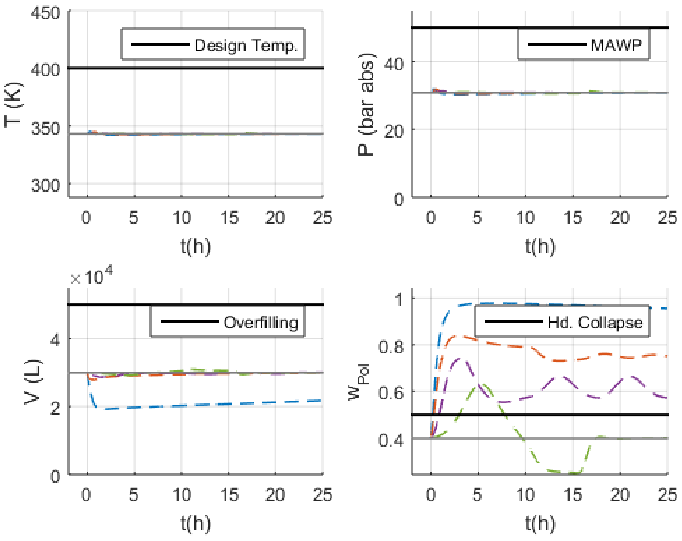
 ) no flow; (
  ) of normal flow; (
  ) of normal flow; (
  ) of normal flow; (
  ) normal.
) no flow; ( ) of normal flow; ( ) of normal flow; ( ) of normal flow; ( ) normal.
) normal.
) no flow; ( ) of normal flow; ( ) of normal flow; ( ) of normal flow; ( ) normal.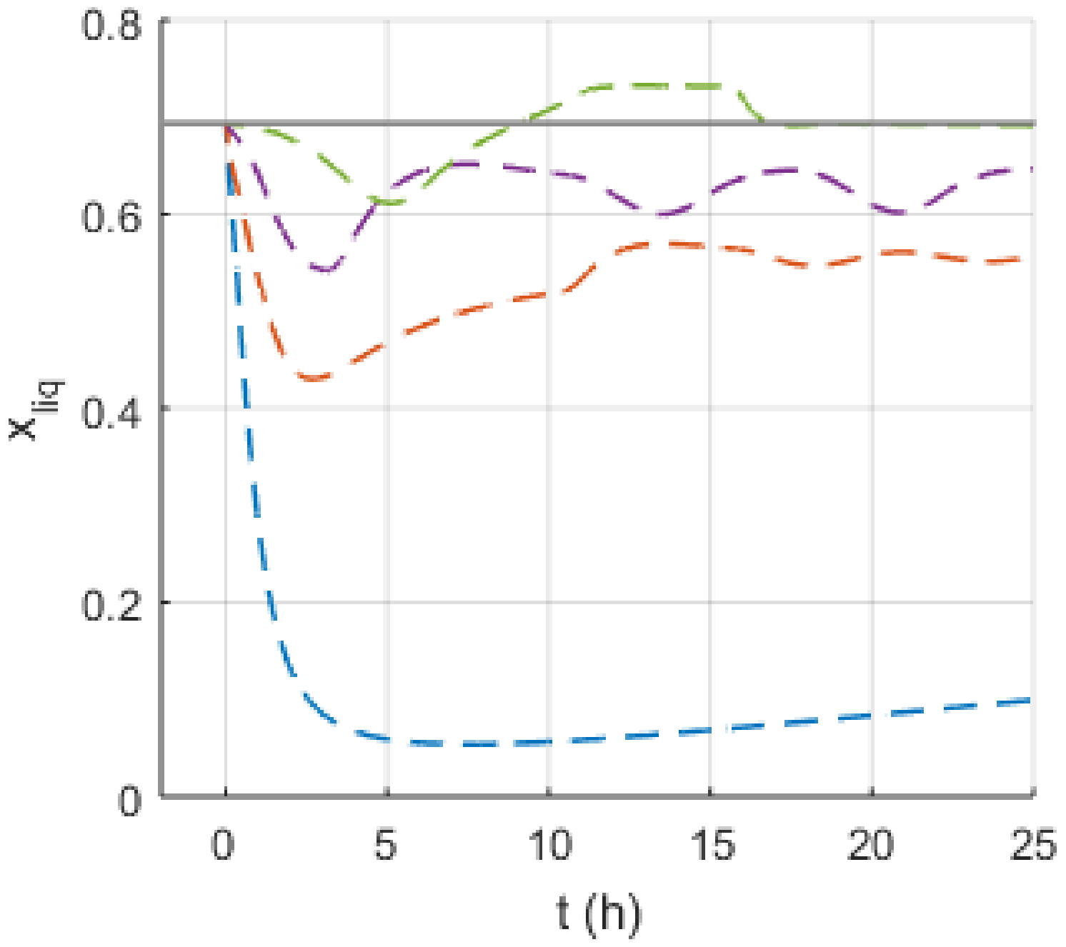
 ) maximum flow; (
  ) of normal flow; (
  ) of normal flow; (
  ) of normal flow; (
  ) normal.
) maximum flow; ( ) of normal flow; ( ) of normal flow; ( ) of normal flow; ( ) normal.
) normal.
) maximum flow; ( ) of normal flow; ( ) of normal flow; ( ) of normal flow; ( ) normal.
 ) maximum flow; (
  ) of normal flow; (
  ) of normal flow; (
  ) of normal flow; (
  ) normal.
) maximum flow; ( ) of normal flow; ( ) of normal flow; ( ) of normal flow; ( ) normal.
) normal.
) maximum flow; ( ) of normal flow; ( ) of normal flow; ( ) of normal flow; ( ) normal.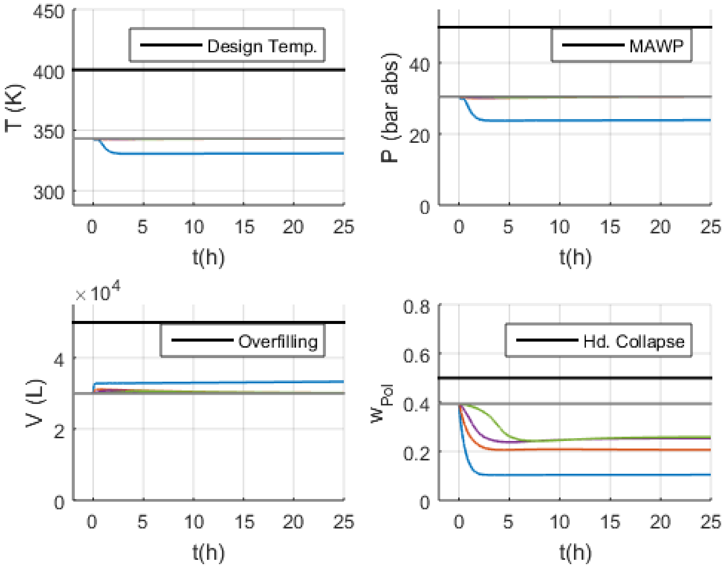
 ) no flow; (
  ) of normal flow; (
  ) of normal flow; (
  ) of normal flow; (
  ) normal.
) no flow; ( ) of normal flow; ( ) of normal flow; ( ) of normal flow; ( ) normal.
) normal.
) no flow; ( ) of normal flow; ( ) of normal flow; ( ) of normal flow; ( ) normal.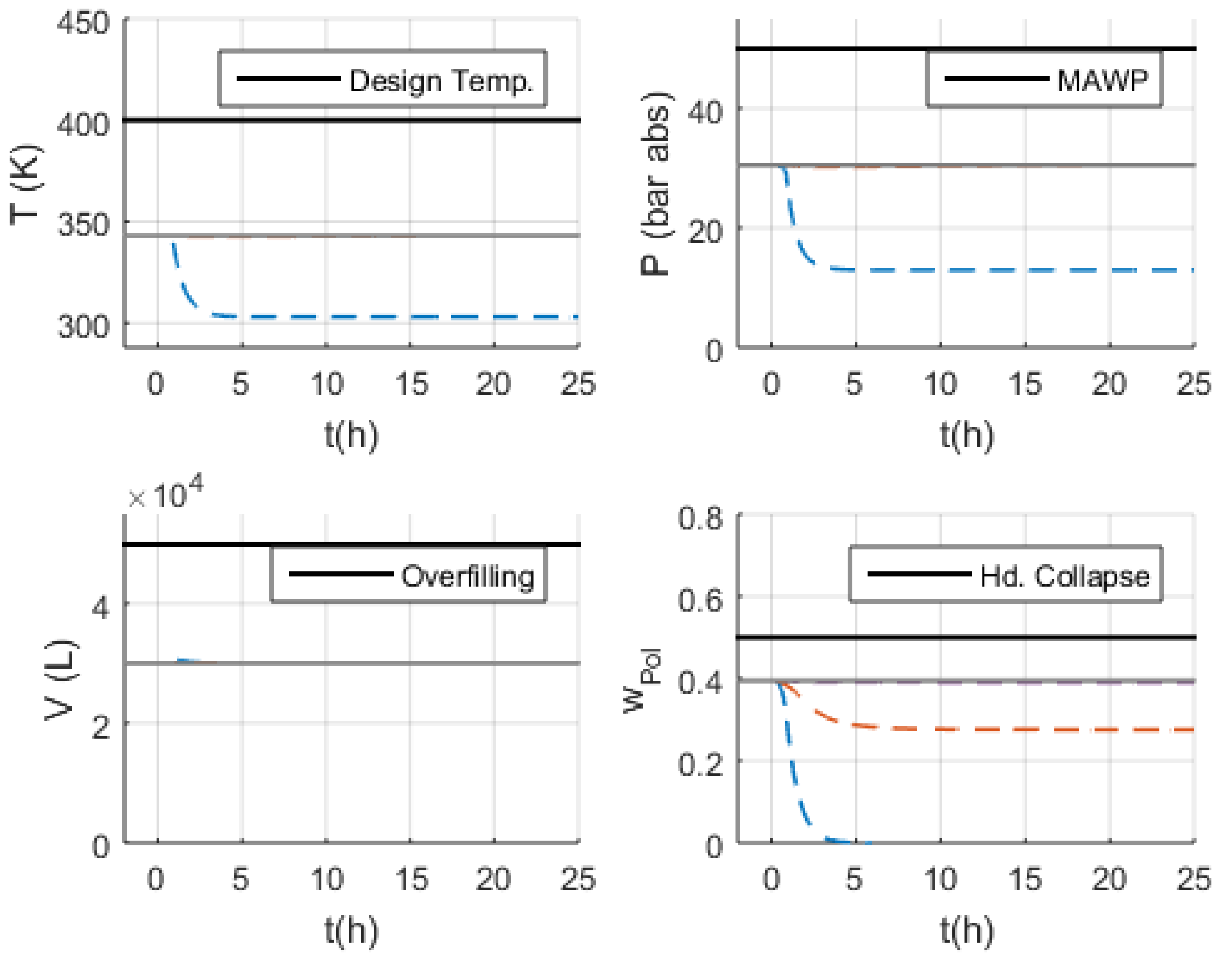
 ) no flow; (
  ) of normal flow; (
  ) of normal flow; (
  ) of normal flow; (
  ) normal.
) no flow; ( ) of normal flow; ( ) of normal flow; ( ) of normal flow; ( ) normal.
) normal.
) no flow; ( ) of normal flow; ( ) of normal flow; ( ) of normal flow; ( ) normal.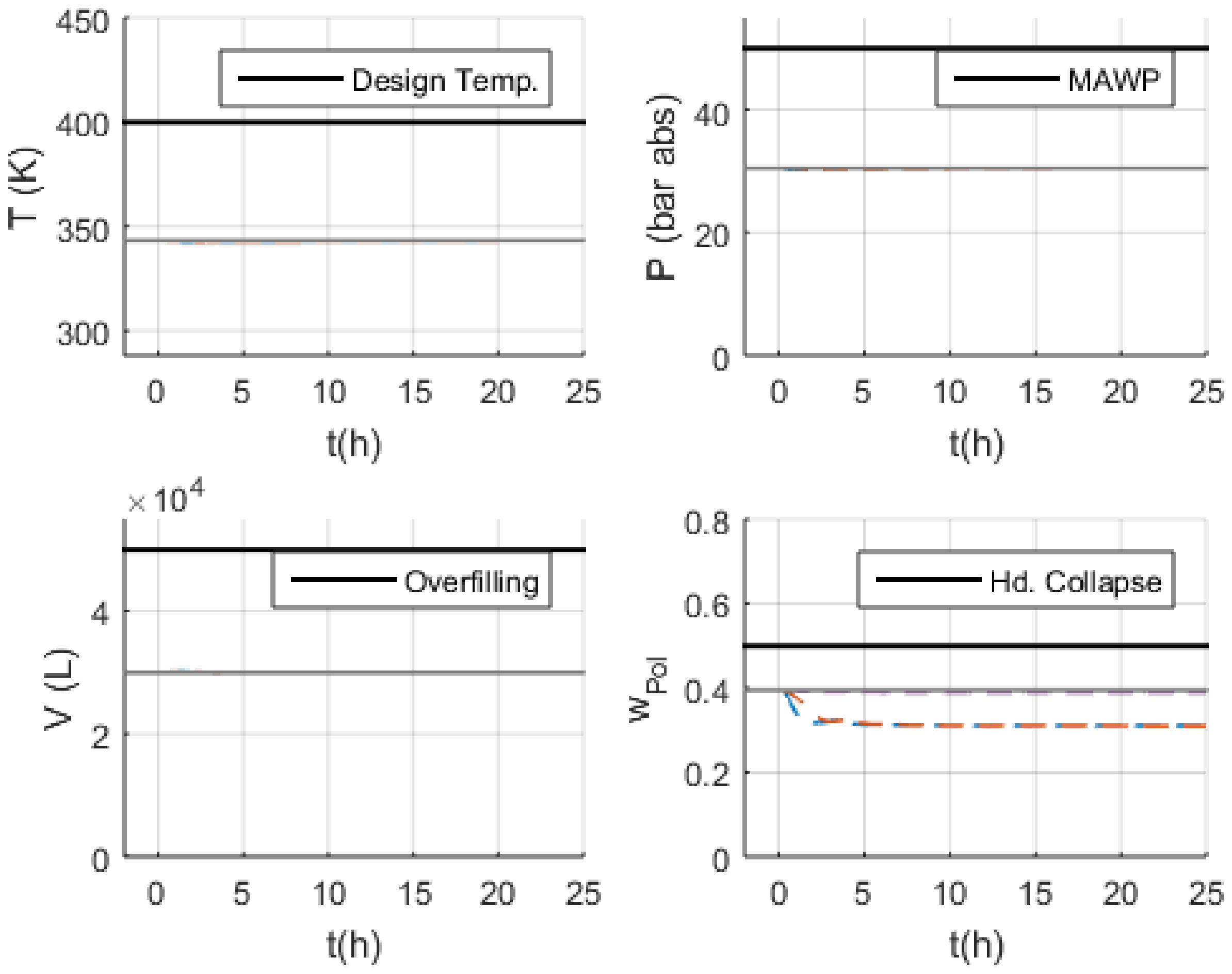
 ) no flow; (
  ) of normal flow; (
  ) of normal flow; (
  ) of normal flow; (
  ) normal.
) no flow; ( ) of normal flow; ( ) of normal flow; ( ) of normal flow; ( ) normal.
) normal.
) no flow; ( ) of normal flow; ( ) of normal flow; ( ) of normal flow; ( ) normal.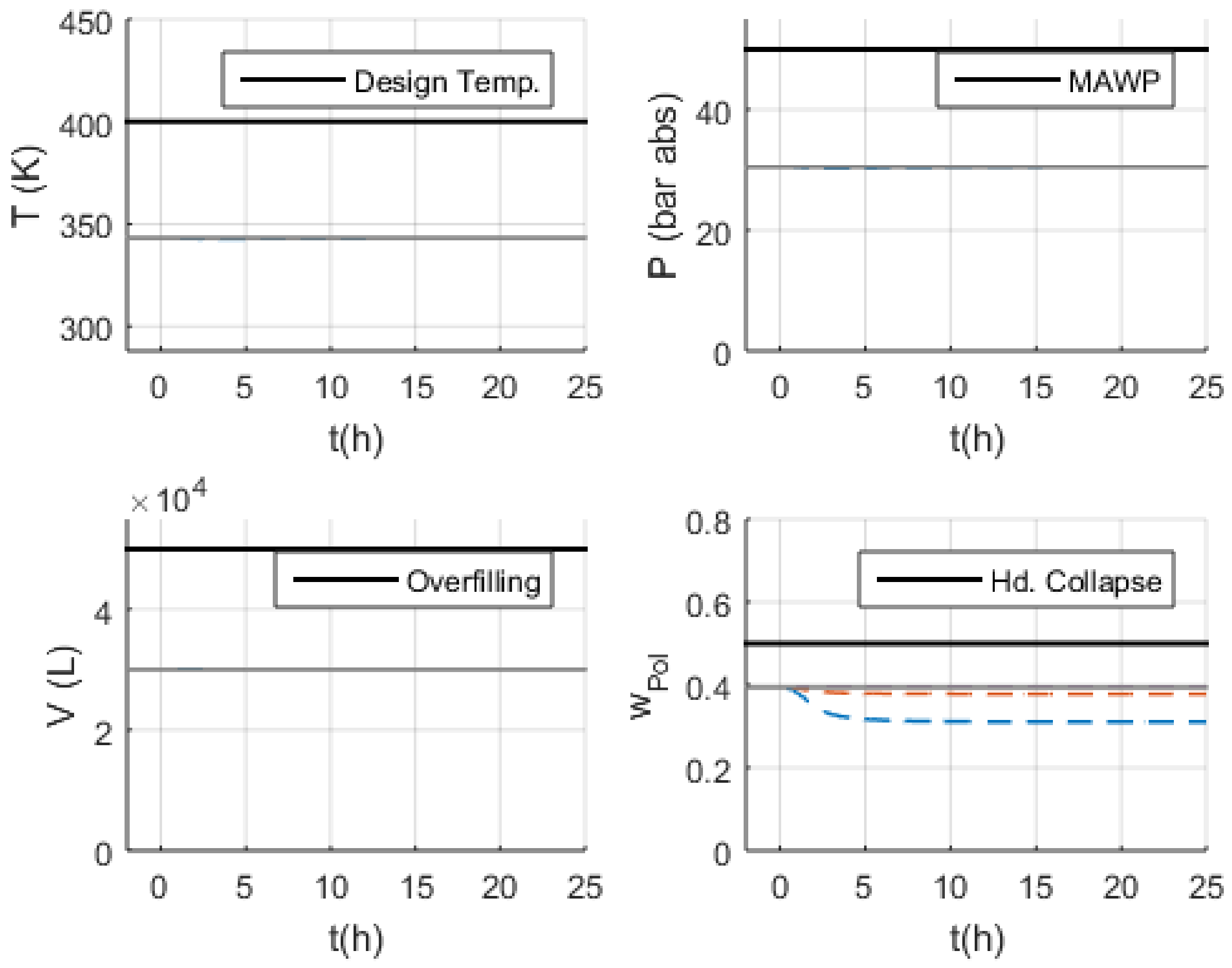
 ) no flow; (
  ) of normal flow; (
  ) of normal flow; (
  ) of normal flow; (
  ) normal.
) no flow; ( ) of normal flow; ( ) of normal flow; ( ) of normal flow; ( ) normal.
) normal.
) no flow; ( ) of normal flow; ( ) of normal flow; ( ) of normal flow; ( ) normal.
 ) maximum flow; (
  ) of normal flow; (
  ) of normal flow; (
  ) of normal flow; (
  ) normal.
) maximum flow; ( ) of normal flow; ( ) of normal flow; ( ) of normal flow; ( ) normal.
) normal.
) maximum flow; ( ) of normal flow; ( ) of normal flow; ( ) of normal flow; ( ) normal.
 ) maximum flow; (
  ) of normal flow; (
  ) of normal flow; (
  ) of normal flow; (
  ) normal.
) maximum flow; ( ) of normal flow; ( ) of normal flow; ( ) of normal flow; ( ) normal.
) normal.
) maximum flow; ( ) of normal flow; ( ) of normal flow; ( ) of normal flow; ( ) normal.
 ) no flow; (
  ) of normal flow; (
  ) of normal flow; (
  ) of normal flow; (
  ) normal.
) no flow; ( ) of normal flow; ( ) of normal flow; ( ) of normal flow; ( ) normal.
) normal.
) no flow; ( ) of normal flow; ( ) of normal flow; ( ) of normal flow; ( ) normal.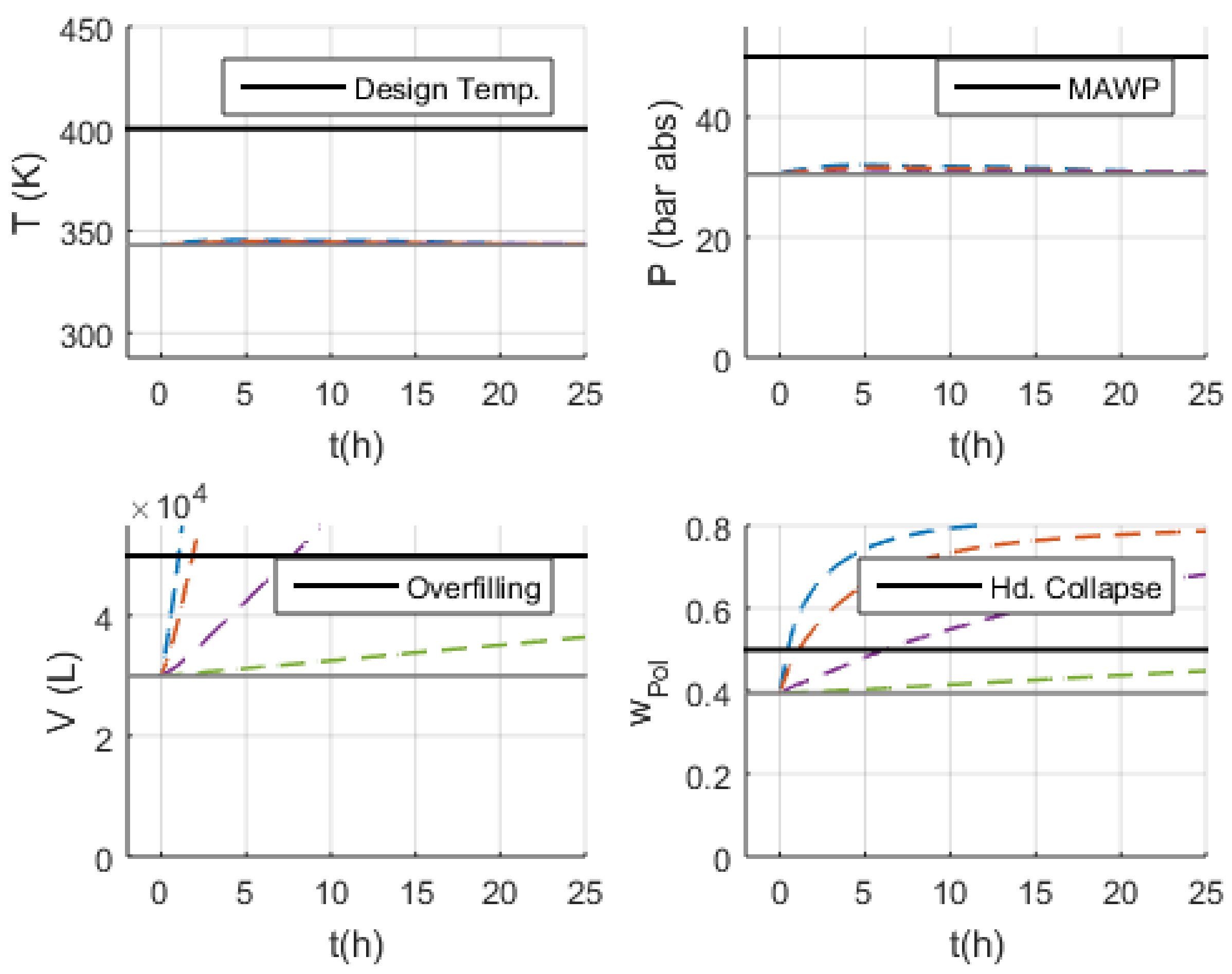
 ) no flow; (
  ) of normal flow; (
  ) of normal flow; (
  ) of normal flow; (
  ) normal.
) no flow; ( ) of normal flow; ( ) of normal flow; ( ) of normal flow; ( ) normal.
) normal.
) no flow; ( ) of normal flow; ( ) of normal flow; ( ) of normal flow; ( ) normal.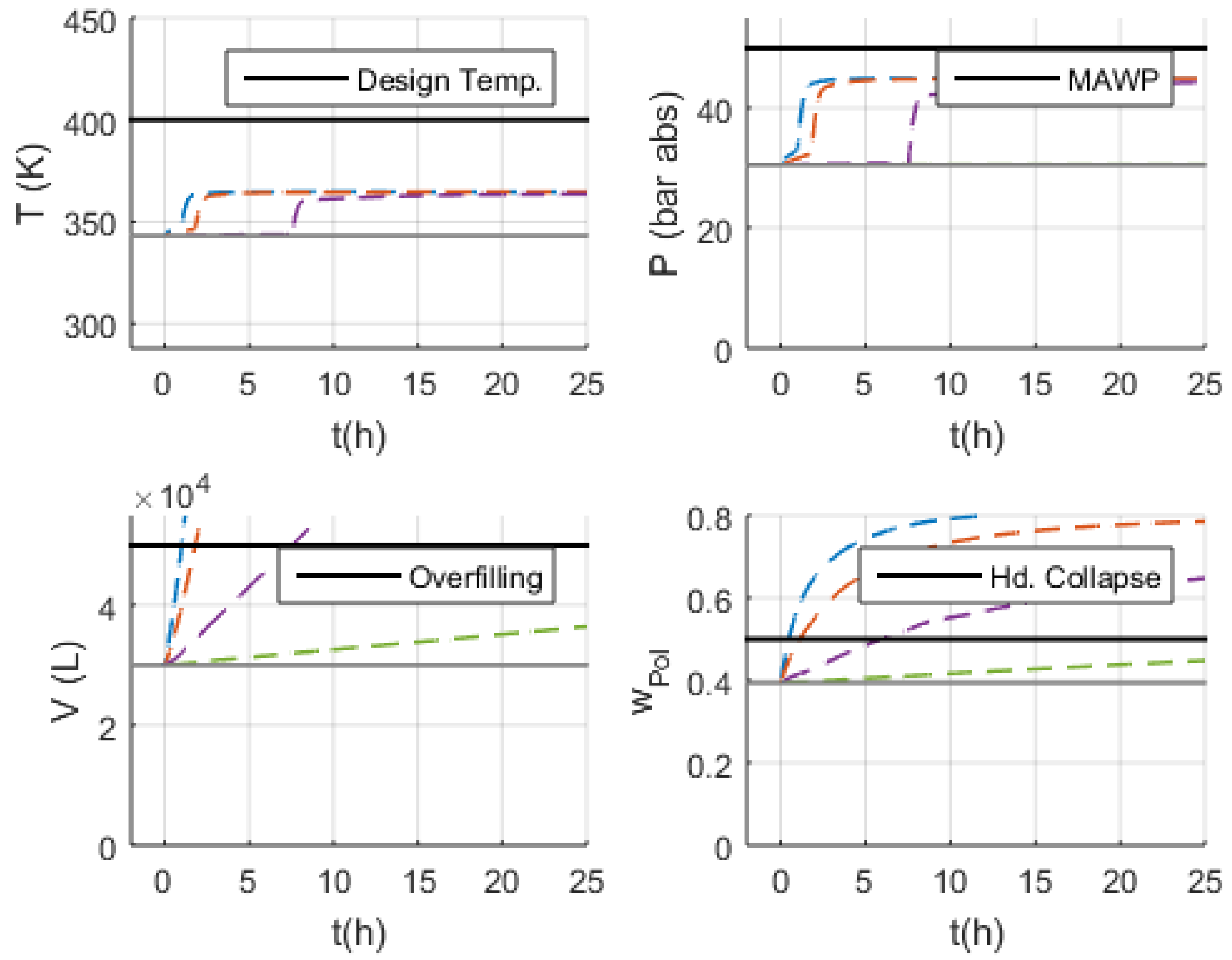
 ) no flow; (
  ) of normal flow; (
  ) of normal flow; (
  ) of normal flow; (
  ) normal.
) no flow; ( ) of normal flow; ( ) of normal flow; ( ) of normal flow; ( ) normal.
) normal.
) no flow; ( ) of normal flow; ( ) of normal flow; ( ) of normal flow; ( ) normal.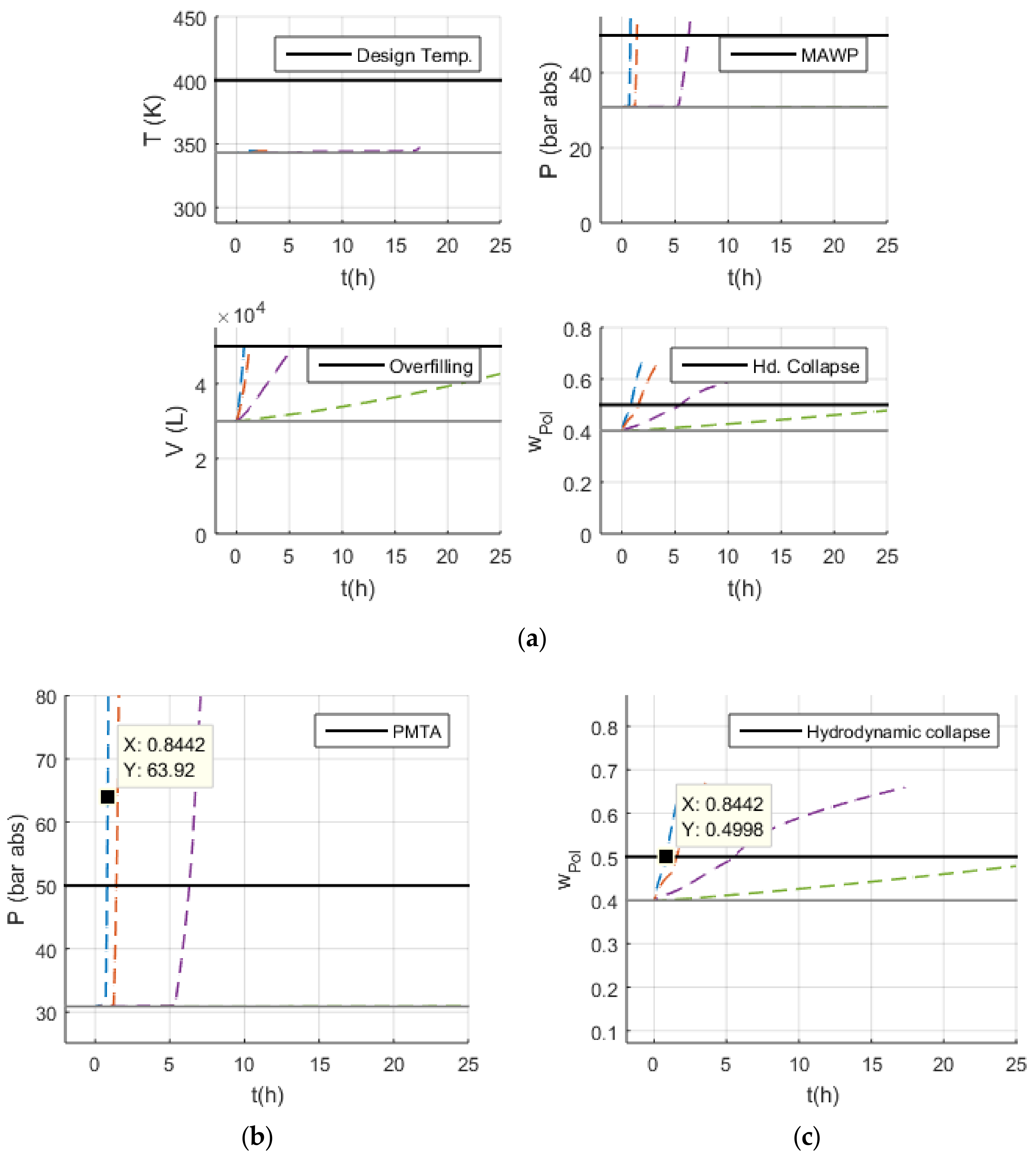
 ) maximum flow; (
  ) of normal flow; (
  ) of normal flow; (
  ) of normal flow; (
  ) normal.
) maximum flow; ( ) of normal flow; ( ) of normal flow; ( ) of normal flow; ( ) normal.
) normal.
) maximum flow; ( ) of normal flow; ( ) of normal flow; ( ) of normal flow; ( ) normal.
 ) maximum flow.
) maximum flow.
) maximum flow.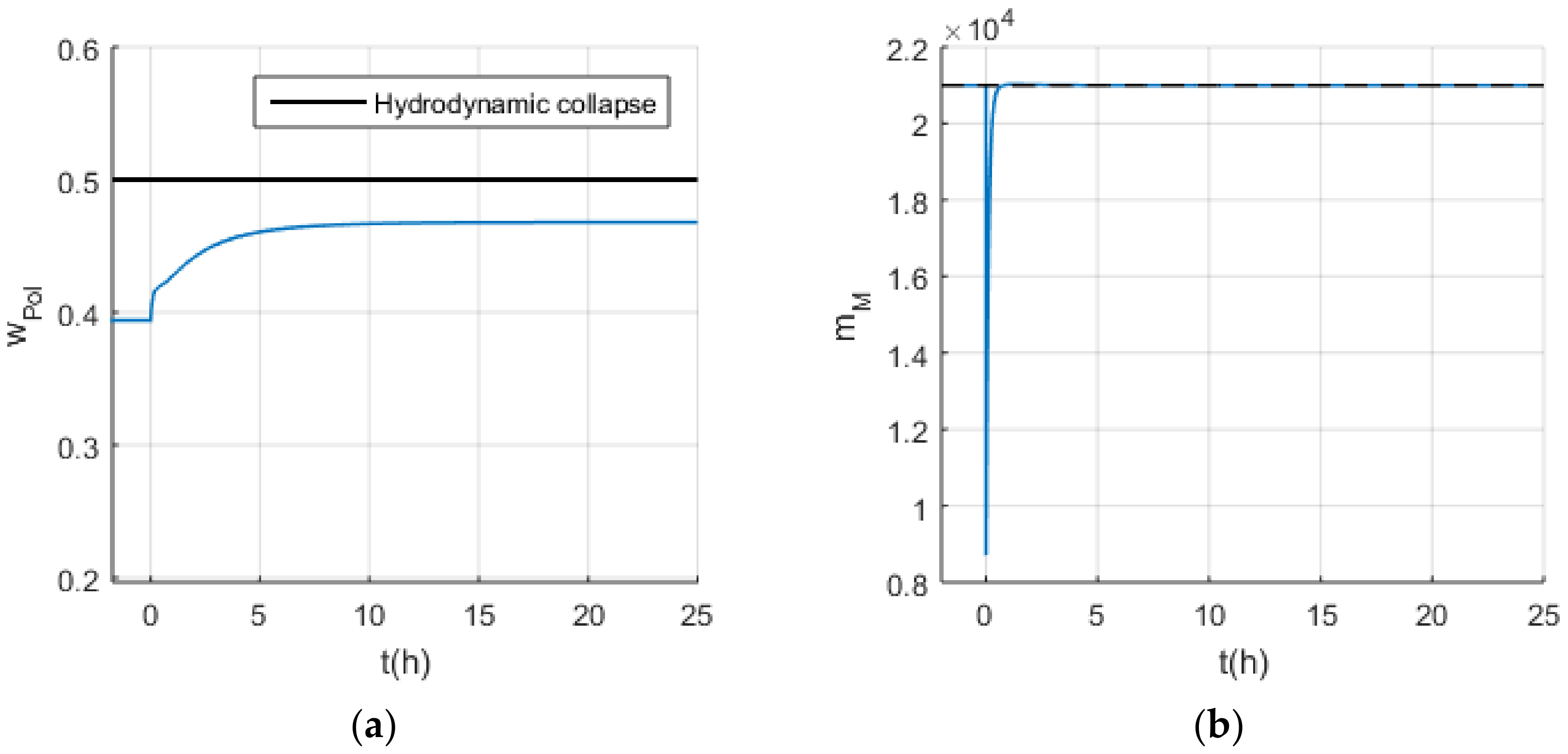


| Item | Function | Failure Mode |
|---|---|---|
| Input Streams | Add mass to the Process Node | No mass: pump failure, human error (valve inadvertently closed) |
| Less mass: control failure 1, plugging | ||
| More mass: control failure 1 | ||
| Other composition: Off-spec raw material | ||
| Add energy to the Process Node | Less energy: inlet temperature disturbance; failure of heat transfer control, control failure 1 | |
| More energy: inlet temperature disturbance, failure of heat transfer control, control failure 1 | ||
| Output Streams | Remove mass from the Process Node | No mass: pump failure, human error (valve inadvertently closed) |
| Less mass: control failure 1, plugging | ||
| More mass: control failure 1 | ||
| Remove energy from the Process Node | Coupled to mass balance 2, failure of heat transfer control |
| Item | Function | Failure Mode |
|---|---|---|
| Equipment External Walls | Contain mass | Corrosion. Design limits may depend on process parameters and devices. Occurrence of leaks. |
| Exchange a limited amount of energy | Fouling, scaling, and encrustation. | |
| Equipment Internal Walls | Contain mass | Corrosion. Design limits may depend on process parameters and devices. Occurrence of leaks. |
| Exchange a limited amount of energy | Fouling, scaling, and encrustation. |
| Nomenclature | |
|---|---|
| Cat | Catalyst stream |
| TEA | Triethyl aluminum stream |
| PEEB | Para-ethyl 4-ethoxybenzoate stream |
| H2 | Hydrogen stream |
| M | Monomer stream |
| M,Rec | Monomer recycle stream |
| M,Cond | Monomer stream to condenser |
| M,mkp | Monomer make-up stream |
| w | Water stream to condenser |
| s | Slurry stream from reactor |
| gas | Gas stream from separator |
| purge | Purge stream |
| Pol | Polymer stream |
| Item | Description | Function | Failure Mode | Simulation Reference |
|---|---|---|---|---|
| 1 | Monomer make-up stream | Add fresh monomer to the reactor | No mass: pump failure, valve inadvertently closed | S-1 |
| Less mass: control failure, plugging | S-2 | |||
| More mass: control failure | S-3 | |||
| Other composition: off-spec raw material (more propane) | Not discussed in the present paper | |||
| Add energy to the reactor | Less energy: lower inlet temperature | Not discussed in the present paper | ||
| More energy: higher inlet temperature | Not discussed in the present paper | |||
| 11 | Recycled monomer purge stream | Remove recycled monomer from the reactor | No mass: valve inadvertently closed | Not discussed in the present paper |
| Less mass: control failure | Not discussed in the present paper | |||
| More mass: control failure | S-35 |
Publisher’s Note: MDPI stays neutral with regard to jurisdictional claims in published maps and institutional affiliations. |
© 2022 by the authors. Licensee MDPI, Basel, Switzerland. This article is an open access article distributed under the terms and conditions of the Creative Commons Attribution (CC BY) license (https://creativecommons.org/licenses/by/4.0/).
Share and Cite
de Azevedo, J.P.A.; de Souza, M.B., Jr.; Pinto, J.C. Process Hazard Analysis Based on Modeling and Simulation Tools. Processes 2022, 10, 386. https://doi.org/10.3390/pr10020386
de Azevedo JPA, de Souza MB Jr., Pinto JC. Process Hazard Analysis Based on Modeling and Simulation Tools. Processes. 2022; 10(2):386. https://doi.org/10.3390/pr10020386
Chicago/Turabian Stylede Azevedo, Júlia Pinto Athanázio, Maurício Bezerra de Souza, Jr., and José Carlos Pinto. 2022. "Process Hazard Analysis Based on Modeling and Simulation Tools" Processes 10, no. 2: 386. https://doi.org/10.3390/pr10020386
APA Stylede Azevedo, J. P. A., de Souza, M. B., Jr., & Pinto, J. C. (2022). Process Hazard Analysis Based on Modeling and Simulation Tools. Processes, 10(2), 386. https://doi.org/10.3390/pr10020386