Article

An Extended Tissue-like P System Based on Membrane Systems and Quantum-Behaved Particle Swarm Optimization for Image Segmentation

1
School of Management Engineering, Shandong Jianzhu University, Jinan 250101, China
2
School of Business, Shandong Normal University, Jinan 250307, China
3
School of Management Science and Engineering, Shandong University of Finance and Economics, Jinan 250002, China
*
Author to whom correspondence should be addressed.
Processes 2022, 10(2), 287; https://doi.org/10.3390/pr10020287
Submission received: 8 November 2021 / Revised: 27 January 2022 / Accepted: 29 January 2022 / Published: 31 January 2022
(This article belongs to the Topic Bioreactors: Control, Optimization and Applications)

Abstract

:
An extended membrane system using a tissue-like P system with evolutional symport/antiport rules and a promoter/inhibitor, which is based on the evolutionary mechanism of quantum-behaved particle swarm optimization (QPSO) and improved QPSO, named CQPSO-ETP, is designed and developed in this paper. The purpose of CQPSO-ETP is to enhance the optimization performance of statistical network structure-based membrane-inspired evolutionary algorithms (SNS-based MIEAs) and the QPSO technique. In CQPSO-ETP, evolution rules with a promoter based on a standard QPSO mechanism are introduced to evolve objects, and evolution rules with an inhibitor based on an improved QPSO mechanism using self-adaptive selection, and cooperative evolutionary and logistic chaotic mapping methods, are adopted to avoid prematurity. The communication rules with a promoter/inhibitor for objects are introduced to achieve the exchange and sharing of information between different membranes. Under the control of the evolution and communication mechanism, the CQPSO-ETP can effectively improve the performance with the help of a distributed parallel computing model. The proposed CQPSO-ETP is compared with PSO, QPSO and two existing improved QPSO approaches which are conducted on eight classic numerical benchmark functions to verify the effectiveness. Furthermore, computational experiments which are made on eight tested images with three comparative clustering approaches are adopted, and the experimental results demonstrate the clustering validity of the proposed CQPSO-ETP.

1. Introduction

Membrane computing (MC) is an important branch of bio-inspired computing, which is initiated by Păun [1], and the computing models of membrane computing are also called membrane systems or P systems. P systems focus on abstracting some fundamental concept from the structure and functioning of the living cells, cell tissues or colonies of cells. Research shows that some P systems have the same computing power as Turing machines, or are more efficient, to some extent [2]. There are three classic computing models of P systems according to the structure of the membrane or cell arrangement in previous studies and researches, including cell-like P systems, tissue-like P systems and neural-like P systems [3]. Many variants of P systems based on biological facts, mathematical biological cells, theoretical computer science or application motivations have been presented for solving difficult optimization problems in real life [4,5].
In general, several variants of P systems on the theoretical development of MC that are mostly based on three classic P systems that recruit various ingredients, including energy, catalysts and mitosis, have been reported in previous studies and related works [6]. Many kinds of extended cell-like P systems have been reported in the literature, such as cell-like P systems with active membranes inspired in the mitosis process [7,8,9], cell-like P systems with evolutional symport/antiport rules inspired by the conservation law [10,11], and so on. Similarly, tissue-like P systems with evolutional symport/antiport rules are a class of computing modes based on cell inter-communication in tissues [6,12,13]. The interchange of objects between regions are determined by the existence of promoters or inhibitors, it is simply called tissue-like P systems with a promoter/inhibitor [14,15,16]. The multiset rewriting rules are introduced to tissue-like P systems based on the energy assumption, which names homeostasis tissue-like P systems [17,18]. Spiking neural-like P systems (SN P) are an important computing model of neural-like P systems [19]. Many variants of SN P systems have emerged, such as SN P systems with rules on synapses [20], SN P systems with multiple channels [21], SN P systems with anti-spikes [22], and other made changes on communication rules [23]. The analysis of computing power and computational efficiency for P systems and their variants is also an important part of studies and works [24].
Evolutionary computation (EC) based on the fundamental principles of biological evolution is an important branch of natural computing [25], which generally divided into two broad areas, evolutionary algorithms (EAs) and swarm intelligence (SI) [26]. Especially, EAs are inspired by natural selection and molecular genetics, consisting of classic EAs and recently developed EAs [27]. Classic EAs included genetic algorithms (GAs) [28], evolution strategies (ES) [29], evolutionary programming (EP) [30] and genetic programming (GP) [31]. Recently developed EAs contained a family of optimization algorithms, such as quantum-inspired evolutionary algorithms (QIEAS) [32], simulated annealing (SA) [33], differential evolution (DE) [34], and tabu search (TS) [35]. SI involved many kinds of meta-heuristic techniques, including particle swarm optimization (PSO) [36], ant colony optimization (ACO) [37], an artificial bee colony algorithm (ABC) [38], biogeography-based optimization (BBO) [39], and an artificial fish swarm algorithm [40]; these techniques have been widely used to solve many complicated problems [41].
The combination of MC and EC is an important application in studies of MC and EC [42], which is named evolutionary membrane computing (EMC) [43]. The parallel-distributed framework of MC and computing characteristics of EC, such as easy implementation, robust performance, are utilized to EMC in order to improve computation performance [44]. In this respect, two wide research areas of EMC have been studied, including membrane-inspired evolutionary algorithms (MIEAs), also called membrane algorithms (MAs), and the automated design of membrane computing models (ADMCM) [27]. Specially, MIEAs or MAs are outstanding instances in MC for approaching real-word applications [45], which can be classified into two categories according to different membrane structure: hierarchical membrane structure from cell-like P systems and network membrane structure from tissue-like P systems and neural-like P systems [46].
Furthermore, hierarchical structure based MIEAs, including a nested membrane structure (NMS) [47], one level membrane structure (OLMS) [48], hybrid membrane structure (HMS) [49] and dynamic membrane structure (DMS) [50], are the first kind of EMC. NMS-based MIEAs are designed to integrate cell-like P systems with different meta-heuristic techniques, such as GA [51], DE [52,53], ACO [54], and so on [55,56]. OLMS-based MIEAs are proposed to combine cell-like P systems and different algorithms in a membrane (AIM), such as GA [57], DE [58], PSO [59,60], ACO [61], and QIEAS [62]. Due to combination possibilities of a hybrid membrane structure, HMS-based MIEAs based on the membrane structure of NMS and OLMS are presented. However, the complexity and difficulty of a hybrid structure are limited to the development of HMS-based MIEAs [63,64]. The dynamic membrane structure of DMS-based MIEAs is different from the static membrane structure of NMS-based MIEAs, OLMS-based MIEAs and HMS-based MIEAs. Moreover, the hierarchical membrane structure of DMS-based MIEAs can be changed with active membranes during the evolution process [65,66].
The network structure based MIEAs, including the statistical network structure (SNS) and dynamical network structure (DNS), are the second kind of EMC [67]. SNS-based MIEAs are presented by using tissue-like P systems or neural-like P systems with various network topologies [68]. Various meta-heuristic algorithms, such as GA [69], DE [70] and its variants [71,72], PSO [73,74], ABC [75], and BBO [76], are usually introduced to SNS-based MIEAs as the basic evolutionary operation in the cell or neural [77,78,79,80,81]. The membrane structure in DNS-based MIEAs can be dynamically changed according to communication channel rules, and this class of MIEAs, with an extended membrane structure, has great potential for solving complex problems [82,83]. For another kind of EMC, ADMCMs are designed to overcome the complex programmability of membrane-based modes, and the automated synthesis of computing models by applying various meta-heuristic methods can be obtained through this class of EMC [84,85,86]. Three important research topics of ADMCM have been investigated, including abstract rewriting systems on multisets (ARSM) [87], parameter optimization of P system models (POPSM) [88] and automatic design of P systems (ADPS) [89,90,91].
Quantum-behaved particle swarm optimization (QPSO) is a variant of PSO which was initiated by Sun in 2004 [92], and the sampling space of QPSO covers the whole search space due to the probabilities of potential well models [93]. It has been proved that the global search ability of QPSO has been improved more than classic PSO [94]. Although QPSO has been shown a greater potential than traditional EC [95], it still has some limitations in the sample test set, such as being easily trapped into local optima and exhibited prematurity [96]. Tissue-like P systems are a kind of classic computing model in MC, and the underlying membrane structure of tissue-like P systems can be abstracted to an arbitrary graph in mathematics compared with cell-like P systems [97]. The parallel-distributed framework, particularly the membrane structure, and evolution–communication mechanism of tissue-like P systems can be used to improve the performance of EC. Therefore, the tissue-like P system with evolutional symport/antiport rules and a promoter/inhibitor is introduced to enhance the optimization performance of QPSO and to overcome the limitation as we mentioned above.
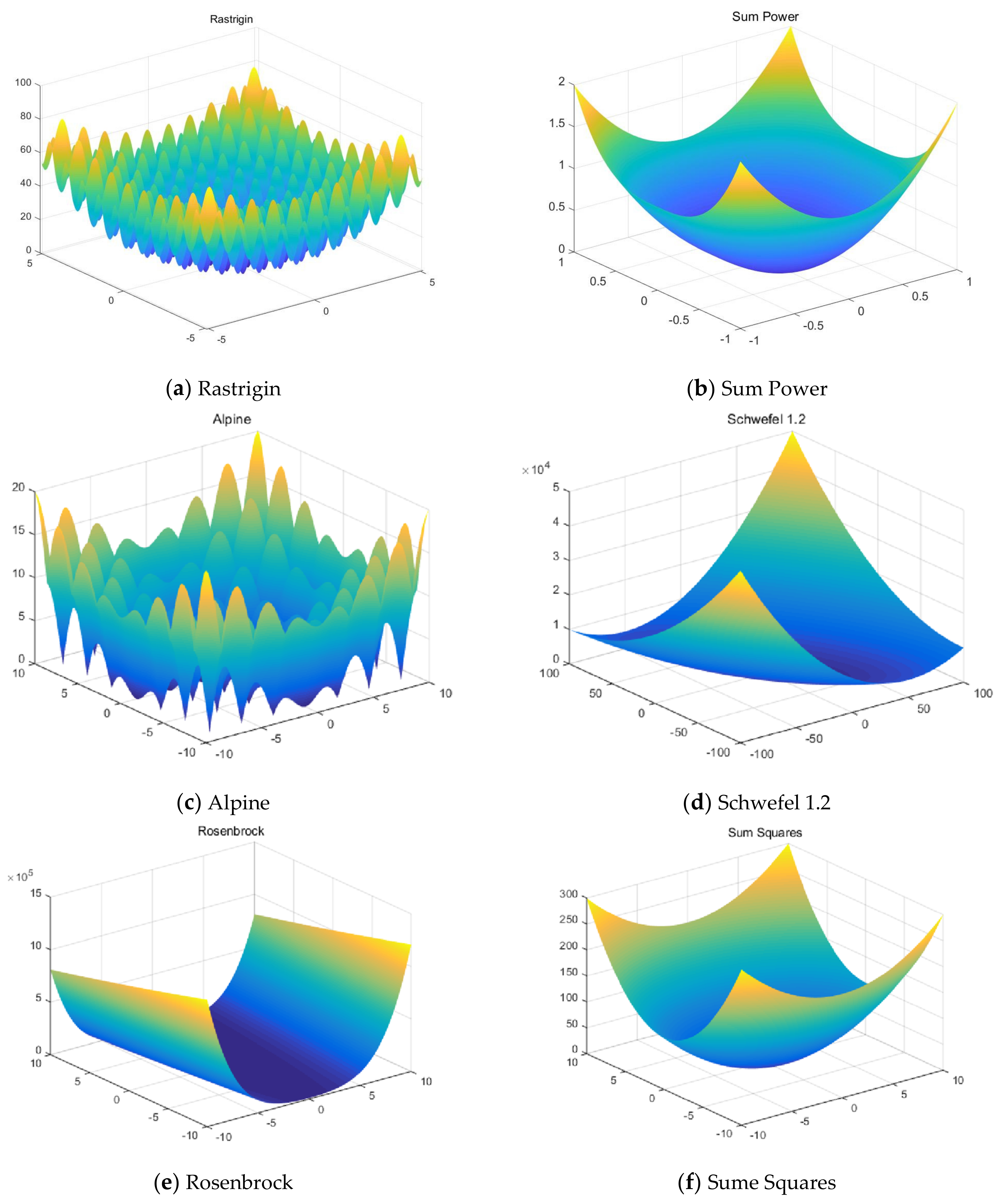
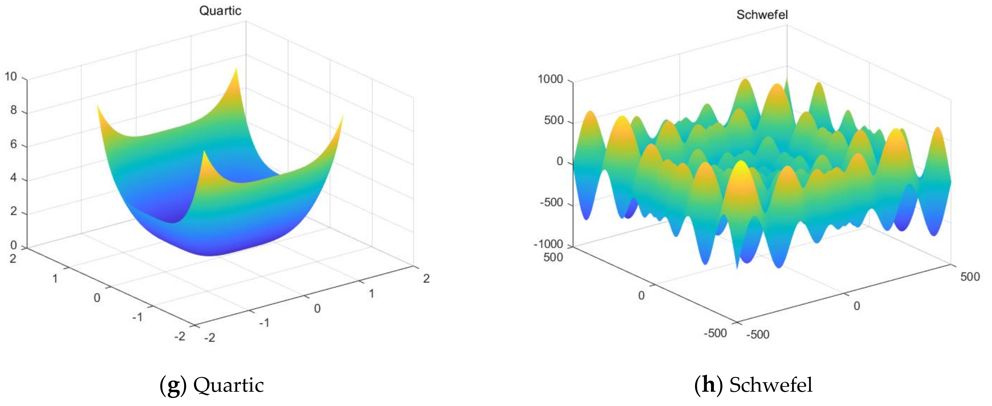
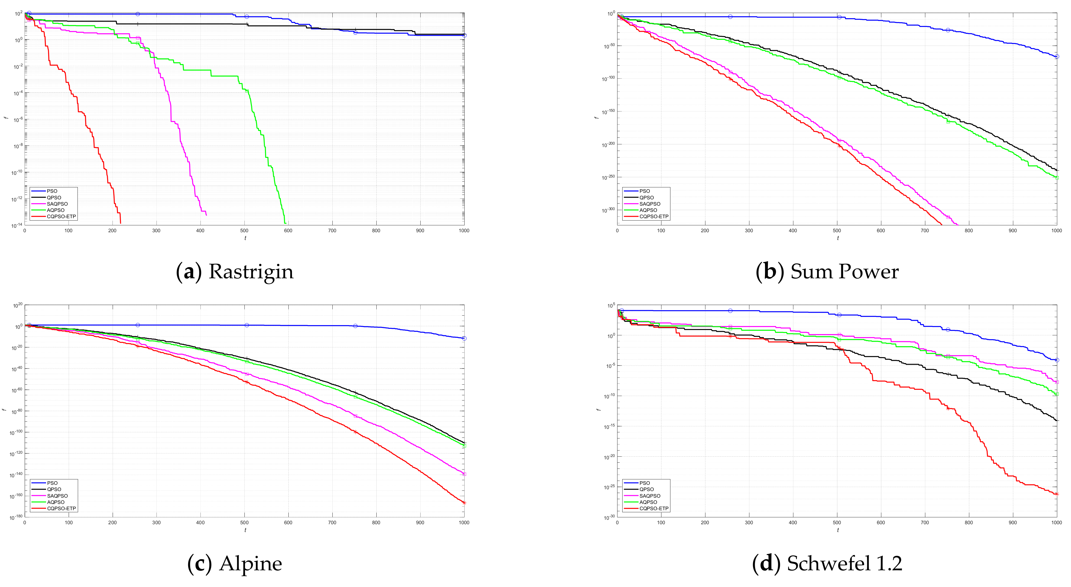
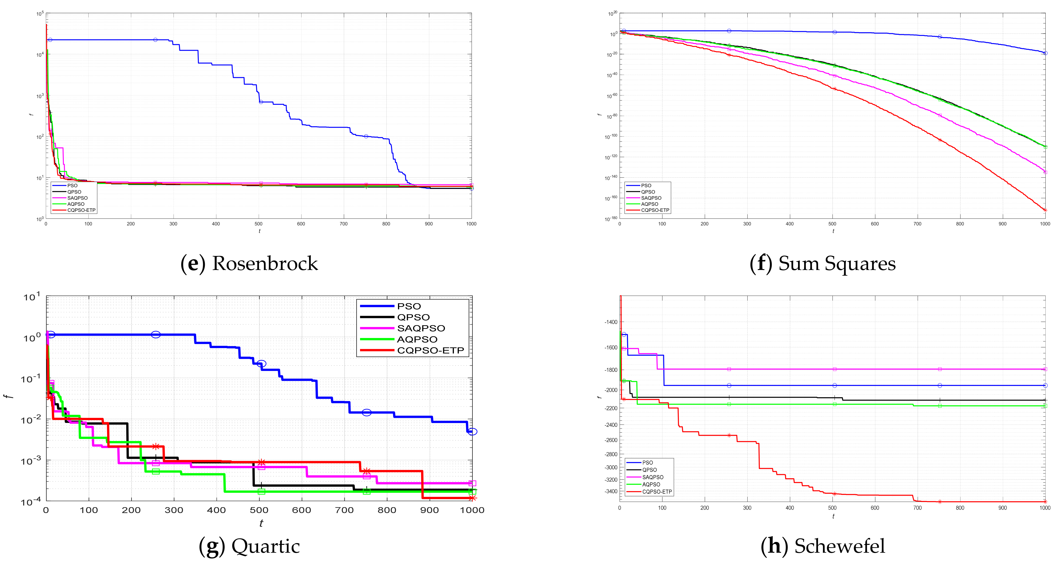
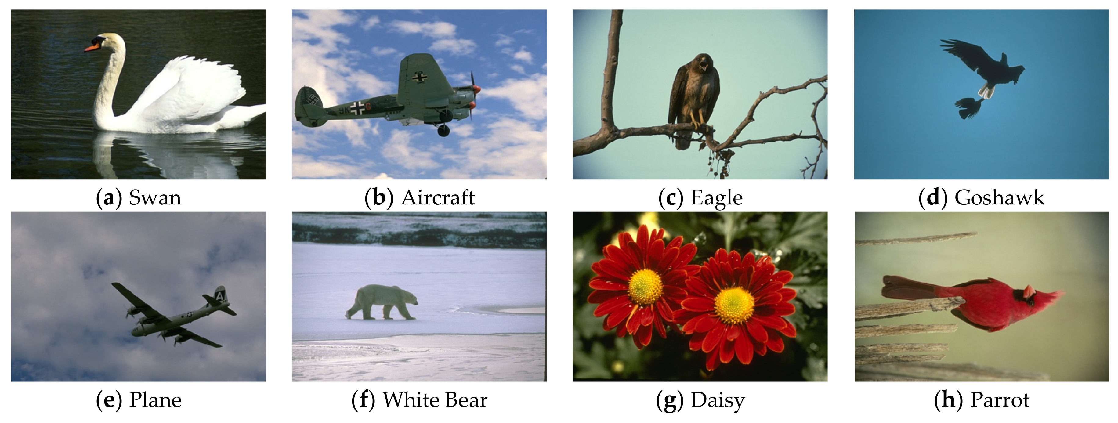
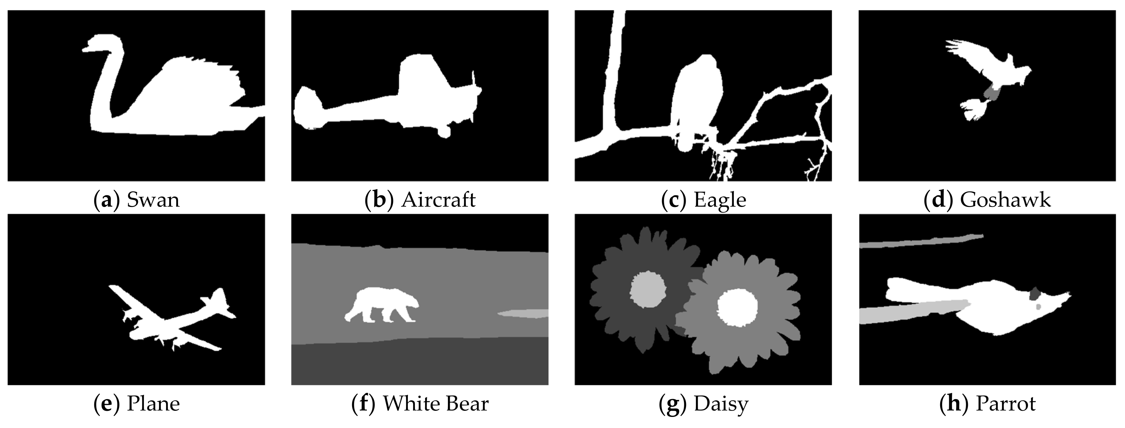
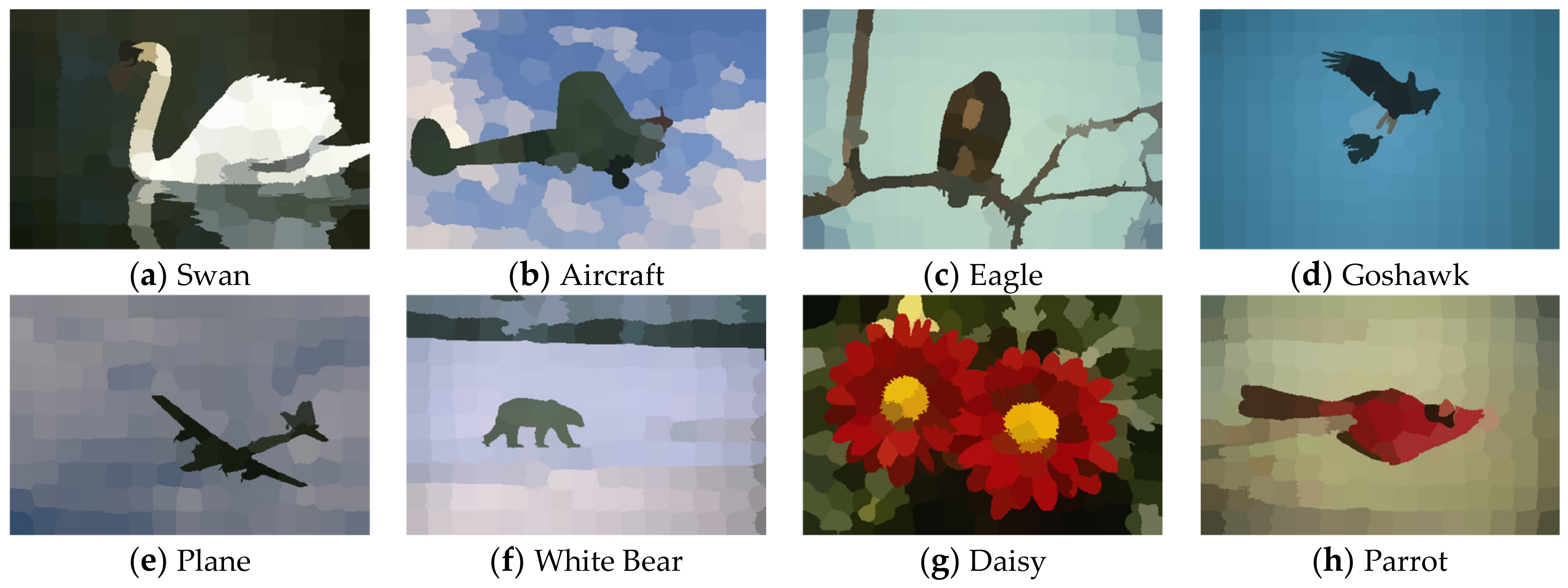
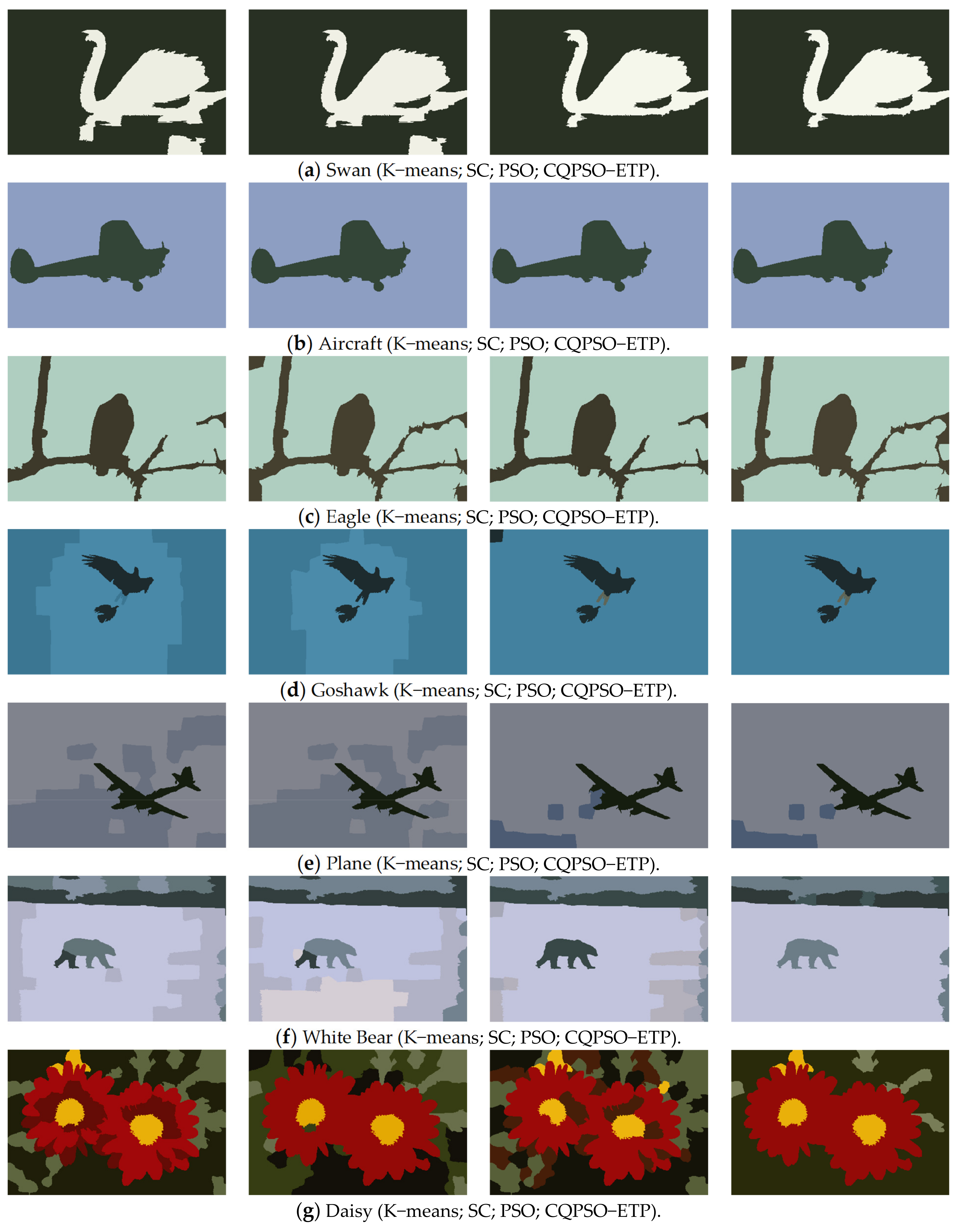
This work focuses on the development of a membrane computing model in SNS-based MIEAs to solve some optimization problems and image segmentation problems, which is based on the evolution mechanism of QPSO and improved QPSO, and the evolution–communication mechanism of the tissue-like P system. An extended tissue-like P system based on the evolution–communication mechanism of the tissue-like P system, with evolutional symport/antiport rules and a promoter/inhibitor, and an evolutionary mechanism of QPSO and improved QPSO is proposed. It is one kind of SNS-based MIEA, and simply named CQPSO-ETP. Evolutional symport/antiport rules and a promoter/inhibitor are introduced to this extended P system in order to adjust the executing sequence of evolution–communication rules. In CQPSO-ETP, two kinds of evolution rules with a promoter and inhibitor for objects based on different generating strategies for local attractor are described, one of the evolution rules with a promoter is based on the evolutionary mechanism of the standard QPSO technique. Another evolution rule with an inhibitor is based on the evolutionary mechanism of an improved QPSO technique using self-adaptive selection, cooperative evolution and a logistic chaotic mapping method. The communication for objects in different membranes or regions is achieved by the execution of communication rules with a promoter and inhibitor for objects. At last, the proposed CQPSO-ETP is evaluated on eight classic numerical benchmark functions and compared with PSO, QPSO, and two existing improved QPSO optimization approaches to verify the validity and performance. Furthermore, this extended P system is compared with three classic existing clustering techniques, and comparison experiments on eight tested images from image segmentation problems are performed to validate the clustering efficiency of this proposed CQPSO-ETP.
The rest of this paper is organized as follows: the basic framework of the tissue-like P system with evolutional symport/antiport rules and a promoter/inhibitor are described in Section 2. More details about the evolutionary mechanism of QPSO and improved QPSO are given in Section 3. The extended tissue-like P system based on the tissue-like P system with evolutional symport/antiport rules and a promoter/inhibitor, and QPSO and improved QPSO are proposed in Section 4, and evolution and communication rules with a promoter/inhibitor for objects are described in more details in this section. Experimental results and analysis on eight classic numerical benchmark functions with four comparative approaches are reported in Section 5. Section 6 gives the experimental results and discussion which are made on eight tested images with three classic existing clustering approaches to evaluate the clustering efficiency of this proposed extended tissue-like P system. Section 7 provides some conclusions and outlines future research directions.

2. The Tissue-like P System

2.1. The Tissue-like P System with Evolutioanl Symport/Antiport Rules

In the computing model of a basic tissue-like P system with symport/antiport rules and its variants, different membranes or regions exchange and share information or objects according to the standard symport/antiport rules, but the objects are not modified during this communication process. In fact, this communication method only changed the place of the objects in the system, but did not change the chemical properties of the objects. Chemical substances are modified in the cell biology when the substances enter or exit in different membranes, and this biological phenomenon is called the evolution of substances. Therefore, the evolution idea for objects during the communication process is inspired from the evolution of substances which can be considered in the tissue-like P system, then the objects can be modified through some evolution rules. A tissue-like P system with an evolutional symport/antiport is described as a tuple in the following [24]:
Π = Γ , ε , μ , ω 1 , , ω m , R , σ o u t ,
where
(1)
Γ is a non-empty finite alphabet of objects, each alphabet represents an object;
(2)
ε is a set of initial objects located in the environment;
(3)
μ is the membrane structure of the system that consisting m membranes;
(4)
ω 1 , , ω m are finite multisets of the initial objects over Γ ;
(5)
R is a finite set of evolution rules of the following forms:
<1>
 Evolutional symport rules: u i j i u j , where 1 < i m , 0 < j m , i j , u Γ + , u Γ * or i = 0 , 1 < j m , u Γ + , u Γ * ;
<2>
 Evolutional antiport rules: u i v j v i u j where 0 i j m , u , v Γ + , u , v Γ * ;
(6)
σ o u t is the output region or membrane in the tissue-like P system with the evolutional symport/antiport rules, σ o u t { σ 0 , σ 1 , , σ m } , where the membrane i ( 1 i m ) is simply denoted by σ i , and environment is usually denoted by σ 0 .
An evolutional symport rule, u i j i u j , provides a new kind of communication way from membrane i to membrane j . It only can be executed on a moment if there is a membrane in a configuration which contains a multiset of objects that are denoted by u ( u Γ ). When the evolutional symport rule associated with membrane i ( 1 i m ) and membrane j ( 1 j m ) is applied, the objects u in membrane i are evolved to the new objects which are denoted by u ( u Γ ), and are sent to membrane j at the same time. Note that objects u in membrane i are consumed during this evolutional communication process. An evolutional antiport rule, u i v j v i u j , provides a new kind of communication way from membrane i to membrane j . It only can be executed on a moment if there is a membrane in a configuration which contains a multiset of objects u , and another membrane which contains a multiset of objects that are denoted by v ( v Γ ). When the evolutional antiport rule associated with membrane i and membrane j is applied, the objects u in membrane i are evolved to the new objects u and are sent to membrane j . At the same time, the objects v in membrane j are evolved to the new objects that are denoted by v ( v Γ ) and are sent to membrane i . Note that objects u in membrane i and object v in membrane j are consumed during this evolutional communication process. Especially, if the objects are not modified but have just changed their place during the communication process in the tissue-like P system, then it is a particular case of the tissue-like P system with evolutional symport/antiport rules, and simply called the tissue-like P system with symport/antiport rules.

2.2. The Tissue-like P System with Evolutional Symport/Antiport Rules and Promoter/Inhibitor

In general, the evolutional rules in the traditional tissue-like P system with evolutional symport/antiport rules are adopted in this work, which are applied in a maximal and spontaneous parallel manner. The evolutional symport/antiport rules for objects are only executed on this moment when the objects exist in the membranes or environment. Therefore, the promoter and inhibitor are introduced to dynamically change the evolution–communication process of this system in order to adjust the execution sequence rather than the uncertain working manner of the traditional P system. Therefore, a recognizer tissue-like P system with evolutional symport/antiport rules and a promoter/inhibitor is defined, and simply called an ETP system. An ETP system is a tuple which can be described in the following [15]:
Π = Γ , ε , μ , ω 1 , , ω m , R , σ o u t ,
where
(1)
Γ is a finite non-empty alphabet of objects;
(2)
ε is a set of initial objects located in the environment;
(3)
μ is the membrane structure consisting of m membranes;
(4)
ω 1 , , ω m are finite multisets of initial objects over Γ ;
(5)
R is a finite set of rules that contained two kinds of evolution rules, i.e., evolutional symport rules with a promoter/inhibitor and evolutional antiport rules with a promoter/inhibitor, which are described in following forms:
<1>
 Evolutional symport rules: u p i j i u j , where 0 i j m , u Γ + , u Γ * , p Γ ;
<2>
 Evolutional antiport rules: u p i v j v i u j , where 0 i j m , u , v Γ + , u , v Γ * , p Γ ;
(6)
σ o u t is the output region or membrane in the ETP system, where σ o u t { σ 0 , σ 1 , , σ m } .
In ETP system, an evolutional symport rule with a promoter/inhibitor, u p i j i u j provides a new kind of communication pathway between membrane i and membrane j . It can be executed on a moment if there is a membrane in a configuration which not only contains a multiset of objects, u ( u Γ ), but also contains the promoter/inhibitor objects that are denoted by p . Specially, promoter/inhibitor objects p in the subscript are the promoter or inhibitor of the form p = p * and p = ¬ p * , where p * represents the promoter and ¬ p * represents the inhibitor. When the evolutional antiport rule with the promoter/inhibitor associated with membrane i and membrane j is applied, the objects u with the promoter/inhibitor objects p in membrane i are evolved to the new objects u and are sent to membrane j . Note that the objects u and promoter/inhibitor objects p in membrane i are consumed during this evolutional communication process. An evolutional antiport rule with a promoter/inhibitor, u p i v j v i u j provides a new kind of communication way between membrane i to membrane j . It can be executed on a moment if there is a membrane in a configuration which contains a multiset of objects u and promoter/inhibitor objects p , and another membrane in the same configuration which contains a multiset of objects v ( v Γ ). When the evolutional antiport rule with the promoter/inhibitor associated with membrane i and membrane j is applied, the objects u with the promoter/inhibitor objects p in membrane i are evolved to the new objects u and are sent to membrane j . And the objects v in membrane j are evolved to the new objects v and are sent to membrane i at the same time. Note that the objects u and the promoter/inhibitor objects p in membrane i , and the objects v in membrane j are consumed during this evolutional communication process.
An ETP system with the degree m ( m 1 ) can be regarded as a set of m cells or membranes which are labeled from 1 to m , and the environment is usually labeled by 0 . Traditionally, the mathematics structure of the ETP system can be viewed as a graph in topology. A configuration of the ETP system at any time can be described by all multisets of objects over Γ with corresponding cells or membranes in the system, and the multisets of objects over Γ / ε with the environment at the same time. All objects can be evolved through a maximally parallel manner at each step. The ETP system started from the initial configuration and evolved to the execution of the evolutional symport/antiport rules with a promoter/inhibitor, as described above, then a sequence of consecutive configurations will be generated and changed during this evolution process. If no rules can be executed in the system, the computation of the ETP system will be stopped. The end of the configuration is called the halting configuration. Note that only the halting configuration will gives the final computational results obtained from the system, which are usually encoded to the number of the objects placed in the output region or membrane σ o u t .

3. The Improved Quantum-Behaved Particle Swarm Optimization

3.1. The Standard Quantum-Behaved Particle Swarm Optimization

The Quantum-behaved particle swarm optimization (QPSO) is inspired by the concepts of quantum physics and PSO techniques. As a probabilistic global optimization technique, the basic principle of QPSO is different from the basic principle of the PSO technique. Each particle only depends on the information of the local attractor and local best to adjust the flight trajectory. Compared with traditional PSO, the velocity of a particle is replaced by the local attractor, and the local attractor contains two parts, including self-cognition and social-cognition. Therefore, each particle moves according to the local attractor and the mean position of the local best in the whole population, and will attract to the local attractor based on the position of the local best and global best in the search space. The local attractor is denoted by z i t of i -th particle at iteration t , which is determined by (1) in the following [98]:
z i j t = φ p i j t + 1 φ p g j t ,   for j = 1 , 2 , , D ,
where φ is a uniform random number which is distributed on the interval from 0 to 1, φ U 0 , 1 . D is the dimension of the search space. p i t is the position of the local best for particle i at iteration t , and p g t is the position of the global best in the whole population of the particle at iteration t . The z i j t is a stochastic point on the j -th ( 1 j D ) dimension which was generated from the point p i j t of the local best position, p i t on the j -th dimension, and the point p g j t of the global best position p g t on the j -th dimension. The new point x i j of position x i of the i -th particle at iteration t + 1 is defined by (2) in the following [98]
x i j t + 1 = z i j t ± γ p m j t x i j t ln 1 / η , j = 1 , 2 , , D ,
where η is a uniform random number which is distributed on the interval from 0 to 1, η U 0 , 1 . γ is the adjustment parameter to adjust the search speed of the i -th particle, and the named contraction–expansion coefficient. p m t is the position of the mean best based on the average of the local best for all particles in the whole population at iteration t , and it is also used to enhance the collaborative ability and global search ability for particles. The position p m t of the mean best at iteration t is given by (3) in the following [92],
p m t = 1 N i = 1 N p i t = 1 N i = 1 N p i 1 t , 1 N i = 1 N p i 2 t , , 1 N i = 1 N p i D t ,
The Equation (3) can be simplified as shown in (4) in the following [92],
p m j t = 1 N i = 1 N p i j t , j = 1 , 2 , , D ,
where N is the total number of particles in the population.
The computing procedure of the QPSO technique can be described as follows:
(1)
Initialization. Initialize the position of all particles with random numbers in the search space;
(2)
Update. Update the position of the local best and the global best for each particle, and compute the position of the mean best based on the position of the local best for all particles in the population according to Equation (3) or (4);
(3)
Evaluation. Update the local attractor and position for each particle according to Equations (1) and (2), and evaluate the fitness function which is used to select the local best and global best in the population;
(4)
Termination. The steps (2)–(3) will be implemented repeatedly with an iterative form until the termination criterion is satisfied, and the termination criterion of the QPSO technique is to evaluate whether the maximum number of iterations is reached.

3.2. The Cooperative Evolutionary Self-Adaptive Quantum-Behaved Particle Swarm Optimization

In this section, an improved QPSO is presented to enhance the global search ability and to avoid prematurity, which is simply named CQPSO. The self-adaptive selection method is introduced to dynamically adjust the values of acceleration factors in the updating of the local attractor, and the diversity function is adopted to help particles escape to the local optimum. Then the cooperative evolutionary strategy is used for the updating of the local attractor in the QPSO technique, and to increase the probability of discovering the global optimum in the search space. At last, a logistic chaotic mapping method is introduced to generate the chaotic sequence of random parameters in the position updating of particles. More details about the CQPSO technique are discussed in the following.

3.2.1. Self-Adaptive Selection

In the classic QPSO technique as we mentioned above, the local attractor z i of the i -th particle is determined by the position of the local best and global best, according to the Equation (1). Based on this, the regulation parameter φ i of the i -th particle is the key factor to balance the influence of the local best and global best. Therefore, the acceleration factors are introduced to generate the regulation parameter in the updating of the local attractor, which are given by (5) in the following [93],
φ i = c 1 r 1 c 1 r 1 + c 2 r 2 ,  
where r 1 and r 2 are uniform random numbers which are distributed on the interval from 0 to 1, r 1 U 0 , 1 , and r 2 U 0 , 1 . c 1 and c 2 are two acceleration factors in the updating of the regulation parameter. The acceleration factors have a considerable impact both on the convergence speed and accuracy of the QPSO technique. Therefore, the diversity function, which is denoted by D , is introduced to dynamically adjust the acceleration factors in order to avoid prematurity and to enhance the global search ability. The diversity function is shown in (6) in the following [93],
D = min f g , f a v g max f g , f a v g ,
where f g is the fitness values of the current global best in the population. f a v g is the average of fitness values for all the current position of the particles. Thus the maximum and minimum of diversity function D is 0 and 1 through Equation (6), especially if D = 1 , which means the population diversity of the particles is poor, and if D 1 , which means the population diversity of particles is good [93].
The position of the particle is far away from the position of the global best in the search space at the early stage. Then the particle adjusts the direction of the flight trajectory though the influence of the local attractor and mean best. Therefore, the position of the particle is gradually close to the position of the global best in the search space. The diversity function D , as we mentioned above, is introduced to dynamically adjust the values of the corresponding acceleration factor c 1 and c 2 , which is based on the proximity of the current position and global best in the population. The corresponding acceleration factors c 1 and c 2 are given by (7) in the following [93],
c i = c max c min tan 0.875 t max t t max 0.6 + c min , D > ζ c max c min t max t t max + c min , D ζ , i = 1 , 2 ,
where c min and c max are the minimum and maximum of the acceleration factor. t max is the maximum number of iterations. ζ is a predefined threshold of acceleration factors.

3.2.2. Cooperative Evolutionary

In the traditional QPSO technique, the local attractor of each particle is determined by the position of the local best and global best in the population. Furthermore, the population diversity of particles decreases under the guidance of the local attractor during the optimization process [99]. The position of the particles will be limited in a rectangle, the vertices of which are the position of the global best and local best, with the decreasing of the local attractor in the possible distribution space. Then particles will be easily trapped into the local optimum and appear prematurely. Therefore, the modification of Equation (1) is given in (8) in the following [99],
z i j t = φ i t p i j t + 1 φ i t p r 1 j t + Δ i j t , j = 1 , 2 , , D
where φ i t is a sequence number that is generated by Equation (5) at iteration t . p r 1 t is the position of the local best for particle r 1 , it can be randomly selected from the population of particles at iteration t . Δ i t = Δ i 1 t , Δ i 2 t , , Δ i D t is a perturbation vector at iteration t , which is given by (9) in the following [99],
Δ i t = ψ i t p r 2 t p g t ,
where ψ i t = ξ i t t / t max 0.5 , ξ is a uniform random number which is distributed on the interval from 0 to 1. t max is the maximum number of iterations. p r 2 t is the position of the local best for particle r 2 , which is randomly selected from the population of particles at iteration t ; note that i r 1 r 2 .

3.2.3. Logistic Chaotic Mapping

A logistic map, which was developed by May [100], is a classic kind of chaotic mapping method. And the chaotic variant c h t + 1 at iteration t + 1 , based on the logistic mapping method, is given by (10) in the following [101]
c h t + 1 = ς c h t 1 c h t , c h t 0 , 1   ,
where c h t is the chaotic number at iteration t , for c h 0 0 , 0.25 , 0.5 , 0.75 , 1.0 . ς is the control parameter, also called the chaotic coefficient, which is used to adjust the chaotic behavior of the chaotic variant c h t at iteration t , for ς 0 , + . If 3.5699 ς 4 , and the Lyapunov exponent of logistic map is greater than 0 , it means that the chaotic system is in a stable state at iteration t . The values of the chaotic variant based on varying values of the chaotic coefficient are shown in Figure 1a. Thus, a random sequence of the chaotic variant, which is generated by Equation (10), is distributed on the interval from 0 and 1 with some features, such as ergodicity, nonlinear, random similarity. A logistic chaotic map sequence of a chaotic variant after 100 iterations is given in Figure 1b.
In the position updating of particles in the QPSO technique, η is a uniform random number which is distributed on the interval from 0 to 1 through Equation (2), η U 0 , 1 . Therefore, the logistic mapping method, as we mentioned above, is adopted to generate the random parameter in Equation (2), it can help particles to explore the vicinity region of a potential solution by oscillating in the search space compared with the random generation method. The modification of the random parameter η at iteration t + 1 is given in (11) in the following
η i t + 1 = ς η i t 1 η i t ,   η i t 0 , 1 ,
where η i t is the values of parameter η for the i -th particle at iteration t through Equation (2), for η i 0 0 , 0.25 , 0.5 , 0.75 , 1.0 . Usually, in order to ensure the stability of the chaotic system, the value of the chaotic coefficient ς is set to 4.

4. The Proposed CQPSO-ETP

In this section, an extended tissue-like P system based on the evolution–communication mechanism of ETP and the evolution mechanism of QPSO and improved QPSO is proposed, and simply named CQPSO-ETP. The evolutionary mechanism for objects and communication mechanism for global objects are introduced in this extended P system. The rest of this section is organized in the following. Firstly, the general framework of this extended tissue-like P system is described, and the basic membrane structure is given in more details. Secondly, the evolution mechanism of QPSO and CQPSO and the evolution-communication mechanism of a tissue-like P system with evolutional symport/antiport rules and a promoter/inhibitor are introduced in the CQPSO-ETP to improve the performance of the extended P system. The computation of the proposed CQPSO-ETP is given in the following content. The complexity analysis of the CQPSO-ETP is described in the last parts.

4.1. The General Framework of CQPSO-ETP

The general framework of CQPSO-ETP is similar to the tissue-like P system with evolutional symport/antiport rules and a promoter/inhibitor. However, the rules for objects in the CQPSO-ETP are divided into two kinds of rules for objects, including the evolution rules for objects and communication rules for global objects. The membranes in the CQPSO-ETP system, are labeled from 1 to m , and simply denoted by σ 1 , σ 2 , , σ m . Respectively, CQPSO-ETP is a tuple which can be formally described in the following,
Π = Γ , μ , ω 1 , , ω m , R , R , σ o u t ,
where
(1)
Γ is a finite non-empty alphabet of objects;
(2)
μ is the membrane structure of CQPSO-ETP consisting of m membranes;
(3)
ω 1 , , ω m are finite multisets of initial objects in the membranes, with ω i Γ , for 1 i m ;
(4)
R represents finite sets of evolution rules in the CQPSO-ETP, R = R 1 , R 2 , , R m . Where R i ( 1 i m ) represents a finite set of evolution rules for objects associated with membrane i . Furthermore, the evolution rules R i of membrane i are of the form: R i = u p v , for u , v , p Γ . When the evolution rule is applied, object u is evolved to object v with the promoter/inhibitor p in the same membrane. In particular, p is the promoter or inhibitor of the form p = p * and p = ¬ p * , where p * represents the promoter and ¬ p * represents the inhibitor.
(5)
R represents finite sets of communication rules in the CQPSO-ETP, R = R 1 , R 2 , , R m . R i j ( 1 i j m ) represents a finite set of commutation rules for global objects associated with membrane i to membrane j . The form of the communication rules is also the same as the form of the evolutional symport/antiport rules, which can be described in the form: R i j = u q i j i u j or R i j = u q i v j v i u j , for u , v , u , v , q Γ , q p , where q is the promoter or inhibitor of the form q = q * and q = ¬ q * , q * represents the promoter, and ¬ q * represents the inhibitor; note that p q .
(6)
σ o u t is the output membrane in the CQPSO-ETP, where σ o u t { σ 1 , , σ m } or σ o u t = σ 0 
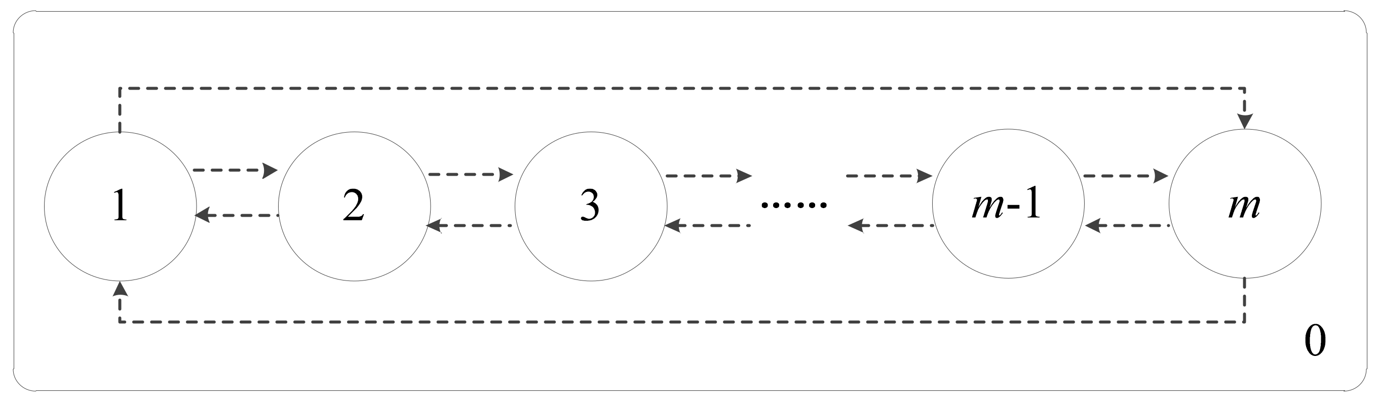
. Once the computation is completed, the computational results or objects in the output membrane will be transported to the environment. The membrane structure of CQPSO-ETP is especially graphically depicted in Figure 2.
In Figure 2, the CQPSO-ETP contains m membranes, which are simply denoted by σ 1 , σ 2 , , σ m . σ i ( 1 i m ) is called the elementary membrane and does not contain any other membrane, and σ 0 represents the environment that is around the elementary membrane. All membranes work in a parallel way, and each membrane can be viewed as a parallel computing unit. The elementary membrane only communicated with its neighboring membranes, which are the adjacent membranes of the current membrane in the graphical structure of Figure 2. This communication relationship is defined by the dotted lines, the exchange and sharing of information in different membranes is connected with the direction of the arrow in Figure 2. All initial objects of the system are contained in elementary membranes from 1 to m in the CQPSO-ETP. Therefore, in the proposed CQPSO-ETP, σ i ( 1 i m ) represents the input membrane σ i n , consisting of all initial objects for the system, and σ 0 represents the output region σ o u t , which is used to store computational results or objects of the system for each iteration.

4.2. Evolution Rules

There are two kinds of evolution rules based on different updating mechanisms of QPSO and improved QPSO for objects in the proposed CQPSO-ETP, including the evolution rules with the promoter p * and the evolution rules with the inhibitor ¬ p * . The evolution rules with the promoter/inhibitor are normally executed only on the elementary membrane in order to generate the position of objects.

4.2.1. The Evolution Rules with Promoter

In this work, the mechanism of QPSO is adopted to generate the position of the local attractor and objects in the elementary membrane σ o ( 1 o m ). The evolution rules with promoter p * are of the form: R i = u p * v . At iteration t + 1 , the position u i t + 1 of the i -th object u i ( 1 i n o ) in the elementary membrane σ o is determined by (12) in the following,
u i t + 1 = z i t ± γ i t u o m e a n t u i t ln 1 / η i t ,
where u i t is the position of object u i in σ o at iteration t , for 1 i n o . n o is the total number of objects in σ o . t is iteration counter. η i t is a random parameter of u i at iteration t 
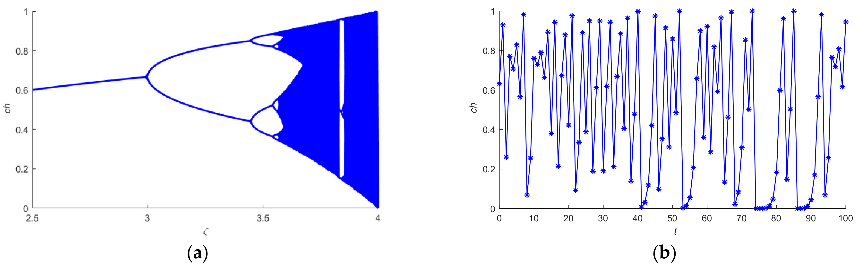
, which is based on the logistic chaotic mapping method according to Equation (11). γ i t is the contraction–expansion coefficient of u i at iteration t according to Equation (2). The values of contraction–expansion coefficient are dynamically updated according to a linear decreasing method for each iteration, and are given by (13) in the following,
γ i t = 0.5 + 1 0.5 t max t t max ,
where t max is the maximum number of iterations. In Equation (12), u o m e a n t is the mean position of the local best for all objects in σ o at iteration t according to Equation (3), and it is given by (14) in the following,
u o m e a n t = 1 n o j = 1 n o u j l b e s t t ,
where u j l b e s t t ( 1 j n o ) is the position of the local best in σ o at iteration t . z i t is the local attractor of u i in σ o at iteration t , which is determined by (15) in the following,
z i t = φ i t u i l b e s t t + 1 φ i t u o g b e s t t ,
where φ i t is regulation parameter at iteration t , and its values are dynamically updated according to Equation (5). u o g b e s t t is the position of the global best for all particles in the population of σ o at iteration t .

4.2.2. The Evolution Rules with Inhibitor

The mechanism of CQPSO is adopted to generate the position of the local attractor and objects in the elementary membrane σ o ( 1 o m ). The evolution rules with inhibitor ¬ p * are of the form: R i = u ¬ p * v . Updating the position for objects in the evolution rules with the inhibitor is determined by Equation (12). A perturbation vector is introduced to the updating method of the local attractor for the objects, which is different from the updating method based on the QPSO technique in the evolution rules with a promoter through Equation (15). The local attractor z i t of object u i in the elementary membrane σ o at iteration t is given by (16) in the following,
z i t = φ i t u i l b e s t t + 1 φ i t u i l b e s t t + Δ i t ,
where u i l b e s t t is the position of the local best for object u i in σ o at iteration t ; note that 1 i i n o . u i is a random object in σ o which is randomly selected from the population of σ o . Δ i t is a perturbation vector, which is determined by (17) according to Equation (9) in the following,
Δ i t = ψ i t u i * l b e s t t u o g b e s t t ,
where ψ i is the adjustment parameter of the local attractor z i , ψ i t = ξ i t t / t max 0.5 . ξ i is a uniform random number of ψ i , which is distributed on the interval from 0 to 1. u i * l b e s t t is the position of the local best for object u i * in σ o at iteration t ; note that 1 i * i i n o , and u i * is a random object which is randomly selected from the population of the elementary membrane σ o .

4.3. Communication Rules

In the proposed CQPSO-ETP, the evolutional antiport rules, as we mentioned above, are introduced to the communication rules to improve the convergence speed and accuracy. The exchange and sharing of information for different membranes or regions is achieved by the execution of the evolutional antiport rules for the objects. Two kinds of communication rules with a promoter/inhibitor are adopted to the CQPSO-ETP, including the communication rules with promoter q * and the communication rules with inhibitor ¬ q * .

4.3.1. The Communication Rules with Promoter

In the CQPSO-ETP, the execution of communication rules with promoter q * depends on the relationship between the elementary membrane σ o and its adjacent membrane o # ; note that 2 o # o m 1 , which are of the form: R o o # = u o g b e s t t q * o u o # g b e s t t o # u r l b e s t t o λ o # , for o # = o 1 or o # = o + 1 . It only can be executed on a moment if there is an elementary membrane σ o in a configuration which contains a multiset of promoter objects, q * . When the communication rule with a promoter is applied, the position u o # g b e s t t of the global best for all objects in the adjacent membrane σ o # of σ o is evolved to the position u r l b e s t t of the local best for a random object, u r , which is randomly selected from the population of σ o , and is send to σ o at iteration t . At the same time, the position u o g b e s t t of the global best for all the objects and promoter object q * in the elementary membrane σ o are consumed during this evolutional antiport process. Especially, if o = 1 , j = m or j = 2 , or else if o = m , j = m 1 or j = 1 .

4.3.2. The Communication Rules with Inhibitor

The execution of communication rules with inhibitor ¬ q * depends on the relationship between the elementary membrane σ o and its adjacent membrane σ o # ; note that 2 o # o m 1 , which are of the form: R o o # = u o g b e s t t ¬ q * o u o # g b e s t t o # λ o u r l b e s t t o # , for o # = o 1 or o # = o + 1 . It only can be executed on a moment if there is an elementary membrane σ o in a configuration which contains a multiset of inhibitor objects ¬ q * . When the communication rule with an inhibitor is applied, the position u o g b e s t t of the global best for all objects in the elementary membrane σ o is evolved to the position u r l b e s t t of the local best for a random object, u r , which is randomly selected from the population of σ o # , and is sent to the adjacent membrane σ o # at iteration t . At the same time, the position u o # g b e s t t of the global best for all objects in the adjacent membrane σ o # and inhibitor object ¬ q * in the elementary membrane σ o are consumed during this evolutional antiport process. Especially, if o = 1 , j = m or j = 2 , or else if o = m , j = m 1 or j = 1 .
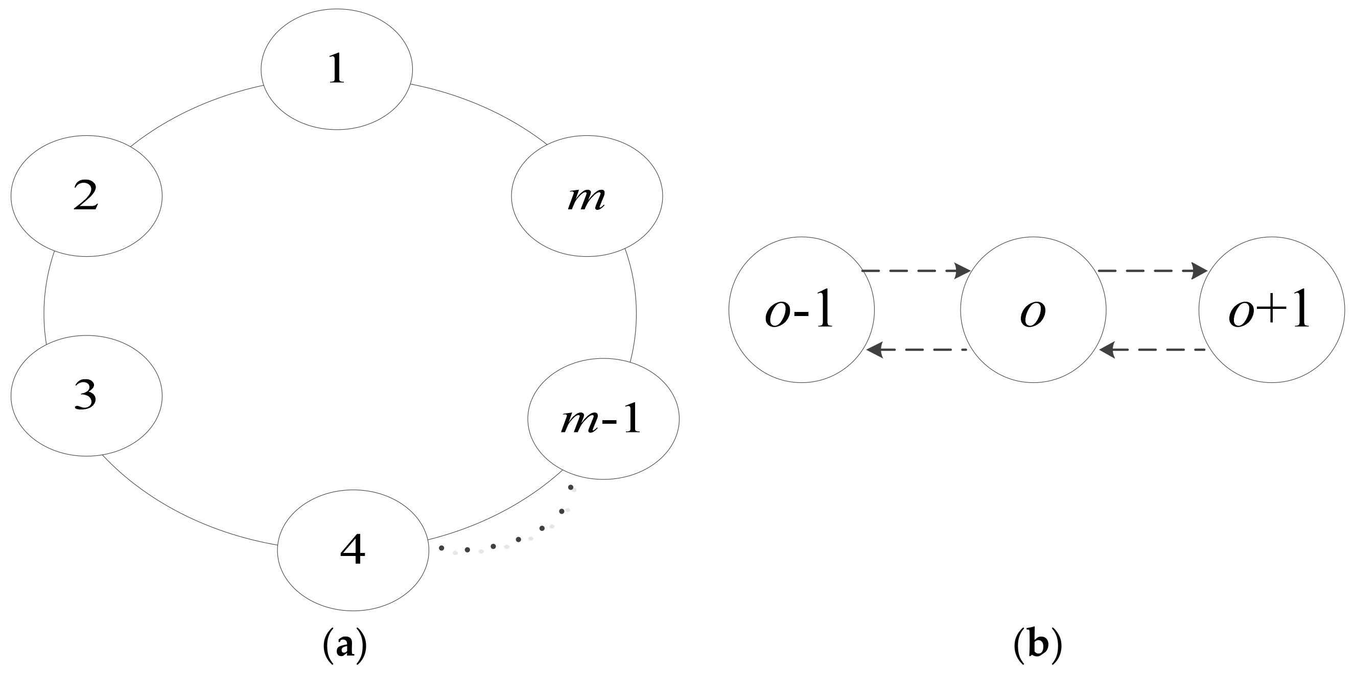
The commutation relationship is established from the execution of communication rules with a promoter/inhibitor between the elementary membrane and its adjacent membrane, which is depicted by a loop topology structure in mathematics, as shown in Figure 3a. Besides this, the communication relationship based on the communication rules with a promoter/inhibitor also constructed the neighborhood structure of the elementary membranes. The exchange and sharing of information only performed on the elementary membrane and its neighboring membranes through communication rules with a promoter/inhibitor, as shown in Figure 3b.
Especially, the communication rules of the elementary membrane σ o ( 1 o m ) and environment σ 0 are also based on the evolutional symport rules for objects, which are of the form: R o 0 = u o g b e s t t o λ 0 λ o u o l b e s t t 0 . When the communication rule is applied, the position u o g b e s t t of the global best for all objects in the elementary membrane σ o is evolved to the position u o l b e s t t of the local best for the object u o , and is sent to the environment σ 0 at iteration t . Then the position u 0 g b e s t t of the global best which is selected from the position u o l b e s t t of the local best for all transformation objects is always stored in the environment as the global best of the system at iteration t .

4.4. Compuatation of CQPSO-ETP

(1)
Initialization
Step1: Parameter initialization
In the proposed CQPSO-ETP, the elementary membrane σ o ( 1 o m ) contains all initial objects, and the number of objects in each membrane is the same, which is denoted by n o as we mentioned above. The total number of objects in this system is denoted by N , where N = o = 1 m n o ;
Step2: Position initialization
The position of the objects is randomly initialized in the search space. The membrane structure of this extended P system is shown in Figure 2. In general, the optimization problem is considered as the minimum optimization problem;
Step3: Update the position of the local best and global best
Update the position of the local best and global best for all objects in each elementary membrane. Note that the promoter and inhibitor will not simultaneously exist in the same elementary membrane. The evolution and communication rules with the promoter/inhibitor are only executed on a configuration at a moment when the promoter/inhibitor objects have appeared in the elementary membrane.
(2)
Evolution rules for objects
The promoter p * and inhibitor ¬ p * in the evolution rules are described as some restricted conditions of the system, including the comparison condition and stagnation condition. The comparison condition is adopted to compare the fitness values of the global best in the elementary membrane and its neighboring membranes, and the stagnation condition is adopted to evaluate whether the position of the global best for all objects in the elementary membrane cannot be further improved for l i m i t iterations.
Step1: if p * = f u o g b e s t f u o # g b e s t l i m i t 2 , for 1 o o # m , the evolution rules with promoter p * for the objects are adopted to update the position of the local best and global best in each elementary membrane, according to Equations (12)–(15); if ¬ p * = f u o g b e s t > f u o # g b e s t l i m i t > 2 , for 1 o o # m , the evolution rules with inhibitor ¬ p * for the objects are adopted to update the position of the local best and global best in each elementary membrane, according to Equations (12)–(14), (16) and (17);
Step2: Update the position of the local best and global best in each elementary membrane.
(3)
Communication rules for objects
The promoter q * and inhibitor ¬ q * in the communication rules are considered as some comparison conditions. The comparison condition is introduced to compare the fitness values of the global best for all objects in the elementary membrane and its neighboring membranes.
Step1: if q * = f u o g b e s t > f u o # g b e s t , for 1 o o # m , the evolutional antiport rules with promoter q * are adopted to transport the position of the global best in the neighboring membrane to the elementary membrane; if ¬ q * = f u o g b e s t f u o # g b e s t , for 1 o o # m , the evolutional antiport rules with inhibitor ¬ q * are adopted to transport the position of the global best in the elementary membrane to its neighboring membranes;
Step2: The position u o g b e s t of the global best for object u o in each elementary membrane is sent to the environment through the execution of communication rules, R o 0 , and is evolved to the position u o l b e s t of the local best for object u o in the environment. Then the environment stored the best position among these transformation local bests as the global best in the system, and it also represented the computational results of the system for each iteration.
(4)
Halting and output
The evolution and communication rules for objects in the proposed CQPSO-ETP will be implemented repeatedly with an iterative form until the termination criterion is satisfied. The termination criterion of CQPSO-ETP is stopped when the maximum number of iterations is reached. When the system halts, the position of the last global best, which is stored in the environment, is regarded as the final computational results for the system. Algorithm 1 depicted the main pseudo code of the computation for proposed CQPSO-ETP.
Algorithms1 CQPSO-ETP: The pseudo code of computation.
Input: n o , m , t max , c 1 , c 2 , r 1 , r 2 , φ , η , γ , ζ , ψ , N ;
    (1) Initialization
      Update the local and global best;
                for   o = 1 to m
    for i = 1 to n o , n o = N / m
       u i l b e s t = object(i). Local best. Position;
       f u i l b e s t = object(i). Local best. Fitness;
      if u i l b e s t < u o g b e s t
        u o g b e s t = object(i). Global best. Position;
        f u o g b e s t = object(i). Global best. Fitness;
      end if
    end
   end
for t = 1 to t max
    (2) Evolution rules for objects
      for o = 1 to m
    for i = 1 to n o
      Step 1: if p * = f u o g b e s t f u o # g b e s t l i m i t 2 , o o #
         z i t = φ i t u i l b e s t t + 1 φ i t u o g b e s t t ;
         u i t + 1 = z i t ± γ i t u o m e a n t u i t ln 1 / η i t ;
        else ¬ p * = f u o g b e s t > f u o # g b e s t l i m i t > 2 , o o #
            z i t = φ i t u i l b e s t t + 1 φ i t u i l b e s t t + Δ i t ;
            u i t + 1 = z i t ± γ i t u o m e a n t u i t ln 1 / η i t ;
        end
      Step2: update the local and global best;
 end
   end
(3) Communication rules for the objects
      for o = 1 to m
    Step 1: if q * = f u o g b e s t > f u o # g b e s t , o o #
R o o # = u o g b e s t t q * o u o # g b e s t t o # u r l b e s t t o λ o # , o # = o 1 , o # = o + 1 ;
else ¬ q * = f u o g b e s t f u o # g b e s t , o o #
R o o # = u o g b e s t t ¬ q * o u o # g b e s t t o # λ o u r l b e s t t o # , o # = o 1 , o # = o + 1
      end
Step 2: R o 0 = u o g b e s t t o λ 0 λ o u o l b e s t t 0 ;
      Update the global best in the system
end
end
(4) Halting and output
      if t > t max
    u 0 g b e s t t =Best Position;
    f u 0 g b e s t t =Best Fitness;
      end
Output: Best Position, Best Fitness.

4.5. Complexity Analysis

The complexity of the proposed CQPSO-ETP is analyzed in this subsection. As defined earlier, N is the total number of objects in the system. n o ( 1 o m ) is the initial number of objects in the elementary membrane σ o , where N = n o m . m is the number of the elementary membranes in the system. t max is the maximum number of iterations. D is the dimension of the search space. The computation of the proposed CQPSO-ETP consists of three steps. In the first step of initialization, the computational time of fitness function for the initial objects in each elementary membrane is n o D . Due to the parallel working manner, the complexity of the initialization for the system is O n o D . In the second step, the computational time for the execution of the evolution rules with a promoter for the objects is the same as the computational time for the execution of the evolution rules with an inhibitor for the objects. Moreover, the computing time needed by executing one evolution rule with a promoter or inhibitor for an object is D . Hence, the total computing time needed by executing one evolution rule with a promoter/inhibitor for the objects in each elementary membrane is n o D . Therefore, the complexity of the evolution process for all objects in the system is O n o D . In the third step, the communication time for the execution of the communication rules with a promoter is same as the communication time for the execution of the communication rules with an inhibitor, which contains the exchange time for objects between the membrane and its neighboring membranes. The communication time needed by executing one communication rule is 2. Therefore, the complexity of the communication process for all elementary membranes in the system is O 2 . As a result, the computational time at each iteration for the system is n o D + 2 . Thus, the total computational time needed for the computing process of CQPSO-ETP is n o D + t max n o D + 2 , and the complexity of the system is O n o D + t max n o D + 2 . As the number of objects in each elementary membrane is the same and will not change in the computing process, which is denoted by n , then n = n o = N / m . The complexity of the proposed CQPSO-ETP is also described as O n D + t max n D + 2 , which can be simplified to O t max n D .

5. Experimental Results and Analysis

Computational experiments which are made on some classic numerical benchmark functions are conducted to verify the optimization performance of the proposed CQPSO-ETP. More details about eight classic numerical benchmark functions which are used in this computational experiment are given in this section. Furthermore, the optimized efficiency of CQPSO-ETP is compared with classic PSO, QPSO and two existing improved QPSO approaches in the comparison experiment. All optimized techniques, including CQPSO-ETP, are implemented on MATLAB (2016b) and all experiments are conducted on a DELL desktop computer with an Intel 8.00 GHz i7-8550U processor and 16 GB of RAM in a Windows 10 Environment.

5.1. Numerical Benchmark Functions

In this work, eight classic numerical benchmark functions from the previous work, which are reported in [102], are adopted to the computational experiments, including unimodal and multimodal functions. Unimodal and multimodal functions are usually used to evaluate the exploitation and exploration efficiency of optimized approaches.
The domains and minimums of eight classic numerical benchmark functions are depicted in Table 1, including the Rastrigin function, the Sum power function, the Alpine function, the Schwefel 1.2 function, the Rosenbrock function, the Sum Squares function, the Quartic function, and the Schwefel function. Additionally, the dimension of the eight benchmark functions which are used in the computational experiment is set to 2 and 10 in order to get more meaningful results. The shape and range of eight classic numerical benchmark functions for D = 2 are depicted in Figure 4.

5.2. Comparision with Other Optimized Approaches

The optimized efficiency of the proposed CQPSO-ETP is compared with the classic PSO, QPSO and two improved QPSO approaches, i.e., sequential synchronous quantum-behaved particle swarm optimization (SAQPSO) [103] and improved quantum-behaved particle swarm optimization based on adaptive behavior selection (AQPSO) [93] as described above, which have been reported in the previous literature. The population of particles in the SAQPSO are divided into multiple sub-populations, and the global best in each sub-population is adopted to the commutation information with the others. A diversity function is introduced to the update of the acceleration factors which are based on the proximity between the current position and the global best for each particle in the AQPSO. The values of the adjustable parameters in the comparative techniques are the best ones which have been reported in the respective references, as listed in Table 2.
The proposed CQPSO-ETP and other compared approaches were also run 50 independent times to eliminate the effects of random factors. Simple statistics, including worst values (Worst), best values (Best), mean values (Mean) and standard deviations (S.D.), of fitness function are adopted to the computational experiment as the evaluation criterion to measure the effectiveness of these optimized techniques. Figure 5 shows the convergence results of these comparative techniques on eight numerical benchmark functions from f 1 x to f 8 x with D = 2 .
Compared with classic PSO, QPSO and AQPSO, the fitness values of the proposed CQPSO-ETP declined quickly at the beginning of the evolutionary process from Figure 5a–d,f, and the slope of the convergence curve obtained by the proposed CQPSO-ETP is the maximum, compared with other optimization techniques. It means that the proposed CQPSO-ETP has small fitness values among comparative techniques on the eight numerical benchmark functions, as shown in Figure 5. To be more clear, the experimental results of the proposed CQPSO-ETP and other compared approaches, which are made on eight classic numerical benchmark functions, are reported in Table 3.
The difference of comparison results obtained by optimized techniques is obvious, as indicated by Table 3, and the statistical results obtained by CQPSO−ETP, including Mean and S.D., which are the minimum among the comparison results. Therefore, the proposed CQPSO−ETP has a better performance than classic PSO, QPSO, SAQPSO and AQPSO on most of the classic numerical benchmark functions with D = 2 . The mean of the computational time which is taken by the comparative techniques is given in Table 4, thus the computational time of CQPSO−ETP is acceptable compared with other optimized techniques.
Furthermore, Figure 6 gives the convergence of these optimized techniques on eight numerical benchmark functions from f 1 x to f 8 x with the dimension of the search space being 10, D = 10 . Simple statistics of fitness function obtained by the optimized techniques are reported in Table 5, including the worst values (Worst), best values (Best), mean values (Mean) and standard deviations (S.D.). In general, the experimental result shows that the proposed CQPSO−ETP has a better performance than other optimization techniques, like classic PSO, QPSO, SAQPSO and AQPSO, both in classic unimodal and multimodal functions with D = 2 and D = 10 .

5.3. Firedman Test Statistic

The Friedman test is introduced in the comparison experiment to investigate the difference of these optimized techniques, and the average value of the fitness function obtained by the comparative techniques is used to the evaluation criterion of Friedman test. The null hypothesis of the Friedman statistic test is that all optimized techniques in this experiment have the same performance for any one benchmark function with D = 2 and D = 10 . Mathematically, the Friedman test works as follows [104].
In the Friedman test, the average of the fitness values of the comparative techniques of the eight benchmark functions are ranked from the smallest to largest [105]. Moreover, the rank of comparative technique j on benchmark function i is denoted by r i j , for j = 1 , 2 , , 5 , i = 1 , 2 , , 8 , where j and i are the labels of the comparative approach and benchmark function. The average of these ranks is denoted by 1 2 p + 1 , in case 3, where p is the total number of the optimized techniques in the comparison experiments, in case 5. The Friedman test statistic χ r 2 is given by (18) in the following
χ r 2 = 12 n p ( p + 1 ) p = 1 p ( i = 1 n r i j ) 2 3 n ( p + 1 ) ,
where n is the total number of the benchmark functions in the experiment, for n = 8 . The Friedman test statistic follows a Chi−squared distribution with p 1 degrees of freedom.
Table 6 and Table 7 present the ranks of fitness values obtained by these optimized approaches for each numerical benchmark function with D = 2 and D = 10 . The proposed CQPSO−ETP is ranked highest for each benchmark functions with D = 2 and D = 10 . With p 1 = 4 degrees of freedom, the critical value of the statistic which is denoted by χ at the significance level α = 0.05 is 9.448, where χ = 9.448 . The Friedman test statistics χ r 2 in the comparison experiment with D = 2 and D = 10 , are computed using the ranks from Table 6 and Table 7, and the results of χ r 2 are: for D = 2 , χ r 2 = 25.95 ; for D = 10 , χ r 2 = 23.55 . Hence, due to χ r 2 = 25.95 > χ 2 = 9.488 with D = 2 , and χ r 2 = 23.55 > χ 2 = 9.488 with D = 10 , the conclusions of the Friedman test are to reject the null hypothesis, i.e., the performance of the comparative techniques level is significantly different. It was, in this comparison experiment, the optimized techniques which obtained a significantly different performance through the values of fitness function on the eight classic numerical benchmark functions with D = 2 and D = 10 .

6. The Proposed CQPSO−ETP for Image Segmentation Problems

In this section, experiments which are made on image segmentation problems with different tested images are performed, and the comparison results obtained by different classic clustering approaches, including CQPSO−ETP, are reported and discussed in order to validate the clustering efficiency of the proposed CQPSO−ETP. Eight tested images from the classic image segmentation datasets are used in the comparison experiments. All comparative clustering approaches are implemented on MATLAB (2016b), and all experiments are conducted on a DELL desktop computer with an Intel 8.00 GHz i7−8550U processor and 16 GB of RAM in a Windows 10 Environment.

6.1. Tested Images

Eight tested images are used in the comparison experiment, including a Swan, Aircraft, Eagle, Goshawk, Plane, White Bear, Daisy and Parrot, from the previous studies and researches about the Berkeley Segmentation Dataset and Benchmark [106]. The size of the tested image is set to 481*321. More details about these tested images are given in Figure 7, and the label information about these tested images using the grey region are given in Figure 8. As is graphically depicted in Figure 8, the number of the classes of the Swan image, Aircraft image and Eagle image are set to 2, the number of the classes of the Goshawk image and Plane image are set to 3, the number of the classes of the White Bear image and Daisy image are set to 5, and the number of the classes of the Parrot image is set to 7.

6.2. Evaluation Funcion

As we mentioned above, the position of the i -th object in the proposed CQPSO−ETP can be viewed as the potential solution in the search space for the optimization problems. Therefore, in the image segmentation problems, the position of the i -th object u i can be regarded as a partitioning of an image, which is represented by a set of cluster centers, u i t = c i 1 , c i 2 , , c i K , for 1 t t max , where K is the number of the clusters or classes in an image, and c i j ( 1 j K ) represents cluster center j in the position of object i . The classification of a pixel is correct or accurate if it is clustered into the right cluster or class [107]. Therefore, the classification rate, also called clustering accuracy, is denoted by A . The clustering accuracy of an image is defined to the proportional correctly classified pixels in an image, as shown in (19) in the following,
A = 1 G i = 1 K max j K D i R j ,
where D = D 1 , D 2 , , D K is the partitioning results of an image obtained by clustering techniques, and D j ( 1 j K ) represents the j -th cluster. R = R 1 , R 2 , , R K is the real partition of an image, and R j ( 1 j K ) represents the j -th real cluster. max j K D i R j is the total number of correctly classified pixels, and G is the total number of pixels in an image. In this work, the clustering accuracy A is also used to evaluate the clustering performance of these comparative clustering techniques.

6.3. Comparision Results

Superpixel segmentation is an important image preprocessing technique, reported in the previous work, which groups pixels into many perceptually meaningful regions on the atomic level, rather than the traditional rigid structure of the pixel in the image. A lot of researches and works about superpixel segmentation approaches have been reported, and both of them have their own particular application. In this work, a classic superpixel technique, named simply as linear iterative clustering (SLIC) [108], is introduced to the preprocessing of the tested images in order to simplify the clustering data for the comparative clustering techniques. The SLIC based on a K−means clustering technique is used to generate superpixels based on the similarity of pixels through a linear iterative manner. The number of superpixels is usually set to 200 for the tested images. The achievable segmentation results based on the SLIC technique on eight tested images are shown in Figure 9.
The clustering performance of the proposed CQPSO−ETP is compared with three classic clustering techniques, including K−means, Spectral clustering (SC) and PSO, and the intra−cluster compactness as the fitness function of the PSO and the proposed CQPSO−ETP. The comparison experiments which are made on the segmentation results based on the SLIC technique are conducted to verify the clustering efficiency of the proposed CQPSO−ETP. These comparative clustering approaches were run for 50 independent times for each tested image so as to get some meaningful clustering results and eliminate the effects of random factors.
The segmentation results obtained by these comparative clustering approaches on the eight tested images are shown in Figure 10. The boundary and regions of the segmentation image obtained by the proposed CQPSO−ETP are more clear than others. Furthermore, Table 8 gives the statistic results of clustering accuracy A from these comparative clustering approaches on the tested images, including Worst, Best, Mean and S.D. The computing results on the eight tested images are shown in Table 8. The proposed CQPSO−ETP has better a clustering performance than the other three classic clustering techniques on the tested images, especially in the mean results of the fitness function.
The mean of the computational time obtained by these comparative clustering techniques is given in Table 9, and the computational time of the proposed CQPSO−ETP is acceptably compared with the other clustering techniques. Lastly, the Friedman test is also applied to the Means of the clustering accuracy in this comparison experiment in order to prove the difference between the proposed CQPSO−ETP and other comparative techniques. The ranks of the clustering accuracy obtained by the comparative clustering approaches for each tested image are presented in Table 10. With p 1 = 3 degrees of freedom, the critical value is χ 2 = 7.815 at the significance level α = 0.05 [104]. The computed Friedman test statistic is χ r 2 = 18.225 through Table 10, where χ r 2 = 18.225 > χ 2 = 7.815 . Therefore, these comparative clustering approaches obtained significantly different clustering accuracies in this comparison experiment [105].

7. Conclusions

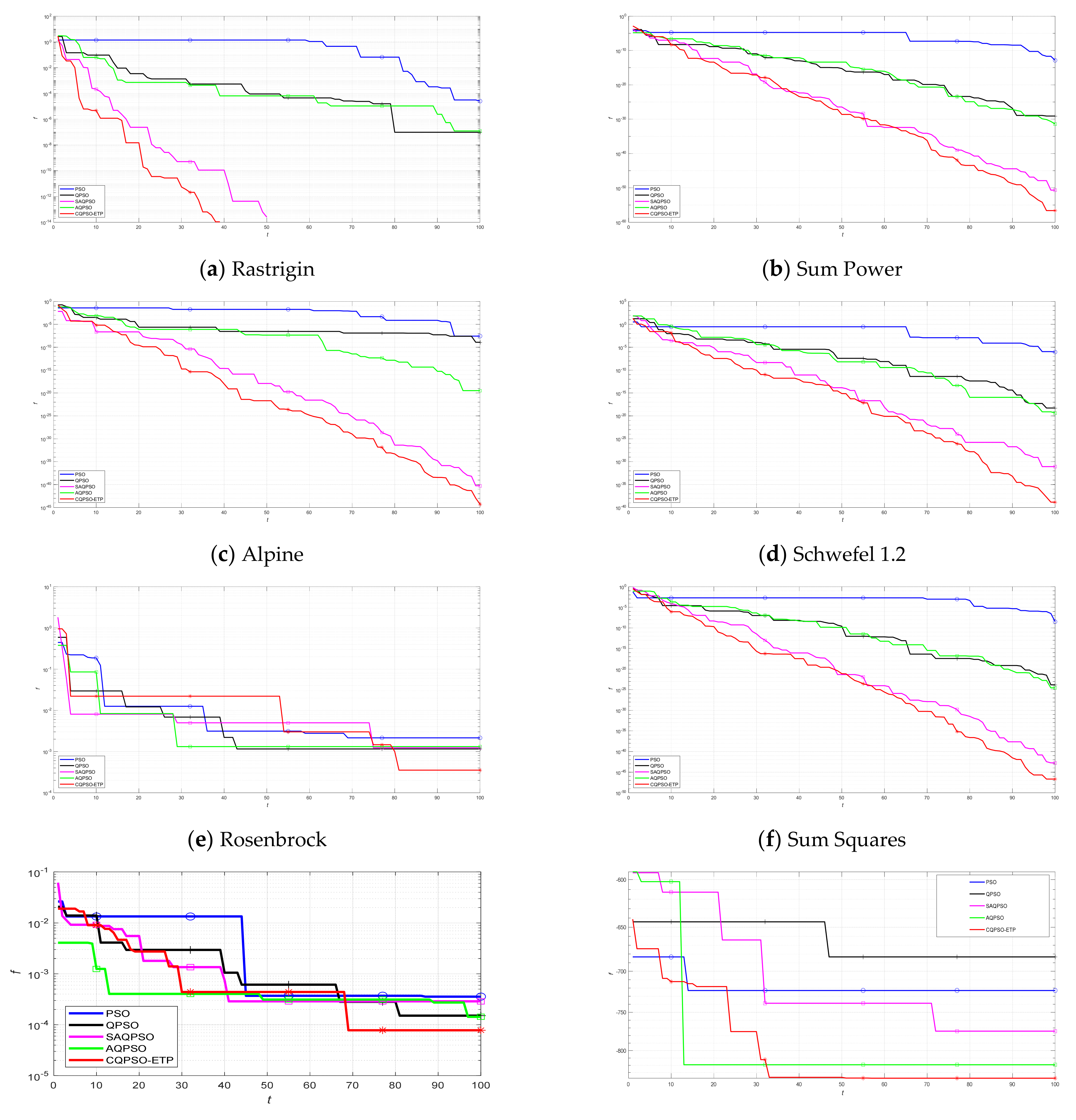
An extended tissue−like P system combining the evolutionary mechanism of QPSO and improved QPSO and the evolution–communication mechanism of tissue−like P systems is proposed, called the CQPSO−ETP, to solve optimization problems and image segmentation problems. This extended tissue−like P system under the framework of membrane computing using the tissue−like P system with evolutional symport/antiport rules and a promoter/inhibitor for objects, and the distributed parallel computing model of tissue−like P systems is adopted to enhance the global search ability of the CQPSO−ETP. Different from the existing SNS−based MIEAs, the CQPSO−ETP has two kinds of evolution rules with a promoter and inhibitor for objects. The evolution rules with a promoter are based on the basic position updating strategy for particles in a standard QPSO. Other evolution rules with an inhibitor are based on the position updating strategy for particles in an improved QPSO using self−adaptive selection, and cooperative evolutionary and logistic chaotic mapping methods, to accomplish the evolution of the objects in the system. The evolution mechanism for objects based on the QPSO and improved QPSO is used to improve the optimization performance of the CQPSO−ETP. The communication rules with promoter and inhibitor for objects are adopted to transfer the local and global best positions of objects to achieve the exchange and sharing of information between different membranes. The communication mechanism for objects based on communication rules in tissue−like P systems is introduced to improve the convergence speed and accuracy. The promoter and inhibitor are also introduced to control the exchanged direction of information between different membranes. The computational experiments, which are compared with PSO, QPSO and two improved QPSO approaches, are evaluated on eight classic numerical benchmark functions from previous studies and researches, and the results clearly exhibit the optimization effectiveness of this proposed extended tissue−like P system. Furthermore, the comparison experiments which are made on eight tested images from the image segmentation datasets are conducted to verify the clustering performance of the CQPSO−ETP as compared with three classic clustering techniques, including K−means, SC, and PSO, and the computational results show the validity of this extended tissue−like P system.
The computing model of tissue−like P systems is the parallel computing model, which is highly effective and more efficient in solving optimization problems with linear or polynomial complexity. However, the application of tissue−like P systems has been limited by the incomplete fundamental operation and implementation difficulties. The evolution mechanism based on the evolution computing techniques provides a new way to achieve the evolutionary process for objects in P systems. Then, the computation of tissue−like P systems in biology, which contain the execution of the evolution and communication rules for objects, is converted to the update and exchange of potential solutions in mathematics. The proposed CQPSO−ETP takes the tissue−like P system with evolutional symport/antiport rules and a promoter/inhibitor as the basic computational structure, and the communication rules for objects will establish the communication relationship between different membranes and regions in P systems. These relation links between different membranes and regions are bidirectional, which are simple and easy to implement. However, these static relation links in future studies are going to be replaced by dynamic relation links in order to further accelerate convergence and improve the population diversity. Besides, a more complicated membrane computing structure in P systems may be introduced in future studies to improve the optimization performance of the SNS−based MIEAs. Furthermore, the computing experiments were only executed on a low dimensional search space for classic numerical benchmark functions, and the proposed CQPSO−ETP may have some limitations in a high dimensional space. Therefore, future studies may test the effectiveness of CQPSO−ETP using high dimensional benchmark functions, and may also focus on MIEAs based on the extended neural−like P systems and other bio−inspired computing models. More works are also needed to balance the local and global search abilities of this proposed extended P system.

Author Contributions

Validation and writing, L.W.; conceptualization, X.L.; formal analysis, J.Q.; investigation, Y.Z.; data curation, Z.J.; supervision, N.W. All authors have read and agreed to the published version of the manuscript.

Funding

This research received no external funding.

Institutional Review Board Statement

Not applicable.

Informed Consent Statement

Not applicable.

Data Availability Statement

The eight tested images are from the Berkely computer vision group, Berkely segmentation dataset, and benchmark (BSDS300), available at: https://www2.eecs.berkeley.edu/Research/Projects/CS/vision/grouping/segbench/ (accessed on: 1 October 2020).

Acknowledgments

This research project was partially supported by the Doctor Foundation of Shandong Jianzhu University (X21008Z, XNBS20119), the National Natural Science Foundation of China (61876101, 61802234, 61806114), the National Natural Science Foundation of the Shandong Province, China (ZR2019QF007), the Ministry of Education Humanities and Social Science Research Youth Foundation, China (19YJCZH244), the Social Science Fund Project of the Shandong Province, China (16BGLJ06, 11CGLJ22), the Special Postdoctoral Project of China (2019T120607), the Postdoctoral Project of China (2017M612339, 2018M642695).

Conflicts of Interest

The authors declare that there is no conflict of interest regarding the publication of this paper.

References

  1. Păun, G. Membrane computing: An introduction. Theor. Comput. Sci. 2002, 287, 73–100. [Google Scholar] [CrossRef] [Green Version]
  2. Păun, G. Membrane computing and economics: A General View. International journal of computers. Commun. Control 2016, 11, 105–112. [Google Scholar]
  3. Pan, L.; Zeng, X.; Song, T. Membrane Computing an Introduction, 1st ed.; Huazhong University of Science and Technology Press: Wuhan, China, 2012; pp. 1–10. [Google Scholar]
  4. Păun, G. A dozen of research topics in membrane computing. Theor. Comput. Sci. 2018, 736, 76–78. [Google Scholar] [CrossRef]
  5. Li, B.; Peng, H.; Wang, J. A novel fusion method based on dynamic threshold neural P systems and nonsubsampled contourlet transform for multi−modality medical images. Signal Processing 2021, 178, 35–59. [Google Scholar] [CrossRef]
  6. Song, B.; Pan, L.; Zhang, C. Tissue−like P systems with evolutional symport/antiport rules. Inf. Sci. 2017, 378, 177–193. [Google Scholar] [CrossRef]
  7. Martín, D.; Cabrera, L.; Núez, A.; Jiménez, M. Membrane creation in polarizationless P systems with active membranes. Fundam. Inform. 2019, 171, 297–311. [Google Scholar] [CrossRef]
  8. Pan, L.; Martín, D.; Song, B.; Jiménez, M. Cell−like P systems with polarizations and minimal rules. Theor. Comput. Sci. 2020, 816, 1–18. [Google Scholar] [CrossRef]
  9. Jin, Y.; Song, B.; Li, Y. Time−free solution to independent set problem using P systems with active membranes. Fundam. Inform. 2021, 182, 243–255. [Google Scholar] [CrossRef]
  10. Song, B.; Li, K.; Martín, D.; Cabrera, L.; Jiménez, M. Cell−like P systems with evolutional symport/antiport rules and membrane creation. Inf. Comput. 2020, 275, 104542. [Google Scholar] [CrossRef]
  11. Martín, D.; Amora, D.; Cabrera, L.; Song, B.; Pan, L.; Mario, J. P systems with symport/antiport rules: When do the surroundings matter. Theor. Comput. Sci. 2020, 805, 206–217. [Google Scholar] [CrossRef]
  12. Pan, L.; Alhazov, A.; Su, H.; Song, B. Local synchronization on asynchronous tissue P systems with symport/antiport rules. IEEE Trans. NanoBioscience 2020, 19, 315–320. [Google Scholar] [CrossRef] [PubMed]
  13. Martín, D.; Cabrera, L.; Mario, J. P systems with evolutional communication and division rules. Axioms 2021, 10, 1–17. [Google Scholar]
  14. Song, B.; Pan, L. The computational power of tissue−like P systems with promoters. Theor. Comput. Sci. 2016, 641, 43–52. [Google Scholar] [CrossRef]
  15. Song, B.; Zeng, X.; Jiang, M.; Jiménez, M. Monodirectional tissue P systems with promoters. IEEE Trans. Cybern. 2021, 51, 438–450. [Google Scholar] [CrossRef] [PubMed]
  16. Song, B.; Li, K.; Zeng, X. Monodirectional evolutional symport tissue P systems with promoters and cell division. IEEE Trans. Parallel Distrib. Syst. 2022, 33, 332–342. [Google Scholar] [CrossRef]
  17. Luo, Y.; Zhao, Y.; Chen, C. Homeostasis tissue−like P systems. IEEE Trans. Nanobioscience 2021, 20, 126–136. [Google Scholar] [CrossRef]
  18. Luo, Y.; Guo, P.; Jiang, Y.; Zhang, Y. Timed homeostasis tissue−like P systems with evolutional symport/antiport rules. IEEE Access 2020, 8, 131414–131424. [Google Scholar] [CrossRef]
  19. Fan, S.; Paul, P.; Wu, T.; Rong, H.; Zhang, G. On applications of spiking neural P systems. Appl. Sci. 2020, 10, 7011. [Google Scholar] [CrossRef]
  20. Song, X.; Cabrera, L.; Peng, H.; Wang, J.; Jiménez, M. Spiking neural P systems with delay on synapses. Int. J. Neural Syst. 2020, 31, 2050042. [Google Scholar] [CrossRef]
  21. Yin, X.; Liu, X. Dynamic threshold neural P systems with multiple channels and inhibitory rules. Processes 2020, 8, 1281. [Google Scholar] [CrossRef]
  22. Ren, Q.; Liu, X.; Sun, M. Turing universality of weighted spiking neural P systems with anti−spikes. Comput. Intell. Neurosci. 2020, 2020, 8892240. [Google Scholar] [CrossRef] [PubMed]
  23. Peng, H.; Li, B.; Wang, J.; Song, X.; Jiménez, M. Spiking neural P systems with inhibitory rules. Knowl.−Based Syst. 2020, 188, 105064. [Google Scholar] [CrossRef]
  24. Song, B.; Li, K.; Matín, D.; Mario, J. A survey of nature−inspired computing: Membrane computing. ACM Comput. Surv. 2021, 54, 2201–2231. [Google Scholar] [CrossRef]
  25. Boussa, I.; Lepagnot, J.; Siarry, P. A survey on optimization metaheuristics. Inf. Sci. 2013, 237, 82–117. [Google Scholar] [CrossRef]
  26. Bagchi, P.; Pal, S. Controlling crossover probability in case of a genetic algorithm. Commun. Comput. Inf. Sci. 2011, 147, 287–290. [Google Scholar]
  27. Zhang, G.; Jiménez, M.; Gheorghe, M. Real−Life Applications with Membrane Computing, 1st ed.; Springer Press: Berlin/Heidelberg, Germany, 2017; pp. 11–12. [Google Scholar]
  28. Holland, J. Adaptation in Natural and Artificial Systems, 1st ed.; MIT Press: Cambridge, UK, 1992; pp. 201–205. [Google Scholar]
  29. Rechenberg, I. Evolutions strategie: Optimierung technischer systemenach prinzipiender biologischen evolution. Stuttg.−Holzboog 1973, 1, 1–18. [Google Scholar]
  30. Fogel, L.; Owens, A.; Walsh, M. Artificial Intelligence through Simulated Evolution, 1st ed.; Wiley−IEEE Press: London, UK, 1966; pp. 160–170. [Google Scholar]
  31. Koza, J. Genetic Programming: On the Programming of Computers by Means of Natural Selection, 1st ed.; MIT Press: Cambridge, UK, 1992; pp. 619–623. [Google Scholar]
  32. Han, K.; Kim, J. Quantum−inspired evolutionary algorithm for a class of combinatorial optimization. IEEE Trans. Evol. Comput. 2002, 6, 580–593. [Google Scholar] [CrossRef] [Green Version]
  33. Cerný, V. Thermodynamical approach to the traveling salesman problem: An efficient simulation algorithm. J. Optim. Theory Appl. 1985, 45, 41–51. [Google Scholar] [CrossRef]
  34. Das, S.; Suganthan, P. Differential evolution: A survey of the state−of−the−art. IEEE Trans. Evol. Comput. 2011, 15, 4–31. [Google Scholar] [CrossRef]
  35. Glover, F. Tabu search−part I. INFORMS J. Comput. 1989, 1, 190–206. [Google Scholar] [CrossRef] [Green Version]
  36. Kennedy, J.; Eberhart, R. Particle swarm optimization. In Proceedings of the IEEE International Conference on Neural Networks, Perth, Australia, 27 November–1 December 1995; pp. 69–73. [Google Scholar]
  37. Dorigo, M.; Birattari, M.; Stutzle, T. Ant colony optimization. IEEE Comput. Intell. Mag. 2006, 1, 28–39. [Google Scholar] [CrossRef]
  38. Karaboga, D. An Idea Based on Honey Bee Swarm for Numerical Optimization; Technical Report−TR06; Erciyes University, Engineering Faculty, Computer Engineering Department: Kayseri, Turkey, 2005; pp. 1–10. [Google Scholar]
  39. Simon, D. Biogeography−based optimization. IEEE Trans. Evol. Comput. 2008, 12, 702–713. [Google Scholar] [CrossRef] [Green Version]
  40. Li, L.; Shao, Z.; Qian, J. An optimizing method based on autonomous animate: Fish swarm algorithm. System Engineering−Theory and Practice 2002, 11, 32–38. [Google Scholar]
  41. Eiben, A.; Smith, J. Introduction to Evolutionary Computing, 1st ed.; Springer Press: Berlin/Heidelberg, Germany, 2003; pp. 13–24. [Google Scholar]
  42. Deb, K.; Mohan, M.; Mishra, S. Evaluating the−domination based multi−objective evolutionary algorithm for a quick computation of Pareto−optimal solutions. Evol. Comput. 2005, 13, 501–525. [Google Scholar] [CrossRef]
  43. Zhang, G.; Gheorghe, M.; Pan, L.; Jiménez, M. Evolutionary membrane computing: A comprehensive survey and new results. Inf. Sci. 2014, 279, 528–551. [Google Scholar] [CrossRef]
  44. Zhao, Y.; Liu, X.; Sun, M.; Qu, J.; Zheng, Y. Time−free cell−like P systems with multiple promoters/inhibitors. Theor. Comput. Sci. 2020, 843, 73–83. [Google Scholar] [CrossRef]
  45. Păun, G.; Rozenberg, G.; Salomaa, A. The Oxford Handbook of Membrane Computing, 1st ed.; Oxford University Press: New York, NY, USA, 2010; pp. 310–332. [Google Scholar]
  46. Chen, G.; Hu, J.; Peng, H.; Wang, J.; Huang, X. A spectral clustering algorithm improved by P systems. Int. J. Comput. Commun. Control 2018, 13, 759–771. [Google Scholar] [CrossRef]
  47. Liu, C.; Du, Y.; Li, A.; Lei, J. Evolutionary multi−objective membrane algorithm. IEEE Access 2019, 8, 6020–6031. [Google Scholar] [CrossRef]
  48. He, J.; Xiao, J.; Liu, X. A novel membrane−inspired algorithm for optimizing solid waste transportation. Optik 2015, 126, 3883–3888. [Google Scholar] [CrossRef]
  49. Huang, L.; Suh, I.; Abraham, A. Dynamic multi−objective optimization based on membrane computing for control of time−varying unstable plants. Inf. Sci. 2011, 181, 2370–2391. [Google Scholar] [CrossRef]
  50. Wang, L.; Liu, X.; Sun, M.; Qu, J. An extended clustering membrane system based on particle swarm optimization and cell−like P system with active membranes. Math. Probl. Eng. 2020, 2020, 5097589. [Google Scholar] [CrossRef] [Green Version]
  51. Wang, Y.; Liu, X.; Xiang, L. GA–based membrane evolutionary algorithm for ensemble clustering. Comput. Intell. Neurosci. 2017, 2017, 4367342. [Google Scholar] [CrossRef] [PubMed] [Green Version]
  52. Peng, H.; Wang, J.; Jiménez, M.; Núnez, A. An unsupervised learning algorithm for membrane computing. Inf. Sci. 2015, 304, 80–91. [Google Scholar] [CrossRef]
  53. Wang, J.; Peng, H.; Yang, J.; Huang, X.; Zhang, J. DE−MC: A membrane clustering algorithm based on differential evolution mechanism. Rom. J. Inf. Sci. Technol. 2014, 17, 77–89. [Google Scholar]
  54. Guo, P.; Hou, M.; Ye, L. MEATSP: A membrane evolutionary algorithm for solving TSP. IEEE Access 2020, 8, 199081–199096. [Google Scholar] [CrossRef]
  55. Zhao, Y.; Zhang, W.; Sun, M.; Liu, X. An improved consensus clustering algorithm based on cell−like P systems with multi−catalysts. IEEE Access 2020, 8, 154502–154517. [Google Scholar] [CrossRef]
  56. Wang, H.; Chen, S.; Luo, L. A diffusion algorithm based on P systems for continuous global optimization. J. Comput. Sci. 2020, 44, 101112. [Google Scholar] [CrossRef]
  57. Rosas, U.; Montiel, O.; Sepúlveda, R. Mobile robot path planning using membrane evolutionary artificial potential field. Appl. Soft Comput. 2019, 77, 36–251. [Google Scholar]
  58. Cheng, J.; Zhang, G.; Zeng, X. A novel membrane algorithm based on differential evolution for numerical optimization. Int. J. Unconv. Comput. 2011, 7, 159–183. [Google Scholar]
  59. Guo, D.; Zhang, G.; Zhou, Y.; Yuan, J.; Paul, P.; Fu, K.; Zhu, M. Image thresholding using a membrane algorithm based on enhanced particle swarm optimization with hyperparameter. Int. J. Unconv. Comput. 2020, 15, 63–106. [Google Scholar]
  60. Singh, G.; Deep, K.; Nagar, A. Cell−like P systems based on rules of particle swarm optimization. Appl. Math. Comput. 2014, 246, 546–560. [Google Scholar] [CrossRef]
  61. Guo, P.; Quan, C.; Chen, H. MEAMVC: A membrane evolutionary algorithm for solving minimum vertex cover problem. IEEE Access 2019, 7, 60774–60784. [Google Scholar] [CrossRef]
  62. Gao, H.; Li, C. Membrane−inspired quantum bee colony algorithm for multi−objective spectrum allocation. Acta Phys. Sin. 2014, 63, 128802. [Google Scholar]
  63. Liu, X.; Wang, L.; Qu, J.; Wang, N. A complex chained P system based on evolutionary mechanism for image segmentation. Comput. Intell. Neurosci. 2020, 2020, 6524919. [Google Scholar] [CrossRef]
  64. Peng, H.; Shao, J.; Li, B.; Li, B.; Wang, J.; Jiménez, J.; Jiang, Y.; Yang, Y. Image thresholding with cell−like P systems. In Proceeding of the Tenth Brainstorming Week on Membrane Computing (2012), Seville, Spain, January 30– February 3 2012; Volume 2, pp. 75–87. [Google Scholar]
  65. Alsalibi, B.; Abualigah, L.; Khader, A. A novel bat algorithm with dynamic membrane structure for optimization problems. Appl. Intell. 2020, 51, 1992–2017. [Google Scholar] [CrossRef]
  66. Peng, H.; Wang, J.; Shi, P.; Jiménez, J.; Núnez, A. An extended membrane system with active membranes to solve automatic fuzzy clustering problems. Int. J. Neural Syst. 2016, 26, 1650004. [Google Scholar] [CrossRef]
  67. Christinal, A.; Pernil, D.; Mathu, T. A uniform family of tissue P systems with protein on cells solving 3−coloring in linear time. Nat. Comput. 2016, 17, 311–319. [Google Scholar] [CrossRef]
  68. Wang, T.; Wei, X.; Wang, J.; Huang, T.; Peng, H.; Song, X.; Cabrera, L.; Jiménez, M. A weighted corrective fuzzy reasoning spiking neural P system for fault diagnosis in power systems with variable topologies. Eng. Appl. Artif. Intell. 2020, 92, 103680. [Google Scholar] [CrossRef]
  69. Tian, X.; Liu, X. Improved hybrid heuristic algorithm inspired by tissue−like membrane system to solve job shop scheduling problem. Processes 2021, 9, 219. [Google Scholar] [CrossRef]
  70. Peng, H.; Shi, P.; Wang, J.; Nunez, A.; Jiménez, M. Multi−objective fuzzy clustering approach based on tissue−like membrane systems. Knowl.−Based Syst. 2017, 125, 74–82. [Google Scholar] [CrossRef]
  71. Wang, J.; Shi, P.; Peng, H. Membrane computing model for IIR filter design. Inf. Sci. 2016, 329, 164–176. [Google Scholar] [CrossRef]
  72. Eulogio, P.; Mora, J.; Romero, N.; Marin, J. A new design method for adaptive IIR system identification using hybrid CPSO and DE. Nonlinear Dyn. 2017, 88, 2371–2389. [Google Scholar] [CrossRef]
  73. Peng, H.; Wang, J.; Shi, P.; Núnez, A.; Hong, A. An automatic clustering algorithm inspired by membrane computing. Pattern Recognit. Lett. 2015, 68, 34–40. [Google Scholar] [CrossRef]
  74. Duan, Y.; Zhou, K.; Zhang, G. A membrane−inspired algorithm with exchange−tree mechanism for traffic network transportation optimization problem. Int. J. Unconv. Comput. 2020, 12, 5–36. [Google Scholar]
  75. Peng, H.; Wang, J. A hybrid approach based on tissue P systems and artificial bee colony for IIR system identification. Neural Comput. Appl. 2017, 28, 2675–2685. [Google Scholar] [CrossRef]
  76. Sang, X.; Liu, X.; Zhang, Z.; Wang, L. Improved biogeography−based optimization algorithm by hierarchical tissue−like P system with triggering ablation rules. Math. Probl. Eng. 2021, 2021, 16655614. [Google Scholar] [CrossRef]
  77. Hu, J.; Peng, H.; Wang, J.; Yu, W. kNN−P: A kNN classifier optimized by P systems. Theor. Comput. Sci. 2020, 817, 55–65. [Google Scholar] [CrossRef]
  78. Xue, J.; Wang, Z.; Kong, D.; Wang, Y.; Li, D. Deep ensemble neural−like P systems for segmentation of central serous chorioretinopathy lesion. Inf. Fusion 2021, 65, 84–94. [Google Scholar] [CrossRef]
  79. Kong, D.; Wang, Y.; Wu, X.; Liu, X.; Qu, J.; Xue, J. A grid−density based a1gorithm by weighted spiking neura1 p systems with anti−spikes and astrocytes in spatia1 c1uster ana1ysis. Processes 2020, 8, 1132. [Google Scholar] [CrossRef]
  80. Zhang, X.; Liu, X. Noises cutting and natural neighbors spectral clustering based on coupling P system. Processes 2021, 9, 439. [Google Scholar] [CrossRef]
  81. Xue, J.; Yan, S.; Qu, J.; Qi, F.; Qiu, C.; Zhang, H.; Chen, M.; Liu, T.; Li, D.; Liu, X. Deep membrane systems for multitask segmentation in diabetic retinopathy. Knowl.−Based Syst. 2019, 183, 104887. [Google Scholar] [CrossRef]
  82. Jia, L.; Xiang, L.; Liu, X. An improved Eclat algorithm based on tissue−like P system with active membranes. Processes 2019, 7, 555. [Google Scholar] [CrossRef] [Green Version]
  83. Jiang, Z.; Liu, X.; Sun, M. A density peak clustering algorithm based on the k−nearest Shannon entropy and tissue−like P system. Math. Probl. Eng. 2019, 2019, 1713801. [Google Scholar] [CrossRef] [Green Version]
  84. Luo, Y.; Guo, P.; Zhang, M. A framework of ant colony P system. IEEE Access 2019, 7, 157655–157666. [Google Scholar] [CrossRef]
  85. Alberto, L.; Luca, M.; Giancarlo, M.; Claudio, Z. Subroutines in P systems and closure properties of their complexity classes. Theor. Comput. Sci. 2020, 805, 193–205. [Google Scholar]
  86. Ou, Z.; Zhang, G.; Tao, W.; Huang, X. Automatic design of cell−like P systems through tuning membrane structures, initial objects and evolution rules. Int. J. Unconv. Comput. 2013, 9, 425–443. [Google Scholar]
  87. Suzuki, Y.; Fujiware, Y.; Takabayashi, J.; Tanaka, H. Artificial life applications of a class of P systems: Abstract rewriting systems on multisets. Multiset Processing 2001, 2235, 299–346. [Google Scholar]
  88. Yang, S.; Max, N.; Xie, S.; Li, L.; Zhao, T. Photovoltaic cell model parameter optimization using micro−charge field effect P systems. Eng. Appl. Artif. Intell. 2021, 104, 104374. [Google Scholar] [CrossRef]
  89. Dong, J.; Stachowicz, M.; Zhang, G. Automatic design of spiking neural P systems based on genetic algorithms. Int. J. Unconv. Comput. 2021, 16, 201–216. [Google Scholar]
  90. Guo, P.; Quan, C.; Ye, L. UPSimulator: A general P system simulator. Knowl.−Based Syst. 2019, 170, 20–25. [Google Scholar] [CrossRef]
  91. Yuan, W.; Zhang, G.; Jímenez, M.; Wang, T.; Huang, Z. P systems based computing polynomials: Design and formal verification. Nat. Comput. 2016, 15, 591–596. [Google Scholar] [CrossRef]
  92. Sun, J.; Feng, B.; Xu, W. Particle swarm optimization with particles having quantum behavior. In In Proceedings of the Congress on IEEE Evolutionary Computation (CEC2004), Portland, OR, USA, 19–23 June 2004; Volume 2004, pp. 324–331. [Google Scholar]
  93. Huang, X. Improved quantum particle swarm optimization for mangroves classification. J. Sens. 2016, 26, 9264690. [Google Scholar] [CrossRef]
  94. Sun, J.; Wu, X.; Palade, V.; Fang, W.; Lai, C.; Xu, W. Convergence analysis and improvements of quantum−behaved particle swarm optimization. Inf. Sci. 2012, 193, 81–103. [Google Scholar] [CrossRef]
  95. Lu, X.; He, G. QPSO algorithm based on Lévy flight and its application in fuzzy portfolio. Appl. Soft Comput. 2020, 99, 106894. [Google Scholar] [CrossRef]
  96. He, G.; Lu, X. An improved QPSO algorithm and its application in fuzzy portfolio model with constraints. Soft Comput. 2021, 25, 7695–7706. [Google Scholar] [CrossRef]
  97. Liu, X.; Zhao, Y.; Sun, M. An improved Apriori algorithm based on an evolution−communication tissue−like P system with promoters and Inhibitors. Discret. Dyn. Nat. Soc. 2017, 2017, 6978146. [Google Scholar] [CrossRef]
  98. Sun, J.; Xu, W.; Fang, W. Quantum−behaved particle swarm optimization with a hybrid probability distribution. In Proceeding of the 9th Pacific Rim International Conference on Artificial Intelligence (PRICAI 2006), Guilin, China, 7–11 August 2006; Volume 4099, pp. 737–746. [Google Scholar]
  99. Liu, G.; Chen, W.; Chen, H. Quantum particle swarm with teamwork evolutionary strategy for multi−objective optimization on electro−optical platform. IEEE Access 2019, 7, 41205–41219. [Google Scholar] [CrossRef]
  100. May, R. Simple mathematical models with very complicated dynamics. Nature 1976, 261, 459–467. [Google Scholar] [CrossRef]
  101. Hover, F.; Triantafyllou, M. Application of polynomial chaos in stability and control. Automatica 2006, 42, 789–795. [Google Scholar] [CrossRef]
  102. Zhang, X.; Wang, D.; Chen, H. Improved biogeography−based optimization algorithm and its application to clustering optimization and medical image segmentation. IEEE Access 2019, 7, 28810–28825. [Google Scholar] [CrossRef]
  103. Tian, N.; Lai, C. Parallel quantum−behaved particle swarm optimization. Int. J. Mach. Learn. Cybern. 2014, 5, 309–318. [Google Scholar] [CrossRef]
  104. Kumari, B.; Kumar, S. Chaotic gradient artificial bee colony for text clustering. Soft Comput. 2016, 20, 1113–1126. [Google Scholar]
  105. Friedman, M. The use of ranks to avoid the assumption of normality implicit in the analysis of variance. Publ. Am. Stat. Assoc. 1937, 32, 675–701. [Google Scholar] [CrossRef]
  106. The Berkeley Segmentation Dataset and Benchmark. Available online: https://www2.eecs.berkeley.edu/Research/Projects/CS/vision/grouping/segbench/ (accessed on 7 October 2020).
  107. Zhang, Z.; Liu, X.; Wang, L. Spectral clustering algorithm based on improved gaussian kernel function and beetle antennae search with damping factor. Comput. Intell. Neurosci. 2020, 2020, 1–9. [Google Scholar] [CrossRef] [PubMed]
  108. Achanta, R.; Shaji, A.; Smith, K.; Lucchi, A. SLIC superpixels compared to state−of−the−art superipixel methods. IEEE Transcations Pattern Anal. Mach. Intell. 2012, 34, 2274–2282. [Google Scholar] [CrossRef] [PubMed] [Green Version]
Figure 1. (a) Bifurcation diagram for the logistic map; (b) a logistic chaotic map sequence after 100 iterations.
Processes 10 00287 g001
Figure 2. The membrane structure of CQPSO-ETP.
Processes 10 00287 g002
Figure 3. (a) A loop topology structure of elementary membranes in CQPSO-ETP; (b) the communication relationship between elementary membrane and its neighboring membranes.
Processes 10 00287 g003
Figure 4. Eight numerical benchmark functions for D = 2 .
Processes 10 00287 g004aProcesses 10 00287 g004b
Figure 5. Convergence of the comparative approaches on eight numerical benchmark functions ( D = 2 ).
Processes 10 00287 g005
Figure 6. Convergence of the comparative approaches on eight numerical benchmark functions ( D = 10 ).
Processes 10 00287 g006aProcesses 10 00287 g006b
Figure 7. Eight tested images.
Processes 10 00287 g007
Figure 8. The labels of eight tested images.
Processes 10 00287 g008
Figure 9. Segmentation results of SLIC approach on eight tested images.
Processes 10 00287 g009
Figure 10. Segmentation results of the comparative clustering approaches on eight tested images.
Processes 10 00287 g010aProcesses 10 00287 g010b
Table 1. Benchmark Functions.
Benchmark FunctionsFunction ExpressionDomain F m i n
Rastrigin f 1 x = i = 1 D x i 2 10 cos 2 π x i + 10 x i [ 5.12 , 5.12 ] D 0
Sum Power f 2 x = i = 1 D x i i + 1 x i [ 1 , 1 ] D 0
Alpine f 3 x = i = 1 D x i sin x i + 0.1 x i x i [ 10 , 10 ] D 0
Schwefel 1.2 f 4 x = i = 1 D j = 1 i x j 2 x i [ 100 , 100 ] D 0
Rosenbrock f 5 x = i = 1 D 1 100 x i 2 x i + 1 2 + x i 1 2 x i [ 5 , 10 ] D 0
Sum Squares f 6 x = i = 1 D i x i 2 x i [ 10 , 10 ] D 0
Quartic f 7 x = i = 1 D i x i 4 + r a n d 0 , 1 x i [ 1.28 , 1.28 ] D 0
Schwefel f 8 x = i = 1 D x i sin x i x i [ 500 , 500 ] D 0
Table 2. Parameter settings in the experiment.
ParametersPSOQPSOSAQPSOAQPSOCQPSO-ETP
N 200200200200200
t max 100100100100100
w min , w max (0.4,1.2)
c 1 , c 2 (2,2)(0.005,3)(0.005,3)
r 1 , r 2 (0,1)(0,1)(0,1)
φ [0,1][0,1](0,1)(0,1)
η [0,1][0,1](0,1)(0,1)
γ (0.5,1.0)0.75(0.5,1.0)(0.5,1.0)
ζ 11
ψ [0,1][0,1]
m 44 [73]
Table 3. Computational results of the comparative approaches on eight numerical benchmark functions ( D = 2 ).
FunctionStatisticsComparative Approaches
PSOQPSOSAQPSOAQPSOCQPSO−ETP
RastriginWorst5.89 × 10−43.19 × 10−50.009.04 × 10−60.00
Best5.84 × 10−91.24 × 10−120.000.000.00
Mean2.17 × 10−51.49 × 10−60.001.28 × 10−60.00
S.D.8.33 × 10−54.61 × 10−60.002.11 × 10−60.00
Sum PowerWorst9.45 × 10−117.11 × 10−271.94 × 10−477.08 × 10−271.14 × 10−54
Best8.22 × 10−151.66 × 10−322.19 × 10−582.68 × 10−341.84 × 10−61
Mean7.24 × 10−127.15 × 10−287.17 × 10−491.91 × 10−285.37 × 10−56
S.D.1.52 × 10−111.84 × 10−273.06 × 10−481.00 × 10−271.81 × 10−55
AlpineWorst3.13 × 10−42.21 × 10−71.35 × 10−321.26 × 10−72.21 × 10−44
Best1.34 × 10−101.12 × 10−231.10 × 10−481.13 × 10−221.29 × 10−52
Mean8.87 × 10−66.45 × 10−92.70 × 10−346.34 × 10−97.94 × 10−46
S.D.4.56 × 10−53.14 × 10−81.91 × 10−332.58 × 10−83.22 × 10−45
Schwefel
1.2
Worst6.00 × 10−59.89 × 10−168.92 × 10−308.07 × 10−162.63 × 10−37
Best8.90 × 10−107.81 × 10−259.43 × 10−399.10 × 10−225.49 × 10−45
Mean6.40 × 10−63.81 × 10−174.30 × 10−312.13 × 10−171.37 × 10−38
S.D.1.03 × 10−51.49 × 10−161.64 × 10−301.15 × 10−164.67 × 10−38
RosenbrockWorst1.16 × 10−22.68 × 10−35.94 × 10−34.13 × 10−33.60 × 10−3
Best1.98 × 10−54.30 × 10−66.73 × 10−52.01 × 10−68.22 × 10−6
Mean1.61 × 10−37.57 × 10−41.65 × 10−36.95 × 10−44.35 × 10−4
S.D.2.12 × 10−36.87 × 10−41.40 × 10−38.19 × 10−46.49 × 10−4
Sum SquaresWorst2.12 × 10−75.93 × 10−201.28 × 10−381.21 × 10−215.58 × 10−45
Best3.14 × 10−101.11 × 10−279.14 × 10−482.88 × 10−261.66 × 10−51
Mean4.03 × 10−81.24 × 10−213.14 × 10−407.70 × 10−231.84 × 10−46
S.D.5.74 × 10−88.38 × 10−211.81 × 10−392.00 × 10−228.15 × 10−46
QuarticWorst3.90 × 10−32.04 × 10−38.89 × 10−41.35 × 10−38.03 × 10−4
Best5.85 × 10−51.23 × 10−53.70 × 10−59.45 × 10−64.64 × 10−6
Mean9.99 × 10−43.95 × 10−42.82 × 10−42.53 × 10−42.20 × 10−4
S.D.8.52 × 10−43.66 × 10−42.13 × 10−42.46 × 10−42.08 × 10−4
SchwefelWorst–5.78 × 10²–6.12 × 10²–6.23 × 10²–6.31 × 10²–7.20 × 10²
Best–8.36 × 10²–8.37 × 10²–8.37 × 10²–8.37 × 10²–8.38 × 10²
Mean–7.69 × 10²–7.91 × 10²–7.82 × 10²–7.93 × 10²–8.33 × 10²
S.D.6.45 × 1014.68 × 1015.03 × 1014.67 × 1012.34 × 101
Table 4. Mean time taken by comparative approaches on eight numerical benchmark functions (Units: second).
FunctionComparative Approaches
PSOQPSOSAQPSOAQPSOCQPSO−ETP
Rastrigin0.11990.17810.20060.16130.1641
Sum Power0.12600.19570.22540.17910.1883
Alpine0.12100.18150.22170.17040.1768
Schwefel 1.20.12780.19420.22920.17820.1890
Rosenbrock0.11940.17680.19130.16260.1661
Sum Squares0.11550.17870.20960.16800.1723
Quartic0.11880.16880.18440.15640.1561
Schwefel0.12640.16740.18020.15580.1592
Table 5. Computational results of the comparative approaches on eight numerical benchmark functions ( D = 10 ).
FunctionStatisticsComparative Approaches
PSOQPSOSAQPSOAQPSOCQPSO−ETP
RastriginWorst5.97 × 1006.88 × 1000.002.13 × 1000.00
Best0.99 × 1000.000.000.000.00
Mean2.79 × 1000.26 × 1000.000.05 × 1000.00
S.D.1.18 × 1001.08 × 1000.000.30 × 1000.00
Sum PowerWorst1.11 × 10−351.66 × 10−1651.49 × 10−2441.69 × 10−1654.66 × 10−304
Best7.61 × 10−422.76 × 10−1811.66 × 10−2774.14 × 10−1830.00
Mean5.19 × 10−374.51 × 10−1673.76 × 10−2463.38 × 10−1671.25 × 10−305
S.D.2.09 × 10−360.000.000.000.00
AlpineWorst2.41 × 10−71.43 × 10−1011.17 × 10−1321.07 × 10−1042.58 × 10−168
Best4.26 × 10−201.31 × 10−1121.47 × 10−1472.76 × 10−1133.60 × 10−177
Mean5.25 × 10−93.03 × 10−1035.24 × 10−1346.33 × 10−1061.18 × 10−169
S.D.3.41 × 10−82.02 × 10−1022.22 × 10−1332.43 × 10−1050.00
Schwefel
1.2
Worst1.42 × 10−32.56 × 10−87.13 × 10−21.63 × 10−88.30 × 10−14
Best1.99 × 10−74.64 × 10−163.41 × 10−192.83 × 10−142.09 × 10−38
Mean5.99 × 10−51.01 × 10−91.94 × 10−36.35 × 10−101.68 × 10⁻¹⁵
S.D.2.03 × 10−44.45 × 10−91.06 × 10−22.45 × 10−91.17 × 10−14
RosenbrockWorst6.99 × 1006.56 × 1006.72 × 1006.62 × 1009.43 × 100
Best5.61 × 1005.44 × 1005.48 × 1005.12 × 1000.18 × 100
Mean6.36 × 1006.00 × 1006.25 × 1005.97 × 1004.65 × 100
S.D.0.27 × 1000.25 × 1000.23 × 1000.31 × 1001.54 × 100
Sum SquaresWorst2.51 × 10−171.19 × 10−1049.38 × 10−1327.66 × 10−1081.06 × 10−166
Best4.29 × 10−219.01 × 10−1145.10 × 10−1453.41 × 10−1151.18 × 10−175
Mean1.27 × 10−182.43 × 10−1062.74 × 10−1331.61 × 10−1092.17 × 10−168
S.D.3.98 × 10−181.69 × 10−1051.36 × 10−1321.18 × 10−1080.00
QuarticWorst4.98 × 10−34.91 × 10−46.55 × 10−46.95 × 10−44.29 × 10−4
Best2.34 × 10−43.99 × 10−52.91 × 10−52.99 × 10−52.92 × 10−5
Mean2.49 × 10−32.11 × 10−41.77 × 10−41.82 × 10−41.52 × 10−4
S.D.1.25 × 10−31.06 × 10−41.08 × 10−41.23 × 10−41.02 × 10−4
SchwefelWorst–1.49 × 10³–2.10 × 10³–1.49 × 10³–2.08 × 10³–2.52 × 10³
Best–2.11 × 10³–2.46 × 10³–2.47 × 10³–2.64 × 10³–3.71 × 10³
Mean–1.86 × 10³–2.21 × 10³–1.89 × 10³–2.23 × 10³–3.05 × 10³
S.D.1.30 × 1028.13 × 1011.44 × 1021.06 × 1022.93 × 102
Table 6. Ranks of the average values for five comparative approaches (Mean) and computation of the Friedman test statistic ( D = 2 ).
FunctionPSOQPSOSAQPSOAQPSOCQPSO−ETP
Rastrigin54131
Sum Power54321
Alpine54321
Schwefel 1.254321
Rosenbrock43521
Sum Squares54321
Quartic54321
Schwefel53421
Total Rank393025178
Average Rank4.8753.753.1252.1251
Deviation1.8750.750.125−0.875−2
Table 7. Ranks of the average values for five comparative approaches (Mean) and computation of the Friedman test statistic ( D = 10 ).
FunctionPSOQPSOSAQPSOAQPSOCQPSO−ETP
Rastrigin54131
Sum Power54231
Alpine54231
Schwefel 1.243521
Rosenbrock53421
Sum Squares54231
Quartic54231
Schwefel53421
Total Rank392922218
Average Rank4.8753.6252.752.6251
Deviation1.8750.625−0.25−0.375−2
Table 8. Clustering accuracy of the comparative clustering approaches on eight tested images.
ImageStatisticsComparative Approaches
K−meansSCPSOCQPSO−ETP
SwanWorst0.91180.91970.96640.9664
Best0.96900.96900.96640.9664
Mean0.95390.96070.96640.9664
S.D.0.01870.01261.23 × 10−151.23 × 10⁻¹⁵
AircraftWorst0.74080.77630.59680.9722
Best0.99010.99010.99200.9920
Mean0.83840.86880.84040.9914
S.D.0.12010.10300.13450.0029
EagleWorst0.94760.95290.93580.9455
Best0.95120.95290.97140.9714
Mean0.94970.95290.95970.9650
S.D.0.00182.65 × 10−180.00990.0068
GoshawkWorst0.55090.55640.52920.5423
Best0.99390.98570.99700.9970
Mean0.56950.58730.86310.9083
S.D.0.06260.05960.17820.1468
PlaneWorst0.69490.58620.64100.8033
Best0.73690.58620.98970.9897
Mean0.71770.58620.93280.9689
S.D.0.02106.73 × 10−160.06840.0348
White BearWorst0.52780.59680.69940.6999
Best0.69300.84710.97700.9804
Mean0.63870.72380.85610.8686
S.D.0.04310.04790.05170.0631
DaisyWorst0.52060.56240.66330.5159
Best0.90900.84320.79650.9137
Mean0.67430.71360.70420.7807
S.D.0.08250.04060.05480.0908
ParrotWorst0.28490.31910.40650.3377
Best0.49030.54650.83550.9046
Mean0.36310.38180.57880.5963
S.D.0.04950.04620.11020.1156
Table 9. Mean time taken by comparative approaches on eight tested images (Units: second).
ImageComparative Approaches
K−meansSCPSOCQPSO−ETP
Swan1.20771.24021.67721.6760
Aircraft1.06001.12681.51231.4550
Eagle1.09271.12011.47901.5338
Goshawk1.00281.06011.40091.4224
Plane1.02691.10851.46441.6251
White Bear1.25511.21631.66621.7132
Daisy1.23531.28221.70201.8229
Parrot1.10361.34961.62131.6301
Table 10. Ranks of the average values for four comparative approaches (Mean) and computation of the Friedman test statistic.
ImageComparative Approaches
K−meansSCPSOCQPSO−ETP
Swan4311
Aircraft4231
Eagle4321
Goshawk4321
Plane3421
White Bear4321
Daisy4231
Parrot4321
Total Rank3123178
Average Rank3.8752.8752.1251
Deviation1.3750.375−0.375−1.5
Publisher’s Note: MDPI stays neutral with regard to jurisdictional claims in published maps and institutional affiliations.

