A Conceptual Comparison of Six Nature-Inspired Metaheuristic Algorithms in Process Optimization

Abstract

In recent years, several high-performance nature-inspired metaheuristic algorithms have been proposed. It is important to study and compare the convergence, computational burden and statistical significance of these metaheuristics to aid future developments. This study focuses on six recent metaheuristics, namely, ant lion optimization (ALO), arithmetic optimization algorithm (AOA), dragonfly algorithm (DA), grey wolf optimizer (GWO), salp swarm algorithm (SSA) and whale optimization algorithm (WOA). Optimization of an industrial machining application is tackled in this paper. The optimal machining parameters (peak current, duty factor, wire tension and water pressure) of WEDM are predicted using the six aforementioned metaheuristics. The objective functions of the optimization study are to maximize the material removal rate (MRR) and minimize the wear ratio (WR) and surface roughness (SR). All of the current algorithms have been seen to surpass existing results, thereby indicating their superiority over conventional optimization algorithms.

1. Introduction

Nowadays, non-traditional machining processes are mostly used in electronic and aerospace industries, where machining with high accuracy is required. Non-traditional machining processes are defined as processes that remove material by various techniques like mechanical, thermal, electrical, chemical energy or combinations of these energies. Unlike traditional machining processes, non-traditional machining processes do not require any sharp cutting tools. Generally, materials that are difficult to machine using conventional machining processes are machined using non-traditional machining processes. Electrical discharge machining (EDM) is one of the most widely used non-traditional machining processes. In EDM, the material is removed by the thermoelectric process. A series of discrete electrical sparks between the workpiece and the electrode is generated to erode the undesired materials from the workpiece. The Wire Electrical Discharge Machining (WEDM) process is widely used to pattern tool steel for die making. WEDM is mostly used to make dies and punches in the aerospace and automotive industries [1]. In this process, a slowly moving wire travels along a pre-defined path and removes material from the workpiece. Wires in WEDM are mostly made with brass, copper, tungsten or molybdenum. Sometimes zinc- or brass-coated wires are also used. The wire in WEDM should have high tensile strength and good electrical conductivity. The surface roughness (SR) and material removal rate (MRR) of the machined surface by WEDM depends on different machining parameters, such as peak current (A), duty factor, wire tension (N), and water pressure (MPa). Thus, optimizing such process parameters is very important to maximize or minimize the response parameters and reduce machining time.

In the last few decades, many researchers have proposed several optimization techniques, such as genetic algorithm (GA) [2], particle swarm optimization (PSO) [3], ant colony optimization (ACO), artificial bee colony (ABC) [4], cuckoo search optimization (CO), grey wolf optimizer (GWO) [5], arithmetic optimization algorithm (AOA) [6], salp swarm algorithm (SSA) [7], ant lion optimization (ALO) [8], whale optimization algorithm (WOA) [9], multi-verse optimization (MVO), bat algorithm [10], dragonfly algorithm (DA) [11]. These optimization techniques are called non-traditional optimization techniques or metaheuristic techniques. These optimizers have been used in many fields, like the production, project scheduling, management field, manufacturing field and design field.

Hewidy et al. [12] used an RSM-based metamodel of the WEDM process to optimize the process parameters. The objective of their work was to find the maximum MRR and minimize SR and wear ratio (WR). The experiment was conducted on Inconel 601. Zhang et al. [13] performed optimization of process parameters for machining SKD11. They used a back-propagation neural network in link with a genetic algorithm (BPNN-GA) to maximize MRR and minimize SR. Shihab [14] examined the optimal conditions for machining parameters using a Box-Behnken design (BBD). Chaudhary et al. [15] optimized WEDM process parameters for machining of ASSAB’88 tool steel with RSM. The main objective was to calculate the optimal condition of process parameters to maximize MRR and minimize SR. Mahapatra and Patnaik [16] examined optimum process parameters of WEDM using the Taguchi method. They considered discharge current, pulse duration, pulse frequency, wire-speed, wire tension and dielectric flow rate as process parameters and MRR, SR and cutting width (kerf) response parameters. Nayak and Mahapatra [17] performed optimization of machining parameters of WEDM process parameters for a deep cryo-treated Inconel 718 material. Mukherjee et al. [18] performed a comparative study of six different non-conventional optimization techniques (i.e., genetic algorithm (GA), particle swarm optimization (PSO), sheep flock algorithm (SF), ant colony optimization (ACO), artificial bee colony (ABC) and biogeography-based optimization (BBO)). The objective of their study was to maximize the MRR and minimize the SR and WR values for the WEDM process.

A literature survey revealed that many researchers have used varied techniques to optimize the process parameters of machining processes. However, most researchers have been limited to desirability analyses through RSM and the use of traditional metaheuristics like GA and PSO. Furthermore, among the metaheuristic techniques, no comparative study has been carried out in comparison of recently-proposed optimization techniques. There is very little literature available where recent nature-inspired optimization techniques are used to optimize the process parameters of machining processes. Thus, in this paper, a comparison of six newly proposed metaheuristic techniques, namely, ant lion optimization (ALO), arithmetic optimization algorithm (AOA), dragonfly algorithm (DA), grey wolf optimizer (GWO), salp swarm algorithm (SSA) and whale optimization algorithm (WOA), is made, and the results are compared with previously published results. The rest of the article is presented as follows: in the second section, the theoretical background of the six metaheuristic algorithms with their pseudo code are shown; in the third section, the problem description is shown; in the fourth section, the results and discussions are discussed, and at last, the conclusions are made.

2. Nature-Inspired Metaheuristics

2.1. Ant Lion Optimization

Ant lion optimization (ALO) is a newly proposed nature-inspired optimization technique proposed by Mirjalili [19]. The ant lion algorithm is inspired by the hunting mechanism of ant lions in nature [8]. The life cycle of the ant lion involves two stages: one is the larvae stage with the ant lion hunting prey (ants), while the other stage is the adult stage with the reproduction of the ant lion [20]. In nature, an ant lion digs a trap with a cone shape. The size of the trap defines the hunger level of an ant lion. A big cone trap represents an ant lion that is hungrier than one with a small cone trap. Generally, a big hole is dug by an elite ant lion, which has a better probability of catching prey. The ant lion hides at the bottom of the trap waiting for an ant, which moves randomly around the trap to fall. Once the ant lion realizes that there is an ant in the trap, it catches it. Once an insect is caught, the ant lions pull it under the cone trap and throw the sand towards the outer edges of the hole, using its big jaw so that the prey cannot escape. Then, the ant lion consumes the prey and digs another hole for the next hunt [21]. The fitness of ant lions and the quality of the traps improve in every hunt. Considering this hunting mechanism, the ALO algorithm follows the main processes. Such as random walks of ants, trapping in an ant lion’s hole, establishing a trap, sliding ants towards an ant lion, catching prey and reconstructing the hole, and elitism [22].

Random walks of ants:

$$X\left(k\right)=\left[0,cs\left(2r\left(k_1\right)-1\right),cs\left(2r\left(k_2\right)-1\right),\dots \dots ·,cs\left(2r\left(k_m\right)-1\right)\right]$$

(1)

where $cs$ is the cumulative sum, $m$ is the maximum number of iterations, $k$ is the stop of random walk (iteration), $r\left(k\right)$ is a stochastic function and is given by:

$$r\left(k\right)=\left\{\begin{array}{c}1\hspace{1em}\hspace{1em}if\overline{\alpha }>0.5\hfill \\ 0\hspace{1em}\hspace{1em}if\overline{\alpha }\le 0.5\hfill \end{array}\right\},C\in \left[0,1\right]$$

(2)

where $\overline{\alpha }$ is the random number generated with uniform distribution.

To make the random movement inside the search space. The following equation is used [23]:

$$X_t^k=\frac{\left(X_t^k-a_t\right)\left(d_t^k-c_t^k\right)}{\left(b_t-a_t\right)}+c_t$$

(3)

where $a_t$ and $b_t$ indicate the minimum and maximum of the random movement of the t^th variables, respectively; $c_t^k$ and $d_t^k$ are the minimum and maximum of the t^th variable at k^th iteration, respectively.

Trapping in an ant lion’s hole:

The following equation is used to mathematically model the random walks of ants affected by the ant lion’s traps.

$$\begin{gathered} c_t^k=Antlio{n}_t^k+c^k \\ {d}_t^k=Antlio{n}_t^k+d^k \end{gathered}$$

(4)

where $c^k$ and $d^k$ are the minimum and maximum of all variables at the k^th iteration, $c_t^k$ and $d_t^k$ are the minimum and maximum of all variables for the t^th ant and $Antlio{n}_t^k$ represents the position of the selected t^th ant lion and k^th iteration.

Establishing trap:

The largest trap belongs to the fittest ant lions. Thus, catching an ant by an ant lion is proportional to the fitness of that ant lion (i.e., the ant lion with the higher fitness has a higher chance to catch an ant) and the fittest ant lion is selected by applying the roulette wheel selection.

Sliding ants towards an ant lion:

To model the sliding ants towards ant lions, the scope of the random movement should be decreased adaptively.

$$\begin{gathered} c^k=\frac{c^k}{I} \\ {d}^k=\frac{d^k}{I} \end{gathered}$$

(5)

where I is a ratio that controls the exploration/exploitation rate in the ALO algorithm by limiting the random walk range of the ants and prey. The parameter $I$ in the above equation is equal to ${10}^w\raisebox{1ex}{$k$}\!\left/ \!\raisebox{-1ex}{$K$}\right.$, $k$ indicates the current iteration, $K$ is the iteration max and $w$ represents a constant and is related to the accuracy of the exploration. The $w$ values are presented as:

$$w=\left\{\begin{array}{c}2 if k>0.1K\\ 3 if k>0.5K\\ 4 if k>0.75K\\ 5 if k>0.9K\\ 6 if k>0.95K\end{array}\right\}$$

(6)

Catching prey and reconstructing the hole:

If an ant reaches the bottom of the pit, it will be caught and consumed by the ant lions. After this, the ant lions wait to catch new prey by updating their position. The following equation can express the above-mentioned process.

$$Antlio{n}_j^k=An{t}_i^k if f\left(An{t}_i^k\right)>f\left(Antlio{n}_j^k\right)$$

(7)

where k represents the current iteration, $Antlio{n}_j^k$ and $An{t}_i^k$ represent the position of the j^th ant lion and the i^th ant at the k^th iteration.

Elitism:

As a key trait of evolutionary algorithms, elitism is utilized to store the best solutions during the optimization process. In this algorithm, the best ant lion obtained is regarded as an elite, which should have an impact on the all the ants in every stage. Thus, affected by the roulette wheel and the elite at the same time, every ant moves towards a selected ant lion, which can be expressed as follows:

$$An{t}_i^k=\frac{R_A^k+R_E^k}{2}$$

(8)

where $R_A$ and $R_E$ indicate the random moves towards the ant lion selected by the roulette wheel and the elite, respectively. The entire evolutionary process of ant lion optimization is given in Algorithm 1.

Algorithm 1 Pseudocode of Ant Lion Optimization

Inputs:Population size (N), tmax (Max. iteration number)  Initialize the first population of N ant and ant lions randomly  Calculate the fitness of ant and ant lion  Find the best ant lions and assume it is the elite.  while (t < tmax)   forevery ant (i = 1, 2, 3……, N)     Find an ant lion using Roulette wheel     Update c and d using Equation (5)     Create a random walk using Equation (1) and normalized walk by Equation (3)     Update the position of ant by Equation (8)   end     Calculate fitness values for all updated ants     Replace ant lion by ant if f(ant) > f(antlion)     Replace the elite with the fittest solution     t = t + 1  end  Return the elite solution as best solution

2.2. Arithmetic Optimization Algorithm

Arithmetic optimization algorithm (AOA) is a population-based meta-heuristic capable of solving optimization problems without calculating their derivatives [6]. The AOA algorithm follows basic arithmetic operators in math (i.e., multiplication (×), division (÷), subtraction (−), and addition (+)). Metaheuristic optimization techniques have two main parts, exploration and exploitation. In the exploration process, the search agents search for the optimal values around the search space so that the solution does not get trapped in local optima. In the exploitation phase, the optimizer takes advantage of exploration and finds global optimal values among the local optimal values. In this AOA optimization technique, the exploration and exploitation process is achieved by those arithmetic operations.

In AOA, the optimization operation begins with randomly generated solutions known as candidate solutions (×), as shown in Equation (9). The best candidate solution in each iteration is known as an optimal or near-optimal solution.

$$X=\left[\begin{array}{cccccc}{x}_{1,1}& \cdots & \cdots & x_{1,j}& x_{1,n-1}& x_{1,n}\\ x_{2,1}& \cdots & \cdots & x_{2,j}& \cdots & x_{2,n}\\ \cdots & \cdots & \cdots & \cdots & \cdots & \cdots \\ ⋮& ⋮& ⋮& ⋮& ⋮& ⋮\\ x_{N-1,1}& \cdots & \cdots & x_{N-1,j}& \cdots & x_{N-1,n}\\ x_{N,1}& \cdots & \cdots & x_{N,j}& x_{N,n-1}& x_{N,n}\end{array}\right]$$

(9)

Before it gets started, it selects the search phase (i.e., exploration and exploitation) by calculating a coefficient, math optimizer accelerated (MOA) function using Equation (10).

$$MOA\left(\mathrm{t} \right)= \mathrm{Min} +\mathrm{t} \times \left(\frac{ \mathrm{Max} \text{–} \mathrm{Min} }{{\mathrm{t} }_{max}}\right)$$

(10)

where, $MOA\left(\mathrm{t}\right)$ is the function value at $\mathrm{the}$ t^th iteration, t is the current iteration, ${\mathrm{t} }_{max}$ is the maximum iteration, and Max and Min are the maximum and minimum values of the accelerated function, respectively.

Exploration phase:

The search area is explored randomly in several regions to find a better solution in the exploration phase. Two main search strategies, such as the division (D) search strategy and the multiplication (M) search strategy, as given in Equation (10). If the random number (r1) is greater than the math optimizer accelerated (MOA) function (r1 > MOA), then this exploration phase will take place. The first operator (D) of Equation (11) is applicable when r2 < 0.5; at that time, the second operator (M) is neglected. The multiplication search strategy is done after the complication of the division search strategy [6].

$$\begin{array}{l}{x}_{i,j}\left(\mathrm{t}+1\right)\hfill \\ =\{\begin{array}{cc} \mathrm{best} \left(x_j\right)÷\left(MOP+ϵ\right)\times \left(\left(U{B}_j-L{B}_j\right)\times \mu +L{B}_j\right),& r_2<0.5\\ \mathrm{best} \left(x_j\right)\times MOP\times \left(\left(U{B}_j-L{B}_j\right)\times \mu +L{B}_j\right),& \mathrm{otherwise} \end{array}\hfill \end{array}$$

(11)

where $x_{i,j}\left(\mathrm{t}+1\right)$ denotes the j^th position of the i^th solution at the next iteration and best (xj) is the j^th position in the best-obtained solution so far, ϵ is a small integer number, UBj and LBj denote the upper limit and lower limit value of the j^th position, respectively. μ is a control parameter used to adjust the search process. A μ of 0.5 is taken in this algorithm.

$$MOP\left(\mathrm{k} \right)=1-\frac{{\mathrm{t} }^{1/\alpha }}{{\mathrm{t} }_{max}{ }^{1/\alpha }}$$

(12)

where the math optimizer probability (MOP) is a probability value in the range between 0 and 1. It is calculated using Equation (12). MOP(k) denotes the probability value at the k^th iteration, t represents the current iteration and (${\mathrm{t} }_{max}$) denotes the maximum number of iterations. α is a sensitivity parameter and is responsible for exploiting accuracy over the iterations. An α value of 5 is taken in the present algorithm.

Exploitation phase:

The exploitation phase takes place when the randomly generated number (r1) is less than the math optimizer accelerated (MOA) function (r1 > MOA). In the exploitation of AOA optimization, the better solution search is based on two main strategies: the subtraction (S) search strategy and the addition (A) search strategy. The subtraction (S) search strategy and addition (A) search strategy are modelled as follows:

$$x_{i,j}\left(\mathrm{t} +1\right)=\{\begin{array}{l} \mathrm{best} \left(x_j\right)-MOP\times \left(\left(U{B}_j-L{B}_j\right)\times \mu +L{B}_j\right), r_3<0.5\hfill \\ \mathrm{best} \left(x_j\right)+MOP\times \left(\left(U{B}_j-L{B}_j\right)\times \mu +L{B}_j\right), \mathrm{otherwise} \end{array}$$

(13)

The subtraction (S) search strategy takes place when r3 < 0.5 at that time, the other operator (A) is neglected. The procedures in this phase are similar to exploration, but operator S and A is used instead of operator D and M.

The pseudocode of the AOA algorithm is given below in Algorithm 2.

Algorithm 2 Pseudocode of Arithmetic Optimization Algorithm

Inputs: Population size (N), tmax (Max. iteration number)  Initialize the arithmetic optimization parameters α, µ.  Initialize the solutions positions randomly.  while(t < tmax)   Evaluate the fitness value of the given solution   Xbest = Select the best solution obtained so far.   Update the MOA using Equation (10)   Update the MOP using Equation (12)    for i = 1 to Solutions     for j = 1 to Positions      Generate a random value between [0,1] for r1, r2, r3.      ifr1 > MOA       Exploration phase        ifr2 > 0.5         Apply the division math operator (D)         Update the ith solution position using the first equation of Equation (11)        else         Apply the multiplication math operator (M)         Update the ith solution position using the second equation of Equation (11)        end       else       Exploitation phase        ifr3 > 0.5         Apply the subtraction math operator (S)         Update the ith solution position using the first equation of Equation (13)        Else         Apply the addition math operator (A)         Update the ith solution position using the second equation of Equation (13)        End       end      end     end    t = t+1  end  Return the optimal solutions

2.3. Dragonfly Algorithm

The dragonfly algorithm (DA) was proposed by Mirjalili [24] in 2015. The dragonfly algorithm is inspired by the swarming behaviour of dragonflies—hunting and migration. The hunting process is known as a static swarm, and migration is known as a dynamic swarm. In a static swarm, dragonflies make small groups and move back and forth over a small area to hunt other flying prey, such as butterflies and mosquitoes. Local movements and abrupt changes in the flying path are the main characteristics of a static swarm. However, in dynamic swarms, many dragonflies swarm in one direction over long distances for migration. These two swarming behaviours are very similar to the exploration and exploitation techniques in metaheuristics. The main objective of any swarm is survival, so all individuals should be attracted towards food sources and distracting outward enemies. The mathematical model of swarming behaviour is given as follows [24].

The separation is formulated as follows:

$$S_i=-\sum _{j=1}^{N}X-X_j$$

(14)

where X is the position of the current individual, $X_j$ shows the position of the j^th neighbouring individual and N is the number of neighbouring individuals.

Alignment is formulated as follows:

$$A_i=\frac{{\sum }_{j=1}^N{V}_j}{N}$$

(15)

here, $V_j$ is the velocity of the ith neighbouring individual.

The cohesion is formulated as follows:

$$C_i=\frac{{\sum }_{j=1}^N{X}_j}{N}-X$$

(16)

Attraction towards a food source is formulated as follows:

$$F_i=X^{+}-X$$

(17)

where $X^{+}$ is the position of the food source.

Distraction outwards towards an enemy is formulated as follows:

$$E_i=X^{-}+X$$

(18)

where $X^{-}$ is the position of the enemy.

These five techniques are combined to represent the behaviour of dragonflies mathematically. To update the position of artificial dragonflies in a search space and simulate their movements, two vectors are considered: step ($\mathsf{\Delta }X$) and position ($X$). The step vector shows the direction of the movement of the dragonflies. The mathematical model of the step vector is shown as follows:

$$\mathsf{\Delta }{X}_{t+1}=\left(s{S}_i+a{A}_i+c{C}_i+f{F}_i+e{E}_i\right)+w\mathsf{\Delta }{X}_t$$

(19)

where $s$, $a$, $c$, $f$, $e$ and $w$ are the separation weight, alignment weight, cohesion weight, food factor, enemy factor and inertia weight, respectively. $S_i$, $A_i$, $C_i$, $F_i$ and $E_i$ are the separation, alignment, cohesion, food source and position of an enemy of the ith individual.$\mathsf{\Delta }{X}_t$ is the step vector of the t^th iteration.

The position vectors are calculated as follows:

$$X_{t+1}=X_t+\mathsf{\Delta }{X}_{t+1}$$

(20)

where $X_{t+1}$ is the position vector for the ${\left(t+1\right)}^{th}$ iteration, $\mathsf{\Delta }{X}_{t+1}$ is the step vector for the ${\left(t+1\right)}^{th}$ iteration, $X_t$ is the position vector of the $t^{th}$ iteration. The dragonfly algorithm is realized by using the pseudocode in Algorithm 3.

Algorithm 3 Pseudocode of Dragonfly Algorithm

Inputs: Population size (N), tmax (Max. iteration number)  Initialize the dragonflies population Xi (i = 1, 2, …., n)  Initialize the step vectors ΔXi (i = 1, 2, …., n)  while (t < tmax)   Evaluate the fitness value of all dragonflies.   Update the food source and enemy.   Update $w$,$s$,$a$, $c$, $f$ and $e$.   Calculate S, A, C, F and E using Equations (14)–(18).   Update neighbouring radius.   if a dragonfly has at least one neighbouring dragonfly    Update velocity vector using Equation (19).    Update position vector using Equation (20).   else    Update position vector using Equation (20).   end   Check and correct the new positions based on the boundaries of variables.   t = t+1  end

2.4. Grey Wolf Optimizer

According to Mirjalili et al. [25], grey wolves live together and hunt in a group. Therefore, in the GWO algorithm, the social leadership and hunting mechanisms of grey wolves are mimicked. In all population-based optimization techniques, good exploration and exploitation capabilities are required. The computational time of any metaheuristic depends on how much time it spends in exploration and how fast it finds the global optimal that is exploitation. Therefore, the right balance of exploration and exploitation is essential for the fasted convergence to the global optimal. In the original GWO algorithm, half of the iterations are set for exploration, and the other half of the iterations are set for exploitation. In GWO, the solutions are divided into four groups, the fittest solutions are named as alpha (α), the second-best solutions are called beta (β) and the third-best solutions are quoted as delta (δ). All remaining solutions are termed as omega (ω). In the hierarchy of GWO, the omega wolf is controlled by the alpha, beta and delta wolves. The hunting technique of grey wolves is divided mainly into five parts [25].

Social hierarchy.

Tracking, chasing and approaching the prey.

Pursuing, encircling and harassing the prey until it stops moving.

Attacking the prey (Exploration).

Searching for prey (Exploitation).

The mathematical model of encircling the prey is written as:

$$\overrightarrow{D}=|\overrightarrow{C}·\overrightarrow{W_p}\left(t\right)-\overrightarrow{W}\left(t\right)|$$

(21)

$$\overrightarrow{W}\left(t+1\right)=\overrightarrow{W_p}\left(t\right)-\overrightarrow{A}·\overrightarrow{D}$$

(22)

where t represents the current iteration, $\overrightarrow{W_p}\left(t\right)$ represents the position vector of prey at the t^th iteration, $\overrightarrow{W}\left(t\right)$ represents the position vector of a grey wolf at the t^th iteration and $\overrightarrow{W}\left(t+1\right)$ is the updated position of the grey wolf. $\overrightarrow{A}$ and $\overrightarrow{C}$ are the coefficient vectors. These coefficient vectors are expressed as follows:

$$\overrightarrow{A}=2\overrightarrow{a}·\overrightarrow{r_1}-\overrightarrow{a}$$

(23)

$$\overrightarrow{C}=2\overrightarrow{r_2}$$

(24)

where $\overrightarrow{ r_1}$ and $\overrightarrow{r_2}$ are random vectors in [0,1]. Values of the $\overrightarrow{a}$ vector linearly decreased from 2 to 0 with the progress in iteration, and it is given as:

$$\overrightarrow{a}\left(t\right)=2-\frac{2t}{t_{max}}$$

(25)

where t is the current iteration and $t_{max}$ represents the maximum iteration number.

After the encircling operation, a grey wolf starts to hunt the prey (i.e., best solutions). The best candidates (i.e., α, β, δ-wolves) have better information about the location of the prey. Other candidates (ω-wolves) change their positions to the position of the three best candidates. The hunting mechanisms of the grey wolf are mathematically represented as follows:

$$\begin{gathered} \overrightarrow{D_{\alpha }}=|\overrightarrow{C_1}·\overrightarrow{W_{\alpha }}-\overrightarrow{W}| \\ \overrightarrow{D_{\beta }}=|\overrightarrow{C_2}·\overrightarrow{W_{\beta }}-\overrightarrow{W}| \\ \overrightarrow{D_{\delta }}=|\overrightarrow{C_3}·\overrightarrow{W_{\delta }}-\overrightarrow{W}| \end{gathered}$$

(26)

$$\begin{gathered} \overrightarrow{W_1}=\overrightarrow{W_{\alpha }}-\overrightarrow{A_1}·(\overrightarrow{D_{\alpha })} \\ \overrightarrow{D_{\beta }}=|\overrightarrow{C_2}·\overrightarrow{W_{\beta }}-\overrightarrow{W}| \\ \overrightarrow{W_3}=\overrightarrow{W_{\delta }}-\overrightarrow{A_3}·(\overrightarrow{D_{\delta })} \end{gathered}$$

(27)

$$\overrightarrow{W}\left(t+1\right)=\frac{\overrightarrow{W_1}\left(t\right)+\overrightarrow{W_2}\left(t\right)+\overrightarrow{W_3}\left(t\right)}{3}$$

(28)

The grey wolves end the hunting by attacking at last when the prey is not moving. To represent this mathematically, we decreased the value of $\overrightarrow{a}$. The fluctuation range of $\overrightarrow{A}$ is also decreased by$\overrightarrow{ a}$. $\overrightarrow{A}$ is a random value in the interval [−a,a]. When random values of $\overrightarrow{A}$ are in [−1,1], the next position of the search agent can be any position between its current position and the position of the prey. The values of $|A|<1$ forced the wolves to attack the prey and $|A|>1$ forced the grey wolves to diverge from the prey to hopefully find fitter prey. After the hunting of prey, the grey wolves search for the prey in the next iteration. This process will continue until the termination criterion is satisfied. The pseudocode of the GWO algorithm is given in Algorithm 4.

Algorithm 4 Pseudocode of Grey Wolf Optimization

Inputs:Fitness function, lower bound, upper bounds, number of search agents, maximum iteration.   Initialize a random population of grey wolves ($W_i$) (i = 1, 2, 3…., n).   Initialize A, C and a; set t = 0.   Calculate the fitness values of all search agents.   Select α, β, δ-wolves. (Considering fittest solution as α-wolves, second-best   solution as β–wolves and third-best solution as δ-wolves).   while(t < tmax)    foreach search agent     Update the position of the current search agent using Equation (28)    end    Update A, C and a.    Calculate the fitness values of all search agents.    Update the position of α, β, δ-wolves.   t = t + 1    end while(t = tmax)    report the best individual.    End.

2.5. Salp Swarm Algorithm

SSA was proposed by Mirjalili et al. [26] in 2015. The swarming behaviour of sea salps inspires this technique. In deep oceans, salps often form a swarm called a salp chain. To model the salp chain mathematically, the population is first divided into leaders and followers. The leader is the salp at the front of the chain. At the same time, the rest of the salps are considered followers [7]. As the name of these salps implies, the leader guides the swarm, and the followers follow each other.

The position of salps is defined in an n-dimensional search space. Here, n is the number of variables of a given problem. The position of all the salps is stored in a two-dimensional matrix called x. A food source F is assumed for the swarm’s target.

The position of the leader salp is calculated using the following equations [26]:

$$x_j^1=\{\begin{array}{cc}{F}_j+c_1\left(\left(u{b}_j-l{b}_j\right)c_2+l{b}_j\right)& c_3\ge 0\\ F_j-c_1\left(\left(u{b}_j-l{b}_j\right)c_2+l{b}_j\right)& c_3<0\end{array}$$

(29)

where $x_j^1$ represents the position of the leader salp in the salp chain, $F_j$ is the food source at the jth dimension.$u{b}_j$ and $l{b}_j$ are the upper and lower bound of the j^th dimension, respectively. $c_1$,$c_2$ and $c_3$ are the randomly generated numbers.

The value of $c_1$ is calculated using the following equations:

$$c_1=2e^{-{\left(\frac{4t}{t_{max}}\right)}^2}$$

(30)

where t is the current iteration and $t_{max}$ is the maximum number of iterations. The values of $c_2$ and $c_3$ are random values in the interval [0,1].

The positions of the followers are updated using the following equation:

$$x_j^i=\frac{1}{2}a{t}^2+v_{0}t$$

(31)

where i ≥ 2, $x_j^i$ represent the position of follower salps in the j^th dimension, t is the time$, v_0$ is the initial speed and $a=\frac{v_{final}}{v_0}$, where $v=\frac{X-X_0}{t}$ considering $v_0$ = 0. The above equation can be written as follows:

$$x_j^i=\frac{1}{2}\left(x_j^i+x_j^{i-1}\right)$$

(32)

where i ≥ 2, $x_j^i$ represent the position of follower salps in the j^th dimension. Using Equations (29) and (32), the salp chain can be formulated mathematically. The best value of each iteration will be the food source F for the next iteration.

The SSA is implemented by using Algorithm 5.

Algorithm 5 Pseudocode of Salp Swarm Algorithm (SSA)

Inputs: Population size (N), tmax (Max. iteration number).  Initialize the salp population Xi (i = 1, 2, …, n) considering ub and lb  while(t < tmax)   Evaluate the fitness value of all salp.   Update the food source (F = the best value obtained so far).   Update $c_1$ by Equation (30)    for each salp (Xi)     if (i == 1)      if $c_3\ge 0$       Update the position of the leader salp       $x_j^1=F_j+c_1\left(\left(u{b}_j-l{b}_j\right)c_2+l{b}_j\right)$      else       $x_j^1=F_j-c_1\left(\left(u{b}_j-l{b}_j\right)c_2+l{b}_j\right)$      end     else      Update the position of the follower salp      $x_j^i=\frac{1}{2}\left(x_j^i+x_j^{i-1}\right)$     end    end    Correct the salps based on the upper and lower limits of the variables    t = t + 1  end  Return the food source F.

2.6. Whale Optimization Algorithm

Whales are one of the most elegant and the largest mammal on Earth. Various species of whales exist, such as orca, minke, sei, humpback, right, finback, and blue whale [27]. Whales are primarily considered predators. According to Hof and Van Der Gucht [28], whales are animals with high intelligence and emotions. Due to the presence of spindle cells in certain portions of the brain, whales have certain qualities that are similar to humans [27]. Whales can think, learn, judge, communicate and even become emotional. Humpback whales (Megaptera novaeangliae) are one of the biggest baleen whales.

The hunting behaviour of humpback whales is the inspiration of this whale optimization technique [29,30,31]. This hunting strategy of the humpback whale is known as the bubble-net feeding method [9,32]. Humpback whales prefer to hunt schools of krill or small fish. It has been observed that humpbacks first search for prey. Once the prey is discovered around the sea surface, humpback whales dive deep down into the sea. Afterwards, the whales create bubbles around the prey in a spiral shape and then swim up toward the surface for attack. The hunting strategy of the humpback whale has mainly three parts: encircling the prey, hunting/attack and searching for prey. WOA is proposed by Mirjalili et al. [27] in 2016. The mathematical model of the hunting strategy of humpback whales are given as follows:

Encircling the prey:

Encircling of prey can be done by identifying the location of prey by humpback whales [9]. The WOA presume that the current best agent solution is the target prey or is closer to the optimum value. Other search agents update their positions according to the position of best solutions. The mathematical model of the encircling behaviour of humpback whales is represented as follows:

$$\overrightarrow{D}=|\overrightarrow{C}·\overrightarrow{X_{best}}\left(t\right)-\overrightarrow{X}\left(t\right)|$$

(33)

$$\overrightarrow{X}\left(t+1\right)=\overrightarrow{X_{best}}\left(t\right)-\overrightarrow{A}·\overrightarrow{D}$$

(34)

where $\overrightarrow{X_{best}}$ is the location vector of the best whale obtained thus far. $\overrightarrow{X}$ is the location vector of the whales, t is the current iteration, $\overrightarrow{X}\left(t+1\right)$ is the location of the whales at the (t + 1) iteration. $\overrightarrow{A}$ and $\overrightarrow{C}$ are the co-efficient vectors and the values are calculated as:

$$\overrightarrow{A}=2\overrightarrow{a}·\overrightarrow{r}-\overrightarrow{a}$$

(35)

$$\overrightarrow{C}=2·\overrightarrow{r}$$

(36)

where $\overrightarrow{a}$ is decreased linearly from 2 to 0 with the increase of iteration number and $\overrightarrow{r}$ is a random vector within the range [0,1]. The values of $\overrightarrow{A}$ and $\overrightarrow{C}$ vectors are adjusted to calculate the various locations around the best search agent attained.

Bubble-net feeding method (exploitation phase):

It is seen that humpback whales swim around the prey within a shrinking circle and a spiral-shaped path simultaneously. To model this feeding technique mathematically, two approaches are considered: shrinking encircling mechanism and spiral position updating [33].

The shrinking encircling mechanism is formulated by decreasing the value of $\overrightarrow{a}$ in Equation (35). The fluctuation range of $\overrightarrow{A}$ is a random value within the range [−$\overrightarrow{a}$,$\overrightarrow{a}$], where $\overrightarrow{a}$ decreased from 2 to 0. Setting random values for $\overrightarrow{A}$ in [−1,1], the new position of the search agent can be calculated anywhere in between the original position of the agent and the position of the current best agent [27].

For the spiral position updating technique, the first distance between the local whales and prey is calculated. Then, a spiral equation is formed between the position of the whale and prey to follow the helix-shaped movement of the humpback whale. The mathematical representation is given as follows:

$$\overrightarrow{X}\left(t+1\right)=|\overrightarrow{X_{best}}\left(t\right)-\overrightarrow{X}\left(t\right)|·e^{bt}·\cos \left(2\pi l\right)+\overrightarrow{X_{best}}\left(t\right)$$

(37)

where b is a constant for defining the shape of the logarithmic circle and along a spiral, l is a random number within the range of [−1,1].

As the humpback whale moves along a shrinking circle and a spiral-shaped path simultaneously, a probability of 50% is chosen between either the shrinking encircling mechanism or the spiral model to update the position of whales during iterations. The mathematical model is as follows [27]:

$$\overrightarrow{X}\left(t+1\right)=\{\begin{array}{ll}\overrightarrow{X_{best}}\left(t\right)-\overrightarrow{A}·\overrightarrow{D}\hfill & if p<0.5\hfill \\ |\overrightarrow{X_{best}}\left(t\right)-\overrightarrow{X}\left(t\right)|·e^{bt}·\cos \left(2\pi l\right)+\overrightarrow{X_{best}}\left(t\right)& if p\ge 0.5 \hfill \end{array}$$

(38)

where p is a random number within the range of [0,1], the value of p is responsible for switching between a spiral or circular movement.

Search for prey:

The same approach, based on the variation of the $\overrightarrow{A}$vector, can be employed to search for prey (exploration) [33]. Humpback whales search randomly for prey. A random search agent is chosen when$|\overrightarrow{A}|\ge 1$, while the best solution is selected when $|\overrightarrow{A}|<1$ for changing the location of the search agents. The location of a whale is updated by selecting a random whale instead of the best whale. The mathematical model is given as follows [27]:

$$\overrightarrow{D}=|\overrightarrow{C}·\overrightarrow{X_{rand}}-\overrightarrow{X}|$$

(39)

$$\overrightarrow{X}\left(t+1\right)=\overrightarrow{X_{rand}}-\overrightarrow{A}·\overrightarrow{D}$$

(40)

where $\overrightarrow{X_{rand}}$ is a random location vector selected from the present population.

The pseudocode for WOA is given in Algorithm 6.

Algorithm 6 Pseudocode for WOA

Inputs: Whale population number (N), tmax (Max. iteration number) and Archive size.  Initialize a random whale population, a, A, C, l and p.  Evaluate the fitness value of each whale.  Xbest = Select the best whale agent from the initial whale population.  Select and save the initial non-dominated solutions to an initial Pareto archive  while (t < tmax)   for i = 1 to N   Update a, A, C, l and p    if (p < 0.5)     if ($|A|$ < 1)     Update the position of the current search agent using       $\overrightarrow{D}=|\overrightarrow{C}·\overrightarrow{X_{best}}\left(t\right)-\overrightarrow{X}\left(t\right)|$     else if ($|A|$≥ 1)      Select a random search agent (Xrand)      Update the position of the current search agent using       $\overrightarrow{X}\left(t+1\right)=\overrightarrow{X_{rand}}-\overrightarrow{A}·\overrightarrow{D}$     end    else if (p ≥ 0.5)     Update the position of the current search agents using      $\overrightarrow{X}\left(t+1\right)=|\overrightarrow{X_{best}}\left(t\right)-\overrightarrow{X}\left(t\right)|·e^{bt}·\cos \left(2\pi l\right)+\overrightarrow{X_{best}}\left(t\right)$    end   end   Bound the search agents   Calculate the new non-dominated solutions and save them to the Pareto archive.   Update Xbest if there is a better solution.   t = t + 1  end  Return the optimal solutions.

3. Problem Description

WEDM process is used to make micro holes on a very hard shape with complex geometry. Since all non-traditional machining processes are very costly and time-consuming, finding optimum process parameters is significant in reducing the cost of machining and machining time. Second-order regression models are formulated to maximize the MRR and minimize the WR and SR in this study. Peak current (A), duty factor, wire tension (N) and water pressure (MPa) are considered as process parameters. The experiments were conducted by Hewidy et al. [12] on an ELEKTTA MAXI-CUT434 CNC WEDM machine using brass CuZn377 of 0.25 mm diameter as the wire and 6 mm thick Inconel 601 as the workpiece material. Each process parameter was further discretized into five equispaced levels. In total, 31 experiments were performed, and the MRR, WR and SR were recorded. Based on the experimental data [12], second-order regression models were formulated considering four process parameters. The polynomial regression models of MRR, WR and SR are given below in Equations (41)–(43), respectively.

$$MRR=6.96-0.446x_1+0.149x_4-0.316x_1^2-0.27x_2^2-0.216x_4^2+0.362x_1{x}_2-0.386x_1{x}_3-0.253x_3{x}_4$$

(41)

$$WR=2.73+0.508x_1+0.249x_4$$

(42)

$$\begin{gathered} SR=2.06+0.684x_1-0.0967x_2-0.399x_3-0.0992x_4+0.334x_1^2-0.129x_2^2+0.0354x_3^2+0.233x_4^2 \\ +0.0975x_1{x}_2-0.355x_1{x}_3+0.249x_1{x}_4+0.284x_2{x}_3-0.095x_2{x}_4-0.295x_3{x}_4 \end{gathered}$$

(43)

From the regression model of WR, it is found that the WR is only dependent on two parameters, i.e., peak current and water pressure. The duty factor and wire tension do not significantly affect WR and thus, were dropped from the regression model.

The optimization problem may be defined as,

$$\mathrm{Given} \stackrel{=}{x}=x_1,x_2,x_3,x_4$$

$\mathrm{Maximize} \mathrm{MRR}=f\left(\stackrel{=}{x}\right)$ or minimize $WR$ or minimize $SR$

such that:

$$\begin{gathered} 3\le x_1\le 7 \\ 0.375\le x_2\le 0.75 \\ 7\le x_3\le 9 \\ 0.3\le x_4\le 0.7 \end{gathered}$$

The six metaheuristic algorithms considered in the study were compared against each other in terms of obtaining the best optimal solution, i.e., for $MRR$ optimization, the algorithm with the largest function value was considered superior, and for $WR$ and $SR$, the algorithms with the smallest function values were considered superior. To make an unbiased comparison, the total number of function evaluations for each algorithm was restricted to 3000. Since metaheuristics are stochastic in nature, 10 independent trials for each algorithm were carried out. Emphasis was given on the best value, mean value and standard deviation of 10 trials. In general, a lower standard deviation and mean value as close as possible to the best value was desired. A lower standard deviation value indicates better reliability of the algorithm. The algorithms are also evaluated in terms of computational time requirements.

4. Results and Discussion

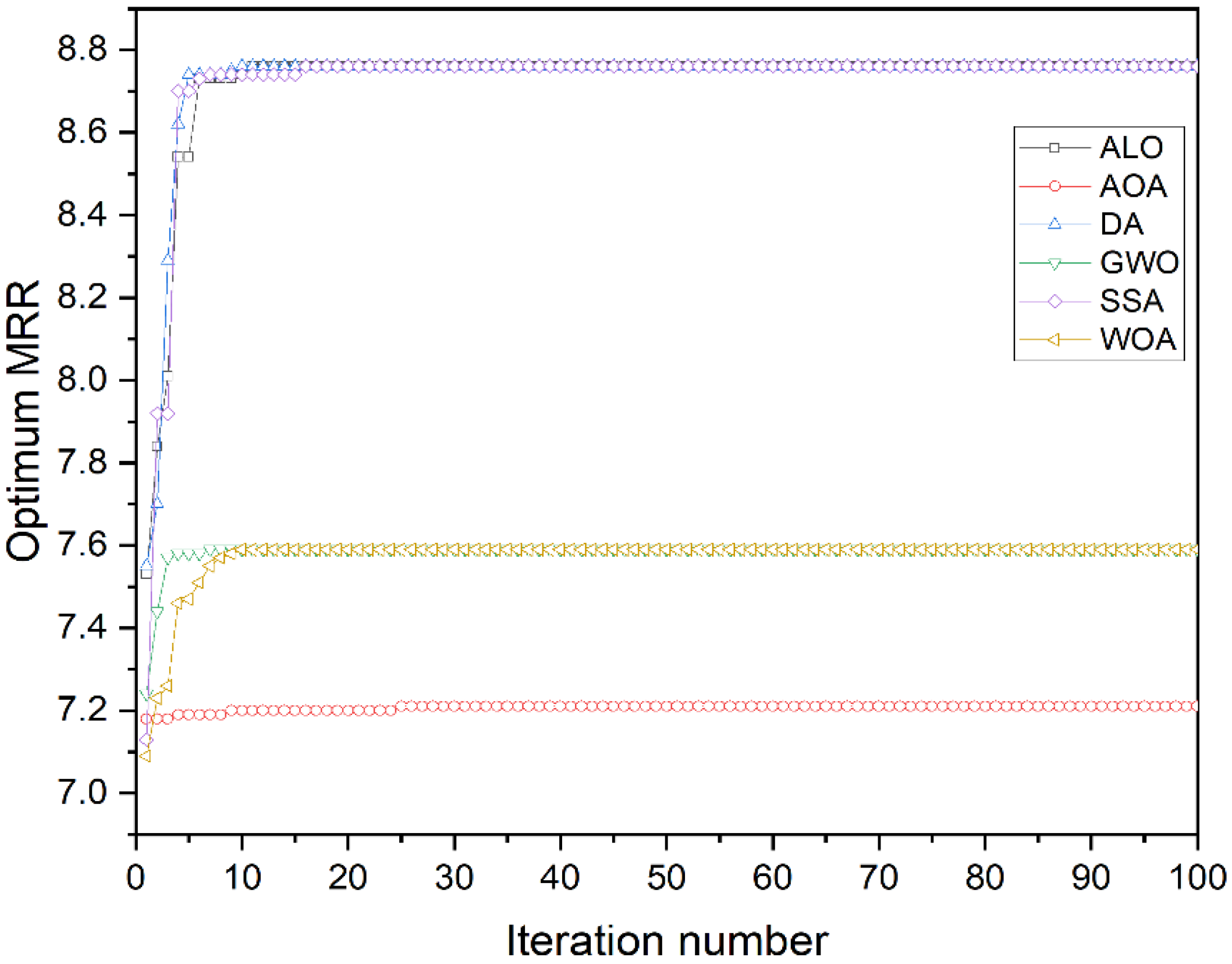
To make a fair comparison among all the selected algorithms, the number of search agents and iterations were limited to 30 and 100, respectively. Further, to eliminate any bias, each algorithm was independently run for 10 trials for each response. Figure 1 shows the convergence plot for the six metaheuristics for a typical trial while optimizing MRR.

It is observed from the plot that except for AOA, all the other algorithms had an appreciable increment in the best solution after the first few iterations. The convergence trend of GWO and WOA was seen to be similar for MRR optimization. ALO, DA and SSA showed monotonic improvement in the best solution search for the first few iterations, after which there was a negligible improvement in them.

Table 1. Statistical summary of 10 trials in optimizing MRR.

Algorithm	Mean	Standard Deviation	Median	Best	Worst	Success Rate
ALO	8.5306	0.4688	8.765	8.765	7.593	77%
AOA	7.9009	0.2689	7.962	8.188	7.21	0%
DA	8.765	0	8.765	8.765	8.765	100%
GWO	8.6478	0.3516	8.765	8.765	7.593	90%
SSA	8.765	0	8.765	8.765	8.765	100%
WOA	8.5697	0.4368	8.765	8.765	7.593	83%

shows the performance of the algorithms in terms of statistical parameters of 10 independent trials. It is observed that except for AOA, all other five algorithms reported the best value of 8.765. DA and SSA are observed to have a mean value of 8.765 for MRR optimization, indicating that these two algorithms were able to predict the best-known value in all 10 trials. Thus, the success rate (i.e., the ratio of the number of times the best-known value was achieved by the algorithm to the number of trials) for DA and SSA was 100%. The success rate for GWO, WOA and ALO and AOA was seen to be 90%, 83%, 77% and 0%, respectively.

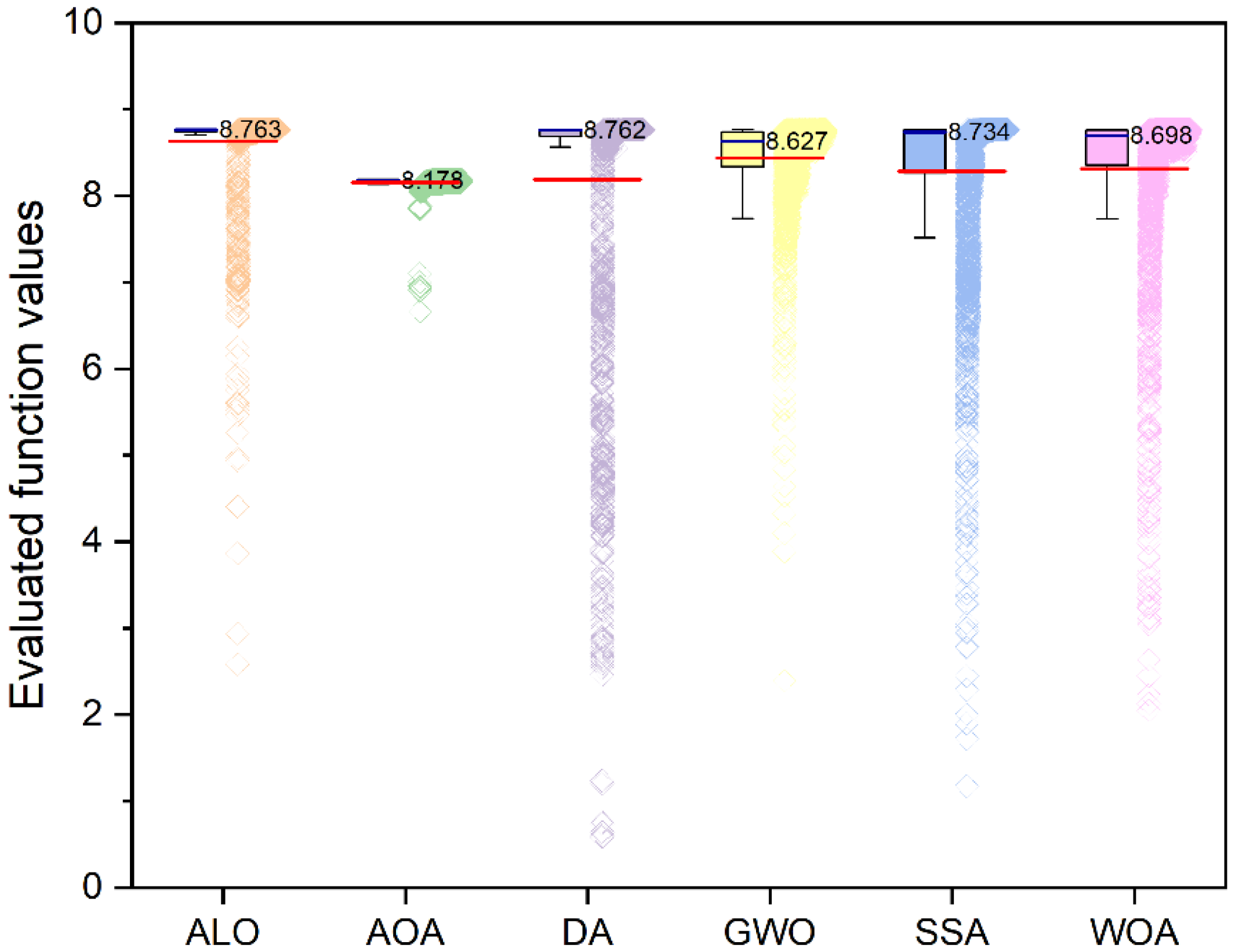
To delve deeper into the performance of the metaheuristics, the total function evaluations for each algorithm for a typical trial was plotted in the form of box plots in Figure 2.

In all of the other five algorithms, except AOA, the mean value of the total function evaluation was found to be significantly below the median line. This indicates that the lower 50th percentile of the total function evaluations had much smaller values as compared to the top 50th percentile. This could also be indicative of the fact that the algorithms initiated at a low function value and took a significant number of iterations to reach the high function value (optimal) zone. However, to draw a clear conclusion and avoid misinterpretation, it is important to look into this plot in conjunction with Table 1. For example, AOA’s mean and median values are very close to each other, with a very low spread of function evaluations. However, as seen from Table 1, it could not locate the best-known value. This would mean that despite the AOA randomly starting from a better initial position than the other algorithms, it was not able to improve its best-known solution iteratively. This is most likely due to AOA being tapped in the pit of local optima and its inability to navigate out of it. Among the other algorithms, GWO and ALO are seen to have a lower number of function evaluations with lower values, indicating that they had more rapid convergence towards the optimal zone.

The optimal process parameters and the MRR, as reported by the various metaheuristics, are presented in

Table 2. Comparison of current results with solutions from the literature for MRR optimization.

Algorithm	${\mathit{x}}_1$	${\mathit{x}}_2$	${\mathit{x}}_3$	${\mathit{x}}_4$	Optimum	% Improvement
Hewidy et al. [12]	6	0.5	7	0.5	6.57	-
ALO	3	0.3288	9	0.418	8.765	33.41%
AOA	3.16	0.4349	8.835	0.477	8.188	24.63%
DA	3	0.3288	9	0.417	8.765	33.41%
GWO	3	0.3288	9	0.417	8.765	33.41%
SSA	3	0.3288	9	0.417	8.765	33.41%
WOA	3	0.3288	9	0.417	8.765	33.41%

. With respect to the Hewidy et al. [12] solutions, AOA showed a 24.63% improvement. All the other algorithms reported a 33.41% improvement over the existing solutions in the literature.

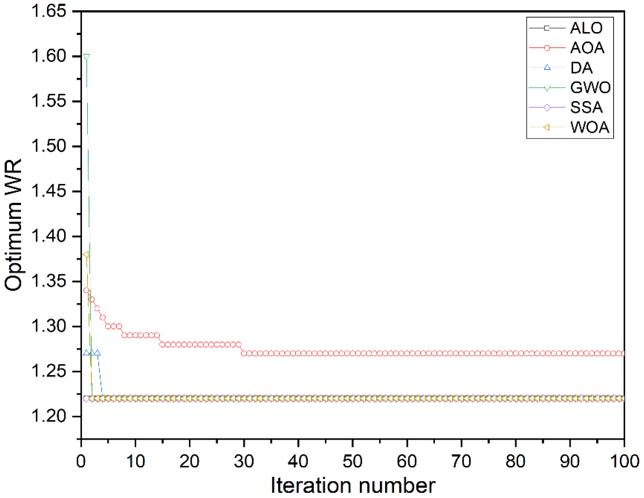
Figure 3 shows the convergence of the algorithms while optimizing the WR. It was observed that except for AOA, all other algorithms have a similar convergence trend.

Table 3. Statistical summary of 10 trials in optimizing WR.

Algorithm	Mean	Standard Deviation	Median	Best	Worst	Success Rate
ALO	1.216	0	1.216	1.216	1.216	100%
AOA	1.433	0.108	1.423	1.268	1.611	0%
DA	1.216	0	1.216	1.216	1.216	100%
GWO	1.216	0	1.216	1.216	1.216	100%
SSA	1.216	0	1.216	1.216	1.216	100%
WOA	1.216	0	1.216	1.216	1.216	100%

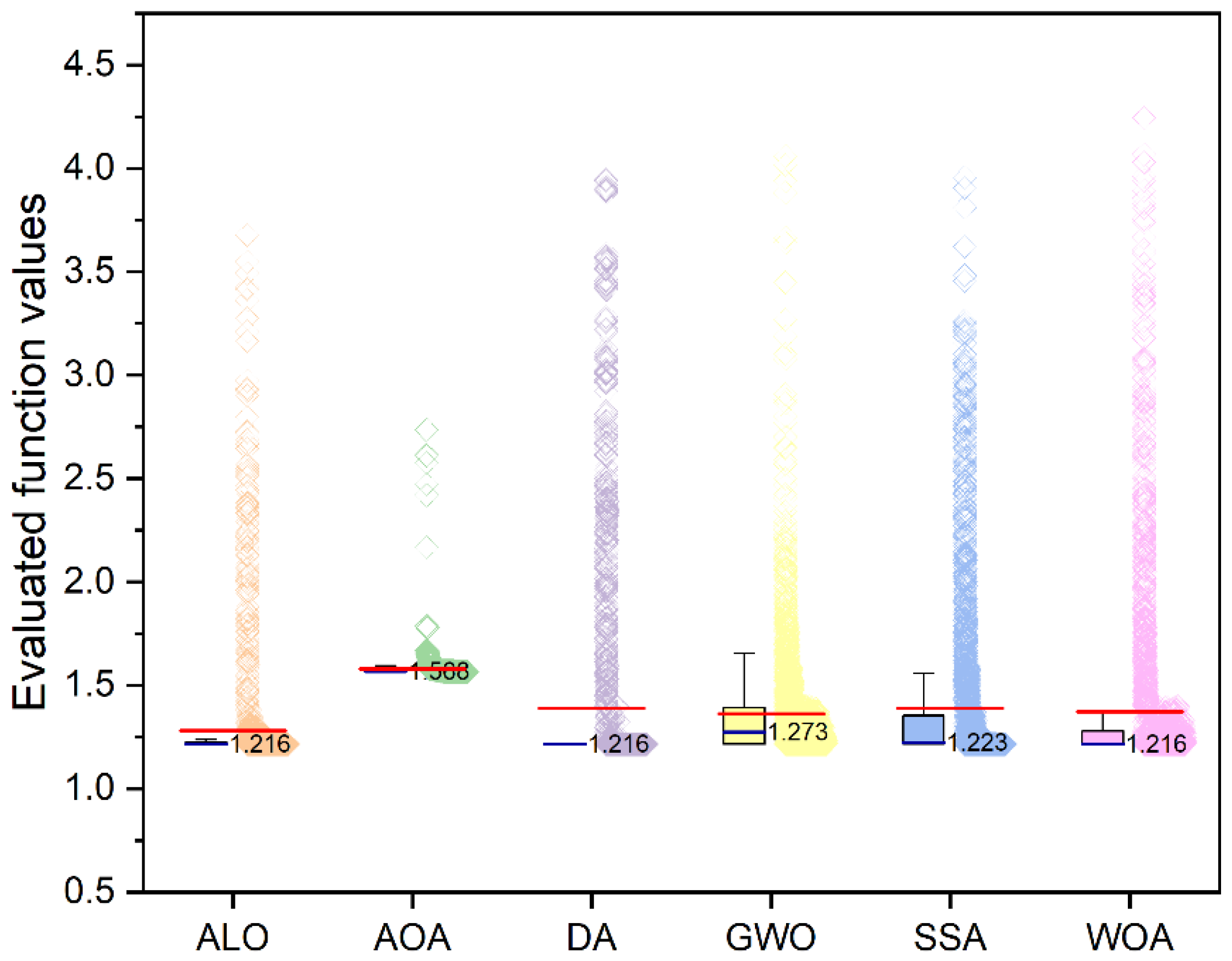
contains the statistical summary of the 10 independent trials of WR optimization. Like MRR optimization, in the case of WR, AOA was unable to locate the best-known optima. All the other five algorithms reported the best-known optima to be 1.216, an improvement of approximately 25% over the AOA results. As seen from Equation (42), the WR model was linear with only two process parameters. This may be the reason behind the 100% success rate reported by all the other five algorithms except AOA.

Figure 4 shows the spread of the total function evaluations during a typical trial while optimizing WR. The overall pattern of the spread and distribution of the function evaluations in Figure 4 is very similar to that in Figure 2. This indicates that the algorithms are unaffected by whether the optimization problem is a minimization or maximization type. GWO was seen to have the highest median function evaluation value among the algorithms. Moreover, the mean function evaluation value for GWO was very close to its median. This indicates that a very high percentage of GWO’s evaluated functions were in the optimal zone. This is generally preferred as it may be indicative of a high convergence rate.

The optimum process parameters for minimizing WR are presented in

Table 4. Comparison of current results with solutions from literature for WR optimization.

Algorithm	${\mathit{x}}_1$	${\mathit{x}}_4$	Optimum	% Improvement
Hewidy et al. [12]	7	0.7	4.24	-
ALO	3	0.3	1.216	71.32%
AOA	3	0.321	1.268	70.09%
DA	3	0.3	1.216	71.32%
GWO	3	0.3	1.216	71.32%
SSA	3	0.3	1.216	71.32%
WOA	3	0.3	1.216	71.32%

. With respect to Hewidy et al. [12], the current results are 70% better for AOA and 71.32% better for ALO, DA, GWO, SSA and WOA. Similarly, the optimum process parameters for minimizing SR are presented in

Table 5. Comparison of current results with solutions from the literature for SR optimization.

Algorithm	${\mathit{x}}_1$	${\mathit{x}}_2$	${\mathit{x}}_3$	${\mathit{x}}_4$	Optimum	% Improvement
Hewidy et al. [12]	5	0.75	9	0.5	2.2	-
ALO	4	0.623	8.2	0.62	1.151	47.68%
AOA	3.8	0.605	7.2	0.5	1.151	47.68%
DA	3.4	0.623	7.1	0.38	1.148	47.82%
GWO	4.6	0.678	7.3	0.54	1.148	47.82%
SSA	4.2	0.623	8.5	0.68	1.143	48.05%
WOA	5.2	0.568	9	0.6	1.143	48.05%

. In this case, the current ALO and AOA results are observed to be 47.68% better than Hewidy et al. [12]. On the other hand, DA and GWO results were 47.82% better, while SSA and WOA were 48.05% better than Hewidy et al. [12]. However, it is important to point out that all six algorithms reported varied in optimized values of the process parameters. This indicates that the objective function search space was, perhaps, multimodal. Therefore, it is worth mentioning that Hewidy et al. [12] used an RSM-based model to calculate the optimum values. The optimum values of responses obtained by Hewidy et al. [12] were MRR = 6.57 mm³/min, WR = 4.24 and SR = 2.20µm. The best-known optimum values obtained in this study were MRR = 8.765 mm³/min, WR = 1.216 and SR = 1.143 µm.

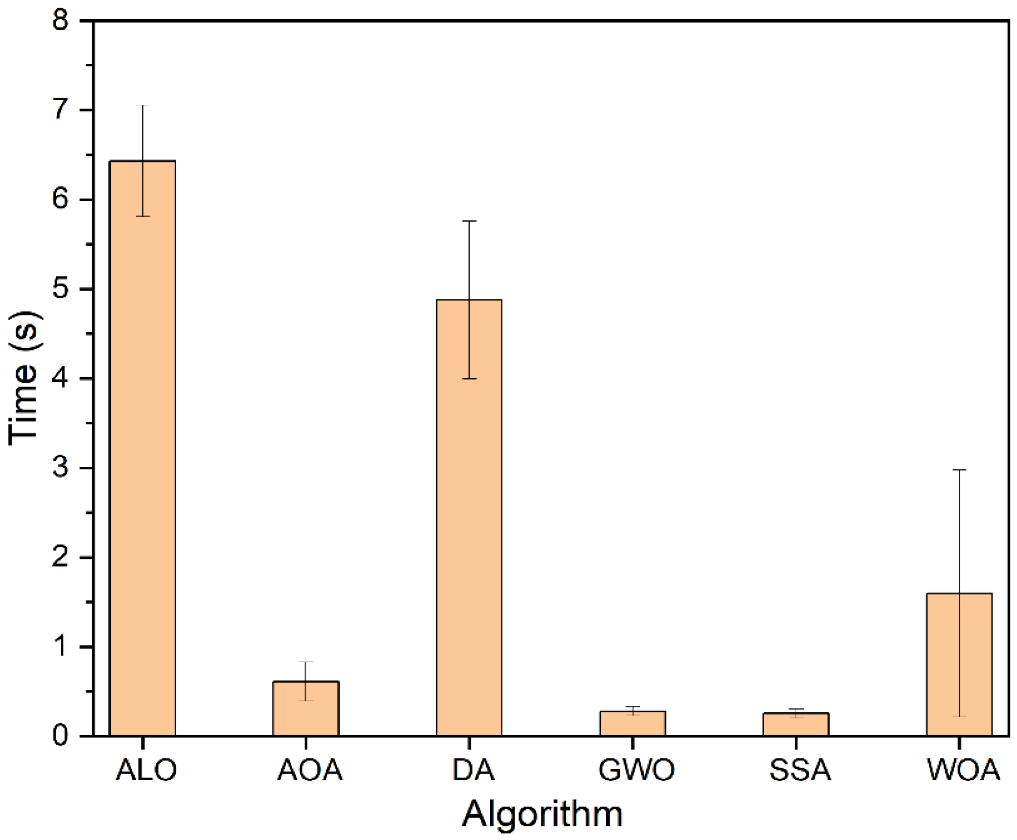
Though the same number of function evaluations (i.e., 30 × 100 = 3000) were carried out by each algorithm, some algorithms were expected to be faster than others. Thus, the CPU time of each algorithm was noted and averaged for 10 independent trials for each response. From Figure 5, it is observed that ALO, DA and WOA were the three most expensive algorithms, whereas SSA, GWO and AOA were the three least expensive. Nevertheless, the standard deviation of computational time for WOA was very high, indicating that in some instances, it may take a very short computation time. Perhaps this is because optimizing WR was very fast in optimizing the linear problem with only two variables.

All six recent algorithms performed better than the existing solutions by Hewidy et al. [12]. Hewidy et al. [12] used a desirability function-based approach, which is, in general, incapable of locating the global optima. The recent metaheuristics tested in this paper recorded at least 25%, 70% and 47% better solutions than Hewidy et al. [12] for MRR, WR and SR results. This improvement is perhaps due to the fact that the metaheuristics initiate a random population and algorithmically improve it over generations by continuously evolving the solutions. Based on the comprehensive evaluations of the algorithms on the three machining-related test functions, it can be summarized that despite AOA being the most recent algorithm among the six tested metaheuristics, it is not necessarily the best in locating the best-known optima. It is evident that the AOA is trapped in the local optima region, and for both the minimization type test functions, the solution of AOA was 1–2% poorer than the best-known optima. For the maximization-type test function, the best-known optima were observed to be roughly 9% better than the AOA’s solution. However, the computational time requirement of AOA was quite low, nearly on par with SSA and GWO. In terms of convergence, the SSA was observed to be the fastest. The median evaluated function value of SSA was seen to be quite a bit lower (for minimization problems) than its mean evaluated function value, indicating faster navigation to the optimal solution zone.

5. Conclusions

Machining process optimization is a necessary task for manufacturing industries and can lead to significant savings in material wastage, power consumption and tool wear and can improve productivity and efficiency of the process. Since a plethora of novel algorithms have been proposed in the recent past, with each having demonstrated capabilities in the literature, it is important to comprehensively compare them for their potential use in machining process optimization. In this article, six recently proposed nature-inspired algorithms, namely, ALO, AOA, DA, GWO, SSA and WOA, are comprehensively assessed, and the following conclusions were drawn.

• Based on the ability to navigate and find the optimal solution, the tested algorithms may be ranked as SSA > WOA > GWO > DA > ALO > AOA. Both SSA and WOA were able to locate the best solution for all three responses. However, SSA’s success rate was 100% as opposed to 83% of WOA.
• Based on the computational time, the tested algorithms may be ranked as SSA > GWO > AOA > WOA > DA > ALO. Both SSA and GWO had very minimal and similar computational requirements. However, SSA had a marginally lower standard deviation than GWO. As compared to ALO, SSA was observed to be about 25 times faster.
• The convergence of SSA was observed to be slightly better than its counterparts. GWO also showed fast convergence. AOA was prone to be trapped in local optima.
• As compared to the previous known best solutions, an average (on three responses) improvement of 50.8% and 47.47% was observed for ALO and AOA, respectively. DA and GWO showed a 50.85% improvement, whereas SSA and WOA recorded a 50.93% improvement.

The limitations of this study are that there are several advanced and hybrid variants of the algorithms, which were not considered in this paper. The study is also limited to one class of optimization problems. Nevertheless, the current optimization problems are of immense importance to industries. In the future, this study can be extended to incorporate an in-depth analysis of hybrid metaheuristics and the use of advanced quantum and chaotic enhancements to these algorithms. Optimization under uncertainty could also be an interesting area for their application.

References

1. Ramaswamy, A.; Perumal, A.V.; Jagadeesan, J.; Nagarajan, H.V. Optimization of WEDM process parameters for D3 die steel using RSM. Mater. Today Proc. 2021, 37, 2063–2069. [Google Scholar] [CrossRef]
2. Yong-Jie, M.; Wen-Xia, Y. Research progress of genetic algorithm. Appl. Res. Comput. 2012, 29, 1201–1206. [Google Scholar]
3. Zhou, C.; Gao, H.B.; Gao, L.; Zhang, W.G. Particle swarm optimization (PSO) algorithm. Appl. Res. Comput. 2003, 12, 7–11. [Google Scholar]
4. Gao, W.-F.; Liu, S.-Y. A modified artificial bee colony algorithm. Comput. Oper. Res. 2012, 39, 687–697. [Google Scholar] [CrossRef]
5. Faris, H.; Aljarah, I.; Al-Betar, M.A.; Mirjalili, S. Grey wolf optimizer: A review of recent variants and applications. Neural Comput. Appl. 2018, 30, 413–435. [Google Scholar] [CrossRef]
6. Abualigah, L.; Diabat, A.; Mirjalili, S.; Elaziz, M.A.; Gandomi, A.H. The arithmetic optimization algorithm. Comput. Methods Appl. Mech. Eng. 2021, 376, 113609. [Google Scholar] [CrossRef]
7. Abualigah, L.; Shehab, M.; Alshinwan, M.; Alabool, H. Salp swarm algorithm: A comprehensive survey. Neural Comput. Appl. 2020, 32, 11195–11215. [Google Scholar] [CrossRef]
8. Abualigah, L.; Shehab, M.; Alshinwan, M.; Mirjalili, S.; Elaziz, M.A. Ant Lion Optimizer: A Comprehensive Survey of Its Variants and Applications. Arch. Comput. Methods Eng. 2021, 28, 1397–1416. [Google Scholar] [CrossRef]
9. Gharehchopogh, F.S.; Gholizadeh, H. A comprehensive survey: Whale Optimization Algorithm and its applications. Swarm Evol. Comput. 2019, 48, 1–24. [Google Scholar] [CrossRef]
10. Gandomi, A.H.; Yang, X.-S.; Alavi, A.H.; Talatahari, S. Bat algorithm for constrained optimization tasks. Neural Comput. Appl. 2013, 22, 1239–1255. [Google Scholar] [CrossRef]
11. Meraihi, Y.; Ramdane-Cherif, A.; Acheli, D.; Mahseur, M. Dragonfly algorithm: A comprehensive review and applications. Neural Comput. Appl. 2020, 32, 16625–16646. [Google Scholar] [CrossRef]
12. Hewidy, M.S.; El-Taweel, T.A.; El-Safty, M.F. Modelling the machining parameters of wire electrical discharge machining of Inconel 601 using RSM. J. Mater. Processing Technol. 2005, 169, 328–336. [Google Scholar] [CrossRef]
13. Zhang, G.; Zhang, Z.; Guo, J.; Ming, W.; Li, M.; Huang, Y. Modeling and optimization of medium-speed WEDM process parameters for machining SKD11. Mater. Manuf. Processes 2013, 28, 1124–1132. [Google Scholar] [CrossRef]
14. Shihab, S.K. Optimization of WEDM process parameters for machining of friction-stir-welded 5754 aluminum alloy using Box–Behnken design of RSM. Arab. J. Sci. Eng. 2018, 43, 5017–5027. [Google Scholar] [CrossRef]
15. Chaudhary, A.; Sharma, S.; Verma, A. Optimization of WEDM process parameters for machining of heat treated ASSAB’88 tool steel using Response surface methodology (RSM). Mater. Today Proc. 2021. [Google Scholar] [CrossRef]
16. Mahapatra, S.S.; Patnaik, A. Optimization of wire electrical discharge machining (WEDM) process parameters using Taguchi method. Int. J. Adv. Manuf. Technol. 2007, 34, 911–925. [Google Scholar] [CrossRef]
17. Nayak, B.B.; Mahapatra, S.S. Optimization of WEDM process parameters using deep cryo-treated Inconel 718 as work material. Eng. Sci. Technol. Int. J. 2016, 19, 161–170. [Google Scholar] [CrossRef] [Green Version]
18. Mukherjee, R.; Chakraborty, S.; Samanta, S. Selection of wire electrical discharge machining process parameters using non-traditional optimization algorithms. Appl. Soft Comput. 2012, 12, 2506–2516. [Google Scholar] [CrossRef]
19. Mirjalili, S. The ant lion optimizer. Adv. Eng. Softw. 2015, 83, 80–98. [Google Scholar] [CrossRef]
20. Wang, J.; Du, P.; Niu, T.; Yang, W. A novel hybrid system based on a new proposed algorithm—Multi-Objective Whale Optimization Algorithm for wind speed forecasting. Appl. Energy 2017, 208, 344–360. [Google Scholar] [CrossRef]
21. Zawbaa, H.M.; Emary, E.; Grosan, C. Feature selection via chaotic antlion optimization. PLoS ONE 2016, 11, e0150652. [Google Scholar] [CrossRef] [Green Version]
22. Mafarja, M.; Eleyan, D.; Abdullah, S.; Mirjalili, S. S-shaped vs. V-shaped transfer functions for ant lion optimization algorithm in feature selection problem. In Proceedings of the International Conference on Future Networks and Distributed Systems, Cambridge, UK, 19 July 2017. [Google Scholar]
23. Mirjalili, S.; Jangir, P.; Saremi, S. Multi-objective ant lion optimizer: A multi-objective optimization algorithm for solving engineering problems. Appl. Intell. 2017, 46, 79–95. [Google Scholar] [CrossRef]
24. Mirjalili, S. Dragonfly algorithm: A new meta-heuristic optimization technique for solving single-objective, discrete, and multi-objective problems. Neural Comput. Appl. 2016, 27, 1053–1073. [Google Scholar] [CrossRef]
25. Mirjalili, S.; Mirjalili, S.M.; Lewis, A. Grey wolf optimizer. Adv. Eng. Softw. 2014, 69, 46–61. [Google Scholar] [CrossRef] [Green Version]
26. Mirjalili, S.; Gandomi, A.H.; Mirjalili, S.Z.; Saremi, S.; Faris, H.; Mirjalili, S.M. Salp Swarm Algorithm: A bio-inspired optimizer for engineering design problems. Adv. Eng. Softw. 2017, 114, 163–191. [Google Scholar] [CrossRef]
27. Mirjalili, S.; Lewis, A. The whale optimization algorithm. Adv. Eng. Softw. 2016, 95, 51–67. [Google Scholar] [CrossRef]
28. Hof, P.R.; van der Gucht, E. Structure of the cerebral cortex of the humpback whale, Megaptera novaeangliae (Cetacea, Mysticeti, Balaenopteridae). Anat. Rec. Adv. Integr. Anat. Evol. Biol. 2007, 290, 1–31. [Google Scholar] [CrossRef] [PubMed]
29. Hemeida, A.M.; Alkhalaf, S.; Mady, A.; Mahmoud, E.A.; Hussein, M.E.; Eldin, A.M.B. Implementation of nature-inspired optimization algorithms in some data mining tasks. Ain Shams Eng. J. 2020, 11, 309–318. [Google Scholar] [CrossRef]
30. Nasiri, J.; Khiyabani, F.M. A whale optimization algorithm (WOA) approach for clustering. Cogent Math. Stat. 2018, 5, 1483565. [Google Scholar] [CrossRef]
31. Oliva, D.; el Aziz, M.A.; Hassanien, A.E. Parameter estimation of photovoltaic cells using an improved chaotic whale optimization algorithm. Appl. Energy 2017, 200, 141–154. [Google Scholar] [CrossRef]
32. Watkins, W.A.; Schevill, W.E. Aerial observation of feeding behavior in four baleen whales: Eubalaena glacialis, Balaenoptera borealis, Megaptera novaeangliae, and Balaenoptera physalus. J. Mammal. 1979, 60, 155–163. [Google Scholar] [CrossRef]
33. Aljarah, I.; Faris, H.; Mirjalili, S. Optimizing connection weights in neural networks using the whale optimization algorithm. Soft Comput. 2018, 22, 1–15. [Google Scholar] [CrossRef]
Figure 1. Convergence of optimum MRR with respect to iterations.
Processes 10 00197 g001
Figure 2. Box plots denoting the spread of all function evaluations during MRR optimization in a typical independent run. The horizontal blue line (and numeric value) and the red line indicate the median and mean of all the function evaluations.
Processes 10 00197 g002
Figure 3. Convergence of optimum WR with respect to iterations.
Processes 10 00197 g003
Figure 4. Box plots denoting the spread of all the function evaluations during WR optimization in a typical independent run. The horizontal blue line (and numeric value) and the red line indicate the median and mean of all the function evaluations.
Processes 10 00197 g004
Figure 5. Average time taken by the algorithms in the optimization of the responses. The bars and whiskers denote the mean and standard deviation of 10 runs (3 responses X 10 independent runs/response).
Processes 10 00197 g005