Article

Numerical Modelling and Validation of Mixed-Mode Fracture Tests to Adhesive Joints Using J-Integral Concepts

by
Luís F. R. Neves
1,
Raul D. S. G. Campilho
1,2,*,
Isidro J. Sánchez-Arce
2,
Kouder Madani
3 and
Chander Prakash
4
1
Department of Mechanical Engineering, ISEP—School of Engineering, Polytechnic Institute of Porto, R. Dr. António Bernardino de Almeida, 431, 4200-072 Porto, Portugal
2
INEGI—Institute of Science and Innovation in Mechanical and Industrial Engineering—Pólo FEUP, Rua Dr. Roberto Frias, 400, 4200-465 Porto, Portugal
3
Department of Mechanical Engineering, University of Sidi Bel Abbes, BP 89 Cité Ben M’hidi, Sidi Bel Abbes 22000, Algeria
4
School of Mechanical Engineering, Lovely Professional University, Phagwara 144411, India
*
Author to whom correspondence should be addressed.
Processes 2022, 10(12), 2730; https://doi.org/10.3390/pr10122730
Submission received: 31 October 2022 / Revised: 6 December 2022 / Accepted: 15 December 2022 / Published: 17 December 2022
(This article belongs to the Special Issue Design of Adhesive Bonded Joints)

Abstract

:
The interest in the design and numerical modelling of adhesively-bonded components and structures for industrial application is increasing as a research topic. Although research on joint failure under pure mode is widespread, applied bonded joints are often subjected to a mixed mode loading at the crack tip, which is more complex than the pure mode and affects joint strength. Failure of these joints under loading is the objective of predictions through mathematical and numerical models, the latter based on the Finite Element Method (FEM), using Cohesive Zone Modelling (CZM). The Single leg bending (bending) testing is among those employed to study mixed mode loading. This work aims to validate the application of FEM-CZM to SLB joints. Thus, the geometries used for experimental testing were reproduced numerically and experimentally obtained properties were employed in these models. Upon the validation of the numerical technique, a parametric study involving the cohesive laws’ parameters is performed, identifying the parameters with the most influence on the joint behaviour. As a result, it was possible to numerically model SLB tests of adhesive joints and estimate the mixed-mode behaviour of different adhesives, which enables mixed-mode modelling and design of adhesive structures.

1. Introduction

Automotive, construction, aeronautical, and maritime industries extensively employ adhesive bonding for structural and cosmetic purposes. The design of such adhesive joints requires an a priori characterization of the materials involved. In addition, the joints themselves are also characterised, ensuring they fulfil the requirements they were designed for. In this regard, Budzik et al. [1] reviewed standard and non-standard tests for joints employed in several technological fields while Tserpes et al. [2] reviewed failure theories employed in the design of bonded structures. The mechanical properties of the adhesive are determined through experimental testing following the applicable standards, as described by da Silva et al. [3]. Moreover, in the adherends’ case, extensive testing is necessary for enhanced adherends, e.g., those studied in reference [4]. However, the behaviour of the adhesive within a joint also depends on geometric factors such as the adhesive layer’s thickness (tA) [5], material properties [6], and temperature [7]. In consequence, adhesive joints are characterised according to the expected loading conditions. Regarding the fracture behaviour of adhesive joints, there are three pure loading modes: traction (mode I), shear (mode II), and out-of-plane shear (mode III), as described by Dillard [8]. However, applications of adhesive joints often present a degree of mixing, i.e., more than one mode is present due to load solicitation. In this case, the failure occurs in mixed mode [8]. The critical energy release rate (GC) is among the Linear Elastic Fracture Mechanics (LEFM) methods employed to determine crack propagation, and it is necessary for computational simulations. Furthermore, GC has to be determined for each loading mode, i.e., mode I and mode II, through experimental tests. In the adhesive joints’ case, there are different experimental tests for this purpose, most of which are described by Pearson et al. [9] and Chaves et al. [10]. The tensile critical energy release rate (GIC) is often determined using the double-cantilever beam (DCB) test, while the shear critical energy release rate (GIIC) is determined using the end-notched flexure (ENF) test. On the other hand, Ji et al. [11] developed a mathematical model, based on the J-integral theory, to determine the tensile and shear energy release rates (GI and GII, respectively) under mixed-mode loading. Furthermore, the effect that tA has on the cohesive laws was evaluated. The proposed methodology consisted of experimental tests using the single-leg bending (SLB) test and followed by the mathematical approach to obtain the cohesive laws. It was found that tA has a proportional effect on GI, GII, and joint strength. However, it does not affect the normalised tension used for the cohesive laws.
Cases of experimental characterisation of adhesives using the DCB and ENF tests are often found in the literature. For example, Faneco et al. [12] employed both DCB and ENF tests to characterise a polyurethane structural adhesive, the SikaForce® 7752, for industrial use. The specimens tested for both cases were composed of aluminium adherends, and tA = 1 mm. Six specimens of each case were tested. Upon completing the experimental campaign, good repeatability of the results was observed, indicating good control in the specimen preparation and testing. Subsequently, GIC and GIIC were obtained using three different methods. This approach was also followed by Cardoso et al. [13] to characterise another polyurethane structural adhesive, the SikaPower® 1277, also for industrial use. The specimen dimensions and tA were similar to those used by Faneco et al. [12]. In addition, the results also showed good repeatability, confirming that good control was had on specimen preparation and experimental procedure. Regarding the experimental procedures, both DCB and ENF were described by da Silva et al. [3] and Pearson et al. [9]. Similarly, there are experimental tests aimed at mixed-mode loading such as the cracked-lap shear (CLS) [14], mixed-mode bending (MMB) [15], and the SLB [16]. Testing between the SLB and ENF configurations is similar, hence no extra laboratory equipment is necessary, making this test convenient [9]. Furthermore, the results obtained from the mixed-mode tests together with those from pure mode allow for determining the fracture envelopes, which show how the joint behaves under different loading conditions [9] and are useful for design purposes. The SLB test has been used to determine fracture envelopes of different adhesives. For example, Santos and Campilho [17] studied the fracture behaviour of three different adhesives, from brittle to ductile, using this test. The joints had composite adherends and tA = 1 mm. The results from the experimental testing were repeatable and consistent. Subsequently, the values of GI and GII were obtained using six different reduction methods and, again, good repeatability was observed regardless of the method. Then, these results together with the results from GIC and GIIC lead to obtaining the fracture envelopes and the exponent values for the power laws. More recently, Loureiro et al. [18] performed a similar experimental campaign testing seven specimens per adhesive type, for a total of three adhesive types. In this case, the J-integral method was used to calculate GI and GII. The results showed low variability regardless of the adhesive type. Then, the fracture envelopes were obtained, and the exponents of the power laws were calculated. These results agreed with previous research, indicating their validity. Furthermore, the parameters obtained in these works are necessary for the numerical modelling of bonded joints [17,18].
Numerical modelling using the Finite Element Method (FEM) has been employed to study adhesive joints for a long time, and Adams and Peppiatt [19] are among the pioneers in this regard. More recently, cohesive zone modelling (CZM) was included in FEM, allowing one to predict joint strength, and even debonding, with good accuracy [2]. However, the cohesive laws must be properly chosen, from which the bi-linear or triangular law is a good compromise between accuracy and computational cost [20]. The parameters necessary to model the cohesive behaviour of the adhesive layer are obtained from the experimental tests listed above. Reis et al. [21] experimentally tested SLB specimens made of solid composite material (carbon fibre and polyamide), and then, numerically reproduced the experimental setup with the aim of assessing the suitability of this composite as an alternative to thermoset ones. The joints were modelled as two-dimensional (2D) plane-strain cases using FEM and CZM, trapezoidal cohesive laws were employed, and the numerical results were similar to the experimental data. Then, it was found that the chosen composite was a suitable alternative to conventional thermoset composites. Similarly, SLB for adhesive joints were modelled by Santos and Campilho [17] and Loureiro et al. [18]. In both cases, the numerical models reproduced the experimental setup performed by the authors. The numerical models were also 2D assuming plane-strain conditions and triangular cohesive laws were used. In these two cases, three different adhesive types were evaluated. Regardless of the adhesive type, the numerical results agreed with the experimental data gathered a priori, validating the numerical methodologies. Although the described research reached a good agreement between numerical and experimental data, no parametric studies of the cohesive parameters were reported. In this regard, Alfano [20] suggested that these sensitivity analyses are worth exploring. Furthermore, contrary to other joint configurations, the SLB has little presence in the literature, even though it provides data for mixed-mode fracture.
This work aims to validate the application of FEM-CZM to the analysis of SLB adhesive joints. Thus, the geometries used for experimental testing were reproduced numerically, and experimentally obtained properties were employed in these models. Upon the validation of the numerical technique, a parametric study involving the cohesive laws’ parameters is performed, aiming to evaluate their influence on the overall behaviour of this type of adhesive joint.

2. Materials and Methods
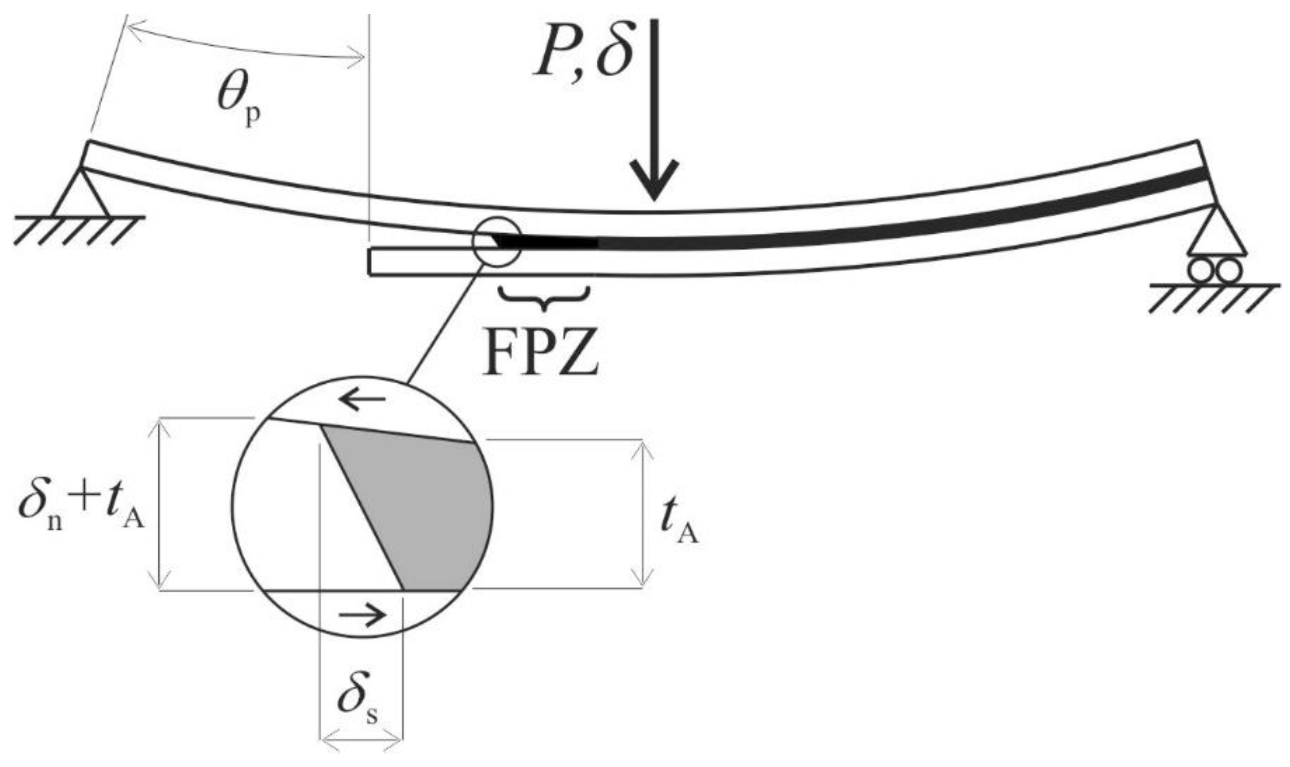
2.1. Geometry

The SLB specimen has two adherends bonded together, one of them shorter and placed below, to induce mixed-mode loading during bending, i.e., three-point bending. The initial crack (a0) should obey a relationship of 70% with respect to the half-span between supports (L), i.e., a0 = 0.7L. A schematic of this specimen’s geometry is shown in Figure 1 (P is the load and δ is the displacement). The SLB geometry is based on the work of Yoon and Hong [22], later expanded by Chaves et al. [10].
In this work, 2L = 250 mm, the adherend thickness (h) = 3 mm, tA = 1 mm, out-of-plane-width (B) = 15 mm, and a0 ≈ 87.5 mm. The overall lengths of the upper and lower adherends were 280 mm and 200 mm, respectively.

2.2. Materials

For this work, three adhesive types were considered, namely the Araldite® AV138, Araldite® 2015, and SikaForce® 7752, varying from brittle to ductile. The Araldite® adhesives are epoxy-based while the SikaForce® is polyurethane-based. These adhesives were experimentally characterised in previous works [12,23,24], and their mechanical properties are listed in Table 1. In addition, the mechanical properties that were obtained employed the appropriate standards, while the fracture properties were obtained from bonded CFRP specimens. The experimental procedures for these tests were described in detail by da Silva et al. [25].
The adherends were cut from carbon-fibre reinforced plastic (CFRP) plates with a thickness of 3 mm. These plates were manufactured in-house using 20 layers of carbon-epoxy pre-preg (SEAL Texipreg HS 160 RM, Legnano, Italy) with an individual thickness of 0.15 mm. The layers were manually laid-up unidirectionally, i.e., [0]20. Then, the plates were pressed at 2 bar and 130 °C for one hour using a dedicated press with hot plates (200 kN press by Gislotica Lda; Perafita, Porto, Portugal). The manufacturing procedure for the composite plates is described in better detail by Santos and Campilho [17]. Regarding the mechanical properties of the prepreg used, these are listed in Table 2.

2.3. Experimental Details

In this work, three different adhesives were evaluated, and seven specimens per adhesive type were prepared. Therefore, the adherends were cut from the composite plates, mentioned in the previous section, to the appropriate sizes (Figure 1). The cutting of the specimens was done using an abrasive saw with a diamond wheel suitable for composite materials. In addition, several shims were cut and prepared to ensure the desired tA. Once cut, the adherends and shims were prepared for the bonding process by following the procedure described by Faneco et al. [12]. Furthermore, a razor blade was placed at the end of the bond line, leading to the initial crack notch. Then, the adherends were laid on a flat surface, the spacers were placed, the respective adhesive was applied, and the second adherend was placed on top and aligned. The adherends were kept aligned during the curing time using spring-loaded clamps located in the areas where the shims are, hence ensuring the desired tA. All the specimens were left to cure at room temperature for three days in the case of both Araldite® adhesives, and five days for the SikaForce®. After the curing process, the shims were removed, and all the excess of adhesive was carefully trimmed using mechanical means. Subsequently, each specimen was marked by adhesive type and specimen number, and the actual dimensions of each one were documented. In order to ease the visualisation and measurement of the crack propagation, one of the side faces of the specimen, including the adhesive layer, was painted in white and a scale was attached to the adherend, as shown in Figure 2. Then, the individual values of a0 were registered. These processes are described in more detail by da Silva et al. [3].
Once all the specimens were prepared and measured, each one was tested using a universal testing machine or UTM (Shimadzu AG-X-100) with a 100 kN load cell. The bending loading was imposed through a fixture compatible with the UTM, as shown in Figure 3.
The testing speeds employed were 0.35 mm/min, 0.8 mm/min, and 3 mm/min for the Araldite® AV138, Araldite® 2015, and SikaForce® 7752, respectively. Furthermore, the crack length (a) was measured using high-resolution pictures focused on the scale attached to the specimen (Figure 2). The pictures were taken every 5 s, with the first photograph taken at the beginning of the test. Therefore, the pictures are related to the UTM data using the time stamps. The experimental setup is depicted in Figure 3. Finally, the tests were run until a reached the loading point (Figure 1).

2.4. J-Integral Formulation

The J-integral formulation was used to estimate the fracture energies from the SLB tests. This contour integral was proposed by Rice [28] in the 1960’s to calculate the strain concentration near cracks and notches. Currently, this technique has been extended to several fracture tests, such as the DCB (mode I), ENF (mode II), and SLB (mixed mode). The formulae following in this work were proposed by Ji et al. [11] within the scope of adhesive layer characterisation, ultimately leading to closed-form expressions of GI and GII, enabling one to obtain the energies and mode-partitioned CZM laws by a differentiation procedure. To make this procedure possible, three relevant geometric variables, apart from the typical P and δ, should be measured during the test (Figure 4): the relative rotation between the two adherends at the loading line (θP), the normal separation at the crack tip (δn), and the shear separation at the crack tip (δs). GI is given by:
G I δ n = 0 δ n t n δ n d δ n = P 4 θ P
In this expression, tn is the current tensile stress. On the other hand, GII can be calculated as:
G II δ s = 0 δ s t s δ s d δ s = 1 2 h D 2 Q T 2 a 2 + h Q T 2 D δ 0 2 A + h 2 2 D
where ts represents the current shear stress, D is the beam bending stiffness (assuming identical adherends), A is the beam axial stiffness, and QT is the resultant of shear forces acting on the bonded SLB specimen. After having GI and GII as a function of δn and δs, respectively, the direct CZM law estimation method gives the tensile (tn-δn) and shear cohesive laws (ts-δs), by differentiating the GI-δn and GII-δs curves, respectively, resulting from the former expressions:
t n δ n = d G I δ n d δ n = d P 4 θ P d δ n
and
t s δ s = d G II δ s d δ s = d 1 2 h D 2 Q T 2 a 2 + h Q T 2 D δ s 2 A + h 2 2 D d δ s
As previously mentioned, θp, δn, and δs require continuous measurement during the SLB tests. Data acquisition can rely on mechanical sensors such as linear variable differential transformers (LVDT) or optical methods, including digital image correlation (DIC). The procedure in this work involved using an optical method founded on taking high-resolution pictures during the tests (Figure 3), and then performing a vector and geometric analysis of the images captured during the tests by imaging software to produce a value of θp, δn, and δs for each picture, which can be correlated with the testing machine data. More details about this procedure and geometrical extraction of the parameters from the pictures can be found in previous work [18].
The methodology just described allows one to obtain the current values of GI and GII, so they can be correlated within a plot, known as the fracture envelope [9]. Then, the mode-mixity is defined through a power law [29], as follows:
G I G IC α + G II G IIC β = 1 ,
where the critical values of GIC and GIIC are known from the characterisation of the material, i.e., as reported in Table 1. The exponents α and β define the shape of the envelope, being commonly considered equal [30], so α = β, with common values of 0.5, 1, 1.5, and 2. Then, the power law (Equation (5)) is plotted for each value of α. Finally, comparing the points where the current GI and GII lay in relation to the envelopes provides the exponent α for the analysed test.

2.5. Numerical Modelling

CZM modelling of the SLB specimens in Abaqus® is employed in this work to validate the CZM laws and fracture envelopes defined in the experimental part. The simulation is geometrically non-linear, which is mandatory for the magnitude of involved deformations. The mesh refinement was optimised, with higher refinement at the crack growth region and contact with the loading cylinders (as shown in Figure 5, together with the boundary conditions). Since the models are 2D, the adherends were discretised by plane-strain four-node solid finite elements (CPE4 from Abaqus®), and the adhesive by four-node cohesive elements (COH2D4 from Abaqus®). Bias effects were used to reduce the computational effort while concentrating elements where needed: six elements were considered through-thickness in the adherends with a minimum size of 0.1 mm and a maximum size of 0.2 mm, showing higher refinement at the free faces [31]. The element size in the bond line was 0.5 mm × 1 mm from the crack notch until the centre support (L from Figure 1) while the remaining size was 1 mm × 1 mm. The mesh size in the vicinities of the rollers was finer to reduce element distortion. In this case, the element size was 0.05 mm. The element size on regions of low interest was 1 mm. The models were composed of 6144 CPE4 elements, 400 COH2D4 elements, and a total of 8676 nodes. It is worth noting that the mesh sizes were chosen from the authors’ previous experience with similar finite element models. Furthermore, the chosen mesh size is also in agreement with those reported in the literature for similar cases. Thus, mesh sensitivity analyses were not required.
Following the geometry shown in Figure 1, the substrates are supported and loaded through rollers. Therefore, the centres of the supporting rollers were fixed in both directions (UX = UY = 0), which reproduces the experimental setup. In addition, the upper roller applying the displacement was constrained in the horizontal direction (UX = 0) while its vertical displacement corresponds to the displacement imposed by the UTM, i.e., UY = δ. Furthermore, the point of contact of the upper roller was also constrained in the horizontal direction, as shown in Figure 5, reducing the degrees of freedom of the system. Nevertheless, no horizontal displacement was observed during the experimental testing. The interactions between rollers and substrates were defined through surface-to-surface frictionless contact conditions with hard behaviour in the normal direction.
The modelling procedure consisted of setting one individual model for each experimental test, including the measured dimensions and a0, for maximum accuracy. The adhesive layer was modelled by one row of four-node cohesive elements whose definition is based on the pure tensile and shear CZM laws; in this case, triangular cohesive laws were employed, of which, the relevant properties (E, G, and tensile cohesive strength or tn0, shear cohesive strength or ts0, GIC, and GIIC) were taken from Table 1. To numerically establish the mixed-mode behaviour, it is necessary to know the power-law exponent, which is calculated from the experimental data, namely when building the fracture envelopes for each adhesive. Thus, this exponent may differ between tested adhesives. The comparison between the experimental data and numerical predictions in the results section will be able to validate the CZM law and respective mixed-mode criteria for strength prediction of bonded joints.

2.6. Triangular CZM

CZM modelling relies on the establishment of stress-relative displacement laws or CZM laws that link paired nodes of the cohesive elements. The CZM laws reproduce the materials’ elastic behaviour up to reaching the cohesive strength in the respective loading mode and the damage or softening process that follows, to simulate the material degradation until failure and respective crack growth. GIC and GIIC correspond to the area beneath the tensile and shear CZM laws, respectively. When considering pure mode, damage grows at a set of paired nodes when stresses are cancelled at the end of softening. On the other hand, under mixed mode damage growth is ruled by energetic criteria that combine the individual loading modes [32]. Triangular CZM laws were considered in this work, i.e., with linear softening, for pure and mixed-mode analysis. A schematic representation of this law is shown in Figure 6. In the pure mode laws, the linear part of the curve up to the cohesive strength is defined by a matrix that relates stresses with strains, and with E and ν as main parameters. Although damage initiation under mixed mode can be assessed by different criteria, this work uses the quadratic nominal stress criterion. Upon reaching the mixed-mode cohesive strength (tm0), the material stiffness is degraded. Damage growth, i.e., separation of the paired nodes, is predicted using a power law expression based on the current GI and GII (Equation (5)), initially proposed by Wu and Reuter [29]. In this work, it was considered that α = β, whose numerical value was estimated using experimental data (Section 2.5) and subsequently validated numerically. Further details of this model are given in reference [23].

3. Results and Discussions
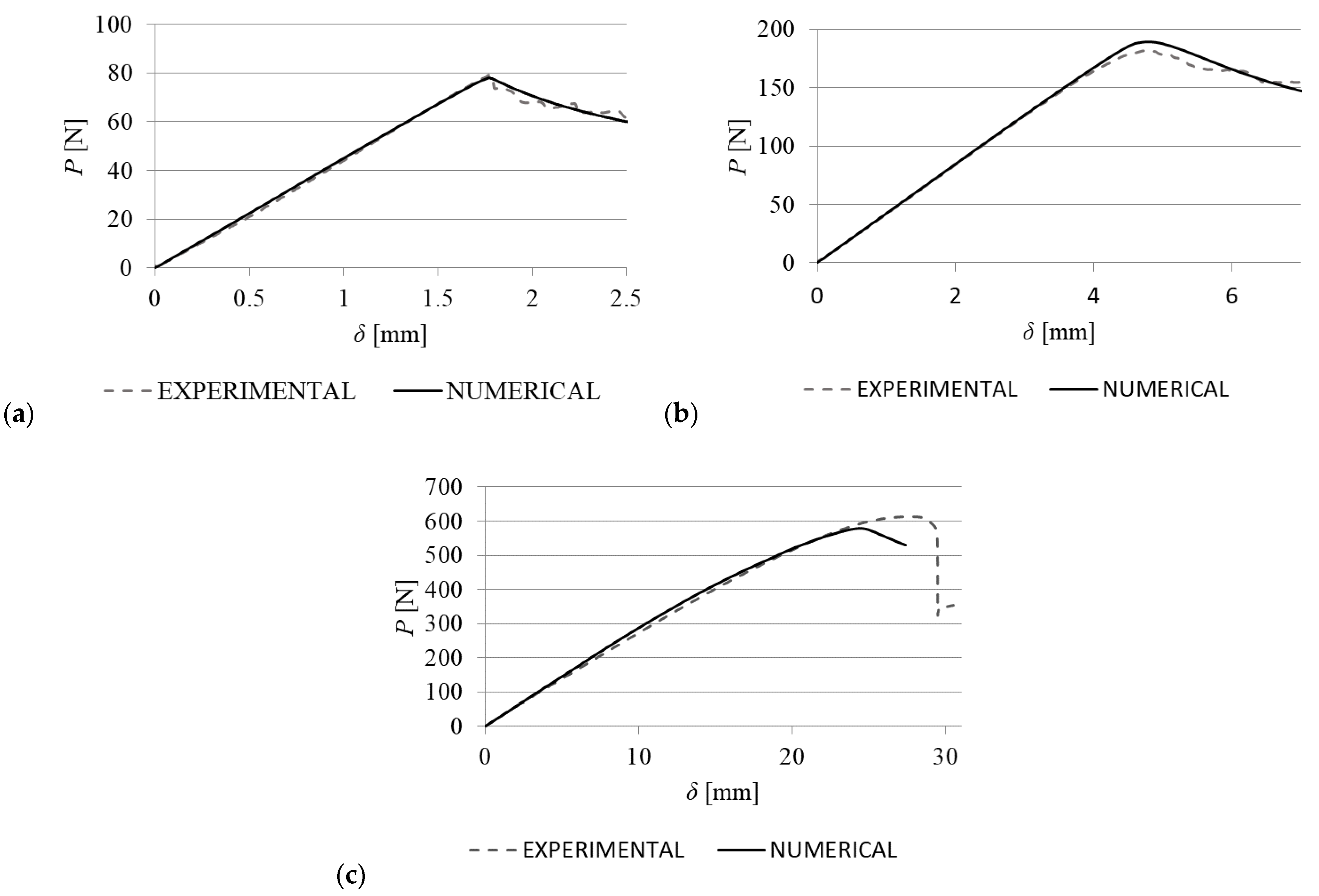
3.1. P-δ Curves

The P-δ curves were the initially collected data for the tests, leading to the subsequent fracture analyses. Figure 7a gives an example of the correlation between specimens of the same adhesive (Araldite® 2015), and Figure 7b shows sample P-δ curves for each of the three adhesives, to visually reinforce the differences between adhesives. Figure 7a emphasises the repeatability of the test data, showing that the specimens were fabricated and tested under identical conditions. This agreement is also valid for the other two adhesives tested in this work. Minor elastic stiffness variations take place because of differences in a0 between specimens. Figure 7b shows a markedly different efficiency of the adhesives, which relates to mixed-mode fracture, made visible by the different maximum load (Pm) and maximum load displacement (δPm). In the Araldite® AV138, the evolution of P with δ is predominantly linear until the crack begins to propagate. After crack onset, few specimens showed unstable crack propagation, which is considered to be related to the presence of small defects in a brittle adhesive, triggering catastrophic failure [33]. For this adhesive, Pm = 81.1 ± 4.5 N and δPm = 2.11 ± 0.23 mm. The Araldite® 2015 shows an improved fracture behaviour, due to much higher Pm and δPm (Pm = 204.2 ± 12.8 N and δPm = 5.6 ± 5.58 mm). Although this adhesive possesses lower stiffness and tensile strength than the Araldite® AV138, it also has higher ductility, hence performs better within the scope of fracture tests. Moreover, the sample P-δ curve reveals non-negligible softening up to Pm, associated to the creation of a bigger FPZ that develops at the crack tip before crack onset. Finally, the SikaForce® 7752 presents the best toughness results, with Pm = 630.3 ± 26.0 N and δPm = 28.4 ± 1.22 mm. Compared to the previous adhesives, there is a marked softening before Pm, denoting the large dimensions’ FPZ taking place before crack growth, accompanied by a softer transition to failure. These differences should reflect in the fracture measurements that follow.

3.2. Toughness Estimation

Estimation of GI and GII for all specimens was performed as specified in Section 2.4, beginning with plotting θp, δn, and δs vs. δ curves up to crack initiation, for application of the J-integral formulation. To make the curves smoother, all curves were subjected to polynomial fitting, which was successful in the sense that it was possible to replicate the experimental evolution with accuracy. It was found that the evolution of δn and δs with δ is exponential [34], while the θP–δ curves are nearly linear. After applying the formulae of Section 2.4, namely expressions (1) and (2), it was possible to derive the GIδn and GIIδs plots up to crack initiation, which are on the basis of the CZM law calculation by expressions (3) and (4). Figure 8a shows sample curves for an SLB specimen bonded with the Araldite® 2015. Normally, these curves are divided into three portions: the first part with a slow increase of GI or GII, followed by a marked increase, whose maximum slope gives tn0 or ts0, and finally, the attainment of a steady-state value of GI or GII, corresponding to crack initiation. This behaviour was generally observed in the tested specimens, although with a few inconsistencies in some specimens due to experimental issues and fitting difficulties. The main problem was the curve initiation with a non-nil slope, which then reflected on non-nil stress at the initiation of the respective CZM laws. The correlation of this data with a, measured from the experimental tests, gives the R-curves, of which an example is presented in Figure 8b for the SLB bonded with the Araldite® 2015. For all adhesives, it was found that the tensile and shear plots are identical, although with GI > GII. All R-curves begin at the a value of a0, corresponding to the steep increase of GI or GII triggering crack initiation, followed by a theoretically horizontal evolution of GI or GII, in which the critical values are measured by averaging. The average and standard deviation data for each adhesive (including GI and GII) are given in Table 3. The maximum coefficient of variation occurred for GII of the Araldite® 2015, of 6.1%. On the other hand, the difference was high between adhesives, reflecting their known brittleness or ductility.

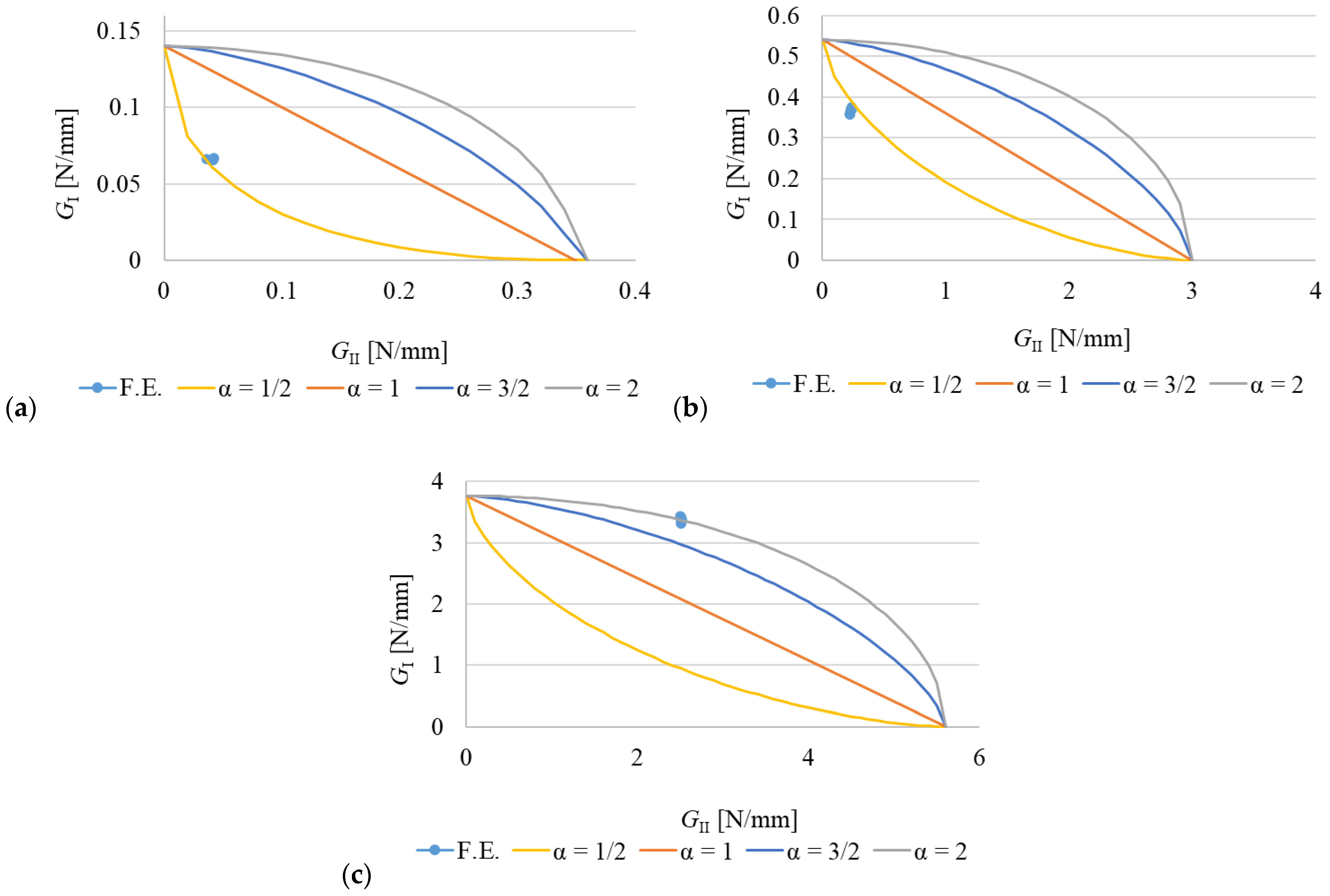
3.3. Fracture Envelope

The fracture envelopes enable framing the mixed-mode behaviour of the adhesives by plotting the GI/GII data points against idealised power law criteria having as limits the GIC and GIIC of pure tensile (DCB) and shear (ENF) results [17]. The power law expressions are obtained from Equation (5), considering α = β. Thus, from this point on, the exponent in the power law expression is cited as α. Different power laws (α = 1/2, 1, 3/2, and 2) are evaluated to reproduce the experimental mixed-mode behaviour of each tested adhesive. Figure 9 presents the experimental fracture envelopes for the three adhesives separately.
Figure 9a, relating to the Araldite® AV138, reveals proximal data points, leading to coefficients of variation of approximately 4% for both GI and GII. For this adhesive, α = 1/2 reveals to be an accurate representation since all data points are close to this criterion. Figure 9b presents the fracture envelope for the Araldite® 2015, and highlights the good agreement between specimens, materialised by coefficients of variation of approximately 2% (GI) and 6% (GII). Although in this case α = 1/2 is identically the best option for mixed-mode failure prediction, the data points are clearly above the criterion. Figure 9c, representing the SikaForce® 7752 fracture envelope, depicts coefficients of variation below 2% for both loading modes but reveals a markedly different behaviour to the other two adhesives. For this adhesive, the data points are situated near the α = 2 criterion, which may be related to the polyurethane base and associated ductility.

3.4. CZM Laws

The CZM laws in both modes of loading were estimated by the direct method, as described in Section 2.4. To apply expressions (3) and (4), applicable to the mode I and II laws, respectively, it was previously necessary to approximate the data points of the GI-δn and GII-δs functions by polynomial functions, individually for each specimen, for further differentiation. Figure 10 represents, as an example, the full set of tensile (a) and shear (b) CZM laws for the Araldite® 2015, which also represents the degree of correspondence for the other two adhesives. The agreement was generally very good regarding the sets of tensile or shear CZM laws of a given adhesive, including the elastic portion up to tn0 or ts0, the values of tn0 and ts0, and also the tensile and shear failure displacements (δnf and δsf, respectively). Typically, the tn-δn and ts-δs laws do not initiate with nil stresses, as expected, due to using polynomial approximations. The Araldite® AV138 CZM laws revealed a triangular-like form under tensile and shear assumptions. The collected data for this adhesive was as follows: tn0 ≈ 35 MPa, ts0 ≈ 18 MPa, δnf ≈ 0.01 mm, and δsf ≈ 0.02 mm. The values of δnf and δsf are much reduced, which can be associated with brittleness and stiff behaviour. The CZM laws of the Araldite® 2015, corresponding to the sample curves shown in Figure 10, equally depict a triangular-like shape, but ductility signs were visible near failure. The collected information for this adhesive was as follows: tn0 ≈ 17 MPa, ts0 ≈ 7 MPa, δnf ≈ 0.05 mm, and δsf ≈ 0.1 mm. Comparison of these values with those of the Araldite® AV138 gives an increase of δnf of 421%, and δsf of 358%. The SikaForce® 7752 CZM laws showed a significantly different shape compared to the former two adhesives, namely in the shear CZM law, which revealed a large steady-state region with significant stresses, i.e., resembling a trapezoidal shape CZM. This result arises from the large ductility of the SikaForce® 7752, and it is considered that this adhesive could be better modelled by a trapezoidal law [20]. The average data for the SikaForce® 7752 led to the smallest tn0 and ts0, and the biggest δnf and δsf (tn0 ≈ 6 MPa, ts0 ≈ 5 MPa, δnf ≈ 1.6 mm, and δsf ≈ 1 mm). The δnf and δsf values are much higher than for the other adhesives, with more significance for δnf. Considering all adhesives and both loading modes, the coefficients of variations were typically under 10% for tn0 and ts0, while δnf and δsf could not comply with this standard and showed higher variations.

3.5. CZM Law Validation

Validation of the cohesive laws was done through the comparison between experimental and numerical values of Pm and δPm. Regarding the values of GIC and GIIC, i.e., pure mode, data from the literature were used due to the mode-mixity found in the SLB. Then, the experimentally defined α for each adhesive was assigned to each case tested. Starting with the data of the Araldite® AV138, the numerical Pm was close to the experimental one, being on average 2.6% lower (range 0.3% to −6.0%). Similarly, the numerical δ was 2.2% lower than the experimental values (range 1.4% to −7.9%). The highest difference in both values was observed on Specimen #1. Despite this fact, a good agreement between numerical and experimental data was attained. As an example, the comparison for Specimen #3 is shown in Figure 11a. Following, in the Araldite® 2015 a similar trend was observed, and the numerical Pm was on average 3.3% lower than the experimental value (range 3.8% to −7.2%). The numerical δ was on average 5.9% lower than its experimental counterpart (range 0% to −11.0%). The overall shapes of the numerical and experimental curves also matched. For example, the comparison for Specimen #3 is shown in Figure 11b. For the SikaForce® 7752, the numerical Pm was on average 7.0% lower than the experimental values (range −1.7% to −12.5%). In this case, the numerical models underpredicted δ on average by −14.0% (range −9.1% to −19.26%). Regardless of these differences, the P-δ curves, both numerical and experimental, showed similar behaviours. For example, the comparison corresponding to Specimen #3 is shown in Figure 11c.
Subsequently, the values of GIC were determined from all the experimental and numerical cases and then compared between them. Starting with the Araldite® AV138, the value obtained from the numerical data was on average 1.0% higher than the experimental one (range 7.2% to −3.05%). For the Araldite® 2015, the numerical value was on average 0.2% lower than the experimental one (range 5.0% to −5.5%). This trend continued for the SikaForce® 7752, since the numerical value was on average −0.3% lower than the experimental one (range −0.2% to −0.8%). Overall, the variability observed in both numerical and experimental data was small, regardless of the adhesive type, as shown in Figure 12a. A similar approach was followed to determine GIIC. However, this parameter presented higher variability. For the Araldite® AV138, the numerical value was on average 1.0% higher than the experimental one (range 0.0% to 5.0%). In the case of the two ductile adhesives, the average numerical value was lower than the experimental, by 11.3% (range 4.5% to −17.0%) and 2.4% (range −0.3% to −4.0%) for the Araldite® 2015 and the SikaForce® 7752, respectively. Despite these differences, a good agreement between numerical and experimental values was obtained, as shown in Figure 12b. Finally, the good agreement between numerical and experimental data regarding Pm, δPm, GIC, and GIIC, observed in the described results, indicates that the chosen cohesive law is suitable for this application.

3.6. Fracture Envelope Validation

The previously obtained values of GIC and GIIC were related to obtain the fracture envelopes, as shown in Figure 13. In addition, small dispersion can be observed for the three adhesives studied (Figure 13), indicating the repeatability of the tests.
Results for the Araldite® AV138 show that α is equal to 0.5 (Figure 13a). Furthermore, the position of the points within the fracture envelope was found in agreement with previous work [17], validating this work’s fracture envelopes. Regarding the Araldite® 2015, the results present minimal scatter, as shown in Figure 13b. The position of the points within the fracture envelope indicates α = 0.5, which is also in agreement with previous research [17], although with larger differences than those found for the Araldite® AV138. For the SikaForce® 7752, the position of the points on the fracture envelope indicates α = 2, as shown in Figure 13c. The scatter observed in these data is also minimal, indicating good repeatability of the method. In addition, the value of α for this adhesive is also in agreement with previous work [17]. Finally, the similarities between the values in this work and those found in the literature, i.e., [17], validate the employed methodology.

3.7. CZM Parameter Analysis

The influence of GIC, GIIC, tn0, and ts0 on the P-δ curve was evaluated through a parametric study. In this case, four values of each parameter were tested, i.e., −50%, −25%, 25%, and 50% related to the previously described base values. The effect of these changes was evaluated per variable and with multiple variables. The variation of GIC had a proportional effect on the P-δ curves, regardless of the adhesive type, while the stiffness of the joint remained constant, as shown in Figure 14. On the other hand, the variation of GIIC has minimal influence on the P-δ curves and Pm, in particular, being the relative difference 6.2% for the Araldite® AV138, 6.0% for the Araldite® 2015, and 7.5% for the SikaForce® 7752. The effect was found larger as GIIC was reduced. Subsequently, the combined effect of increasing or decreasing GIC and GIIC was studied. The increase in both parameters had a proportional effect on the P-δ curves, something similar to that observed with GIC alone (Figure 14). However, the increase in Pm is higher due to the small contribution of GIIC.
Considering the effect of tn0 on the P-δ curves, for the Araldite® AV138, the increase of this parameter has a negligible effect on joint strength. Nevertheless, the reduction in tn0 has a positive effect on Pm, increasing the strength of the joint, with the relative differences equal to 3.0% and 7.8% for the −25% and −50% cases, respectively. The effect of varying tn0 for this adhesive is shown in Figure 15a. Then, for the Araldite® 2015, a similar trend was observed (Figure 15b), but the increase was smaller. In this case, the increases in Pm were 1.3% and 3.0% for the −25% and 50% cases, respectively. In addition, the joint stiffness gradually reduced before the onset of crack propagation, as shown in Figure 15b. On the contrary, the effect of tn0 on Pm for the joints bonded with the SikaForce® 7752 was proportional, although negligible with a maximum increase of 0.3% for the 50% case, as shown in Figure 15c. For this adhesive, the stiffness reduction is more visible than for the Araldite® 2015, as shown in Figure 15b. Regarding the effect of ts0, the variation of this parameter has little effect on joint strength. However, its effect is similar to that observed with GIIC, being more influential for ts0 reductions. A similar effect was observed in the three adhesives studied. Additionally, the combined effect of tn0 and ts0 had little influence on the overall behaviour of the joint, regardless of the adhesive type, although it should be noted that the stiffness reduced in the joints bonded with the Araldite® 2015 and SikaForce® 7752, and were more visible in the latter.
The combined effect of the four parameters on the P-δ curves was also evaluated. For the Araldite® AV138, Pm was proportional to the increase of the four parameters, as shown in Figure 16a. However, it can also be observed that GIC influenced joint strength the most. Next, the Araldite® 2015 shows a similar pattern; however, the effect of tn0 and ts0 is observed in the gradual reduction of the stiffness prior to the crack propagation region, as shown in Figure 16b, although GIC continued to be the most dominant parameter. Finally, for the SikaForce® 7752, the combined effect shows a similar trend to that observed in the Araldite® 2015, as shown in Figure 16c. From the comparison between Figure 14 and Figure 16, it can be observed that, for the three adhesives studied, the variation of GIC has the largest influence on Pm, while the variation of tn0 and ts0 affects the joint stiffness prior to crack propagation, mostly in the joints bonded with ductile adhesives. It is important to note that, in all cases, the displacements at failure (δnf and δsf) of the cohesive laws were automatically adjusted by the software to maintain the set value of energy (GIC and GIIC), hence maintaining the area beneath the triangular law [2].

4. Conclusions

This work aimed to study the mechanical behaviour of the SLB joint through numerical analyses and to estimate the values of GIC and GIIC through both experimental and numerical tests. These parameters are valuable for the further design of bonded structures. Good repeatability was observed in the experimental work performed. Similarly, a good agreement between numerical and experimental results was found, indicating the suitability of the employed methodology to estimate GIC and GIIC. These values were significantly different, and the Araldite® AV138 presented the lowest and the SikaForce® 7752 the highest. The numerical fracture envelopes made it possible to estimate α, giving α = 1/2 for the Araldite® AV138 and 2015, and α = 2 for the SikaForce® 7752. These values were found similar in the tested experimental and numerical cases, further validating the methodology. The P-δ curves, and Pm in particular, were found to be sensitive to variations of GIC, its effect being proportional regardless of the adhesive type, as was found through a sensitivity analysis. Similarly, variations on tn0 have an inversely proportional effect only in the joints bonded with the Araldite® AV138. This effect was attributed to a delay in the crack propagation, thus positively influencing Pm. Furthermore, variations of tn0 had no influence on Pm in the joints bonded with the ductile adhesives (Araldite® 2015 and SikaForce® 7752). Instead, these variations changed the stiffness at the initiation of the softening phases. As a result of this work, it was possible to numerically model SLB tests of adhesive joints and estimate α, which enables mixed-mode modelling and design of adhesive structures with the tested adhesives.

Author Contributions

Conceptualisation: L.F.R.N. and R.D.S.G.C.; data curation: L.F.R.N., R.D.S.G.C. and I.J.S.-A.; formal analysis: L.F.R.N. and I.J.S.-A.; methodology: R.D.S.G.C.; resources: C.P. and K.M.; software: L.F.R.N. and I.J.S.-A.; supervision: R.D.S.G.C., C.P. and K.M.; writing—original draft: L.F.R.N., R.D.S.G.C. and I.J.S.-A.; writing—Review and editing: C.P. and K.M. All authors have read and agreed to the published version of the manuscript.

Funding

This research received no external funding.

Informed Consent Statement

Not applicable.

Data Availability Statement

Not applicable.

Conflicts of Interest

The authors declare no conflict of interest.

References

  1. Budzik, M.K.; Wolfahrt, M.; Reis, P.; Kozłowski, M.; Sena-Cruz, J.; Papadakis, L.; Nasr Saleh, M.; Machalicka, K.V.; Teixeira de Freitas, S.; Vassilopoulos, A.P. Testing mechanical performance of adhesively bonded composite joints in engineering applications: An overview. J. Adhes. 2022, 98, 2133–2209. [Google Scholar] [CrossRef]
  2. Tserpes, K.; Barroso-Caro, A.; Carraro, P.A.; Beber, V.C.; Floros, I.; Gamon, W.; Kozłowski, M.; Santandrea, F.; Shahverdi, M.; Skejić, D.; et al. A review on failure theories and simulation models for adhesive joints. J. Adhes. 2022, 98, 1855–1915. [Google Scholar] [CrossRef]
  3. Da Silva, L.F.M.; Giannis, S.; Adams, R.D.; Nicoli, E.; Cognard, J.-Y.; Créac’hcadec, R.; Blackman, B.R.K.; Singh, H.K.; Frazier, C.E.; Sohier, L.; et al. Manufacture of Quality Specimens. In Testing Adhesive Joints: Best Practices; da Silva, L.F.M., Dillard, D.A., Blackman, B., Adams, R.D., Eds.; Wiley-VCH Verlag & Co. KGaA: Weinheim, Germany, 2012; pp. 1–78. [Google Scholar]
  4. Shahapurkar, K.; Alblalaihid, K.; Chenrayan, V.; Alghtani, A.H.; Tirth, V.; Algahtani, A.; Alarifi, I.M.; Kiran, M.C. Quasi-Static Flexural Behavior of Epoxy-Matrix-Reinforced Crump Rubber Composites. Processes 2022, 10, 956. [Google Scholar] [CrossRef]
  5. Banea, M.D.; da Silva, L.F.M.; Campilho, R.D.S.G. The Effect of Adhesive Thickness on the Mechanical Behavior of a Structural Polyurethane Adhesive. J. Adhes. 2015, 91, 331–346. [Google Scholar] [CrossRef]
  6. Kafkalidis, M.S.; Thouless, M.D. The effects of geometry and material properties on the fracture of single lap-shear joints. Int. J. Solids Struct. 2002, 39, 4367–4383. [Google Scholar] [CrossRef]
  7. Astrouski, I.; Kudelova, T.; Kalivoda, J.; Raudensky, M. Shear Strength of Adhesive Bonding of Plastics Intended for High Temperature Plastic Radiators. Processes 2022, 10, 806. [Google Scholar] [CrossRef]
  8. Dillard, D.A. Fracture Mechanics of Adhesive Bonds; Adams, R.D., Ed.; Woodhead Publishing Limited: Sawston, UK, 2005; pp. 189–208. [Google Scholar]
  9. Pearson, R.A.; Blackman, B.R.K.; Campilho, R.D.S.G.; de Moura, M.F.S.F.; Dourado, N.M.M.; Adams, R.D.; Dillard, D.A.; Pang, J.H.L.; Davies, P.; Ameli, A.; et al. Quasi-Static Fracture Tests. In Testing Adhesive Joints: Best Practices; da Silva, L.F.M., Dillard, D.A., Blackman, B.R.K., Adams, R.D., Eds.; Wiley-VCH Verlag & Co. KGaA: Weinheim, Germany, 2012; pp. 163–272. [Google Scholar]
  10. Chaves, F.J.P.; da Silva, L.F.M.; de Moura, M.F.S.F.; Dillard, D.A.; Esteves, V.H.C. Fracture mechanics tests in adhesively bonded joints: A literature review. J. Adhes. 2014, 90, 955–992. [Google Scholar] [CrossRef]
  11. Ji, G.; Ouyang, Z.; Li, G. On the interfacial constitutive laws of mixed mode fracture with various adhesive thicknesses. Mech. Mater. 2012, 47, 24–32. [Google Scholar] [CrossRef]
  12. Faneco, T.M.S.; Campilho, R.; Silva, F.J.G.; Lopes, R. Strength and fracture characterization of a novel polyurethane adhesive for the automotive industry. J. Test. Eval. 2017, 45, 398–407. [Google Scholar] [CrossRef]
  13. Cardoso, M.G.; Pinto, J.E.C.; Campilho, R.D.S.G.; Nóvoa, P.J.R.O.; Silva, F.J.G.; Ramalho, L.D.C. A new structural two-component epoxy adhesive: Strength and fracture characterization. Procedia Manuf. 2020, 51, 771–778. [Google Scholar] [CrossRef]
  14. Shiino, M.Y.; Alderliesten, R.C.; Donadon, M.V.; Cioffi, M.O.H. The relationship between pure delamination modes I and II on the crack growth rate process in cracked lap shear specimen (CLS) of 5 harness satin composites. Compos. Part A Appl. Sci. Manuf. 2015, 78, 350–357. [Google Scholar] [CrossRef] [Green Version]
  15. Bennati, S.; Fisicaro, P.; Valvo, P.S. An enhanced beam-theory model of the mixed-mode bending (MMB) test—Part I: Literature review and mechanical model. Meccanica 2013, 48, 443–462. [Google Scholar] [CrossRef] [Green Version]
  16. Oliveira, J.J.G.; Campilho, R.D.S.G.; Silva, F.J.G.; Marques, E.A.S.; Machado, J.J.M.; da Silva, L.F.M. Adhesive thickness effects on the mixed-mode fracture toughness of bonded joints. J. Adhes. 2020, 96, 300–320. [Google Scholar] [CrossRef]
  17. Santos, M.A.S.; Campilho, R.D.S.G. Mixed-mode fracture analysis of composite bonded joints considering adhesives of different ductility. Int. J. Fract. 2017, 207, 55–71. [Google Scholar] [CrossRef]
  18. Loureiro, F.J.C.F.B.; Campilho, R.D.S.G.; Rocha, R.J.B. J-integral analysis of the mixed-mode fracture behaviour of composite bonded joints. J. Adhes. 2020, 96, 321–344. [Google Scholar] [CrossRef] [Green Version]
  19. Adams, R.D.; Peppiatt, N.A. Stress analysis of adhesive-bonded lap joints. J. Strain Anal. 1974, 9, 185–196. [Google Scholar] [CrossRef]
  20. Alfano, G. On the influence of the shape of the interface law on the application of cohesive-zone models. Compos. Sci. Technol. 2006, 66, 723–730. [Google Scholar] [CrossRef]
  21. Reis, J.P.; de Moura, M.F.S.F.; Moreira, R.D.F.; Silva, F.G.A. Mixed mode I + II interlaminar fracture characterization of carbon-fibre reinforced polyamide composite using the Single-Leg Bending test. Mater. Today Commun. 2019, 19, 476–481. [Google Scholar] [CrossRef]
  22. Yoon, S.H.; Hong, C.S. Modified end notched flexure specimen for mixed mode interlaminar fracture in laminated composites. Int. J. Fract. 1990, 43, R3–R9. [Google Scholar] [CrossRef]
  23. Campilho, R.D.S.G.; Banea, M.D.; Pinto, A.M.G.; da Silva, L.F.M.; de Jesus, A.M.P. Strength prediction of single- and double-lap joints by standard and extended finite element modelling. Int. J. Adhes. Adhes. 2011, 31, 363–372. [Google Scholar] [CrossRef]
  24. Campilho, R.D.S.G.; Moura, D.C.; Gonçalves, D.J.S.; da Silva, J.F.M.G.; Banea, M.D.; da Silva, L.F.M. Fracture toughness determination of adhesive and co-cured joints in natural fibre composites. Compos. Part B Eng. 2013, 50, 120–126. [Google Scholar] [CrossRef] [Green Version]
  25. Da Silva, L.F.M.; Dillard, D.A.; Blackman, B.; Adams, R.D. Testing Adhesive Joints; Wiley: Hoboken, NJ, USA, 2012. [Google Scholar]
  26. Ribeiro, T.E.A.; Campilho, R.D.S.G.; da Silva, L.F.M.; Goglio, L. Damage analysis of composite–aluminium adhesively-bonded single-lap joints. Compos. Struct. 2016, 136, 25–33. [Google Scholar] [CrossRef]
  27. Campilho, R.D.S.G.; de Moura, M.F.S.F.; Domingues, J.J.M.S. Modelling single and double-lap repairs on composite materials. Compos. Sci. Technol. 2005, 65, 1948–1958. [Google Scholar] [CrossRef]
  28. Rice, J.R. A path independent integral and the approximate analysis of strain concentration by notches and cracks. J. Appl. Mech. 1968, 35, 379–386. [Google Scholar] [CrossRef] [Green Version]
  29. Wu, E.M.; Reuter, R.C.J. Crack Extension in Fiberglass Reinforced Plastics; T&AM Report No. 275; Department of Theoretical and Applied Mechanics, University of Illinois: Urbana, IL, USA, 1965. [Google Scholar]
  30. Alfano, G.; Crisfield, M.A. Finite element interface models for the delamination analysis of laminated composites: Mechanical and computational issues. Int. J. Numer. Methods Eng. 2001, 50, 1701–1736. [Google Scholar] [CrossRef]
  31. Leitão, A.C.C.; Campilho, R.D.S.G.; Moura, D.C. Shear Characterization of Adhesive Layers by Advanced Optical Techniques. Exp. Mech. 2016, 56, 493–506. [Google Scholar] [CrossRef]
  32. Kim, K. Softening behaviour modelling of aluminium alloy 6082 using a non-linear cohesive zone law. Proc. Inst. Mech. Eng. Part L J. Mater. Des. Appl. 2015, 229, 431–435. [Google Scholar] [CrossRef]
  33. Constante, C.J.; Campilho, R.D.S.G.; Moura, D.C. Tensile fracture characterization of adhesive joints by standard and optical techniques. Eng. Fract. Mech. 2015, 136, 292–304. [Google Scholar] [CrossRef]
  34. Leffler, K.; Alfredsson, K.S.; Stigh, U. Shear behaviour of adhesive layers. Int. J. Solids Struct. 2007, 44, 530–545. [Google Scholar] [CrossRef]
Figure 1. Geometry and dimensions of the SLB specimens, adapted from [10].
Processes 10 02730 g001
Figure 2. Painting of the specimen face and scale location to aid measuring the crack propagation.
Processes 10 02730 g002
Figure 3. Experimental setup employed.
Processes 10 02730 g003
Figure 4. Schematic representation of δn, δs and θp.
Processes 10 02730 g004
Figure 5. Mesh details and boundary conditions for the SLB model. The upper right close-up shows the horizontal constraint at the centre span.
Processes 10 02730 g005
Figure 6. Schematic of a triangular cohesive law, adapted from [20].
Processes 10 02730 g006
Figure 7. P-δ curves for the Araldite® 2015 (a) and sample P-δ curves for each adhesive (b).
Processes 10 02730 g007
Figure 8. Sample GI-δn and GII-δs curves (a) and R-curves (b) for the Araldite® 2015.
Processes 10 02730 g008
Figure 9. Experimental fracture envelopes for the adhesives Araldite® AV138 (a), Araldite® 2015 (b), and SikaForce® 7752 (c).
Processes 10 02730 g009
Figure 10. Experimental CZM laws for the Araldite® 2015 data: tensile (a) and shear (b).
Processes 10 02730 g010
Figure 11. Comparison between numerical and experimental P-δ curves for the three adhesives studied: Araldite® AV138 (a), Araldite® 2015 (b), and SikaForce® 7752 (c).
Processes 10 02730 g011
Figure 12. Comparison between experimental and numerical values of GIC (a) and GIIC (b), by adhesive type.
Processes 10 02730 g012
Figure 13. Fracture envelopes for the three adhesives studied: Araldite® AV138 (a), Araldite® 2015 (b), and SikaForce® 7752 (c).
Processes 10 02730 g013
Figure 14. Effect of GIC over the P-δ curve for the three adhesives: Araldite® AV138 (a), Araldite® 2015 (b), and SikaForce® 7752 (c). 0% corresponds to the reference case.
Processes 10 02730 g014
Figure 15. Effect of tn0 on the P-δ curves for the three studied adhesives: Araldite® AV138 (a), Araldite® 2015 (b), and SikaForce® 7752 (c). 0% corresponds to the reference case.
Processes 10 02730 g015
Figure 16. Combined effect of the variation of GIC, GIIC, tn0, and ts0 for the three adhesives studied: Araldite® AV138 (a), Araldite® 2015 (b), and SikaForce® 7752 (c). 0% corresponds to the reference case.
Processes 10 02730 g016
Table 1. Mechanical properties of the adhesives studied. Adapted from [12,23,24].
AV13820157752
NomStdNomStdNomStd
Young’s modulus, E [GPa]48900.8118500.21493.8189.60
Poisson’s ratio, ν0.35-0.35-0.32-
Tensile yield stress, σy [MPa]36.492.4712.630.613.240.48
Tensile strength, σf [MPa]39.453.1821.631.6111.490.25
Tensile failure strain, εf [%]1.210.104.770.1519.181.40
Shear modulus, G [GPa]15600.015600.21187.7516.35
Shear yield stress, τy [MPa]25.10.3314.61.305.161.14
Shear strength, τf [MPa]30.20.4017.91.8010.170.64
Shear failure strain, γf [%]7.80.7043.93.4054.826.39
GIC [N/mm]0.2-0.430.022.360.17
GIIC [N/mm]0.38-4.70.345.410.47
Table 2. Mechanical properties of the SEAL Texipreg HS 160 RM. Adapted from [26,27].
EGν
DirectionValue (MPa)DirectionValue (MPa)DirectionValue
1109,000124315120.342
28819134315130.342
38819233200230.38
Table 3. GI and GII for the three adhesives in the SLB test.
Araldite® AV138Araldite® 2015SikaForce® 7752
Specimen No.GI [N/mm]GII [N/mm]GI [N/mm]GII [N/mm]GI [N/mm]GII [N/mm]
Average0.06570.04040.36630.2633.3832.567
Deviation0.00240.00170.00730.0160.0500.042
Publisher’s Note: MDPI stays neutral with regard to jurisdictional claims in published maps and institutional affiliations.

