Digital Twin Modelling Method of Five-Axis Machine Tool for Predicting Continuous Trajectory Contour Error

Abstract

The CNC machine tool is the passive executor of machining code. It cannot predict the machining accuracy during machining. If the error is found to be out of tolerance after processing, it will not only scrap the parts, but also greatly affect the processing efficiency. This phenomenon is very prominent when machining sculptured surface parts with five-axis machine tools. Therefore, this paper proposes a Digital Twin (DT) modeling method of five-axis machine tools for predicting Continuous Trajectory Contour Error (CTCE) caused by tracking errors and geometric errors. The DT consists of three parts: the Setpoints Trajectory (ST) model, the Actual Trajectory (AT) model considering tracking errors and geometric errors and the CTCE model. For a specific machine tool, according to the basic geometric information of the machine tool (tool length, kinematic chain information, etc.) and 41 geometric errors, the DT can be established. Inputting the Setpoints Positions (SPs) and the Linear Encoder Detection Positions (LEDPs), the DT can be used to predict the Tool-Tip Position Trajectory (TTPT) contour error and the Tool Orientation Trajectory (TOT) contour error. In order to verify the proposed method experimentally, the KMC400S U five-axis machine tool is selected to establish its DT by which the contour error of the S-shaped trajectory are predicted offline. Then, the DMU50 five-axis machine tool is selected to establish its DT to predict the contour error of the circular trajectory in real time. Combined with the deep motion mechanism, this paper proposes a DT modeling method for the vertical application scene of parts machining accuracy prediction, which is of great significance to developing the DT application theory and ensuring the machining accuracy of parts.

1. Introduction

The DT is defined as a virtual model of a physical entity or process, which can approach synchronously with the physical entity at a suitable rate [1,2,3,4]. Different from the traditional virtual model, the core feature of DT is the two-way drive between the physical entity and the virtual model, which can approach and enhance each other.

In the past several years, while clarifying the definition of DT, the system frameworks, standards, communication protocols and data processing methods of DT for manufacturing systems [5,6,7,8,9,10], manufacturing workshops [11,12] and CNC machine tools [13,14,15,16,17,18] were studied, in which the general technical system and two-way transmission method of virtual and real data at the level of the horizontal platform have been established. It provides the theoretical system framework and the technical support for the research and application of DT in the manufacturing field.

In the future, the development of the DT application theory by deeply combining the physical mechanism of the physical entity or process prediction and the control scene is the key theoretical issue related to the value creation of DT. Lu et al. [2] and Rasheed et al. [19] point out that it is necessary to develop DT application theories focusing on the vertical application scenarios, so as to promote DT to application and create value.

At present, the DT research on the appearance structure and synchronous motion of CNC machine tools is relatively mature. Based on the 3D CAD model, OpenGL and other languages, the virtual model can mirror the appearance structure of the physical entity with high fidelity, and realize synchronous movement [17]. Xiao et al. [20] established the DT of the appearance structure and synchronous motion of a five-axis grinder by building graphics rendering the scene, drawing a three-dimensional model, and constructing the motion relationship of the components.

Compared with the DT of appearance structure and synchronous motion, the research reports of DT for motion control of CNC machine tools are still less. Cai et al. [21] used the data of feed speed, spindle speed and spindle current to build a virtual model for predicting the roughness of parts. Scaglioni and Ferretti [22] integrated the model of the structure, the model of the transmission chains and the control systems and the model of the cutting forces to establish a virtual model for the cutting process.

In the past three years, some studies have gradually reflected the two-way driving characteristics of DT and verified the potential application value of DT. Armendia et al. [17] combined the machine tool dynamics, control loops, tool-path generation and machining process models to build the DT of CNC machine tools. The DT can predict the cutting force, cutting chatter and tool wear, and optimize the machining parameters by receiving data such as spindle speed and axes positions. Through evaluation, the application of the DT can help increase machine up-time up to 4% and reduce tool cost by 10%. Tong et al. [23] integrated the servo control loop, the mechanical kinematic and dynamic system, and the milling process system model to establish the virtual model of the five-axis milling machine tool. The model can receive the encoder data and predict the contour error, which lays a foundation for further realizing offline or online real-time control of physical entities. Zhuang et al. [24] proposed a system framework for tool wear monitoring and prediction driven by DT. The DT is utilized to reflect the real-time working conditions. Wang et al. [25] established a high-fidelity dynamic model of five-axis laser drilling machine, and studied the identification methods of the parameters such as servo control, friction force and harmonic force driven by the data such as SP, LEDP and motor torque, which made an important exploration in the research method of high-fidelity virtual model driven by physical entity data.

In summary, up until now, the DT has been clearly defined, and the technical system oriented to the horizontal platform level is basically established. Meanwhile, the theoretical research-oriented to vertical application scenarios of motion control has been gradually carried out, by which the application value of DT is preliminarily verified. The application theory of DT combined with the deep motion mechanism to solve the problems in motion control will become the research hot point.

The five-axis CNC machine tool is the key equipment for machining sculptured surface parts. Ensuring the machining accuracy of these sculptured surface parts has always been a difficult and hot issue.

CNC machine tools machine parts by executing machining codes. The machining accuracy of parts is usually ensured by improving the accuracy of CNC machine tools. However, in the case of sculptured surface parts processed by five-axis machine tools, the accuracy of CNC machine tools is often difficult to guarantee, due to the numerous error sources and the sharp changes in the curvature of sculptured surface parts. The logic of passive execution of machining code cannot know the machining accuracy before and during the machining. If the machining error is found after the machining, it will not only cause the scrap of parts, but also greatly affect the machining efficiency. Therefore, if it is possible to actively predict the CTCE of the five-axis machine tool before or during processing and to determine in advance whether the CTCE can meet the tolerance requirements of sculptured surface parts, it will be of great significance to the analysis of error causes and the improvement of machining efficiency. Denkena et al. [26] input tool vibration and LEDP into the Kalman Filter to predict CTCE. Sawodny et al. [27] proposed a prediction model for CTCE, and identified the model parameters from the measurment data of the optical sensor installed at the terminal. In the above work, the influence of each axis tracking error caused by servo control is mainly considered in the prediction of the CTCE. The geometric error is also an important error source of the machine tool, especially for five-axis machine tools. Dang et al. [28] applied the HTM theory to build the generic kinematic model of volumetric errors for multi-axis machine tools, specifically, three-, four-, and five-axis tools. Chen et al. [29] established the volumetric error model of the five-axis machine tool with the configuration of RTTTR based on rigid body kinematics and homogeneous transformation matrix, and carried out the sensitivity analysis of volumetric error regarding 37 error components. Therefore, in order to predict the CTCE accurately, both the tracking errors and the geometric errors must be considered.

This paper proposes a DT modeling method for five-axis machine tools. The DT constructed based on the proposed method can predict the CTCE caused by the tracking errors and the geometric errors by receiving the SP and the LEDP data during the machining. The prediction results provide the basis for the guidance of error traceability, regulation and adjustment.

2. Modeling Method of DT of Five-Axis CNC Machine Tools

2.1. Framework

Figure 1 shows the DT framework of five-axis CNC machine tools for CTCE prediction. The DT of a five-axis CNC machine tool is composed of the ST model, the AT model considering tracking errors and geometric errors, and the CTCE model.

The ST model is constructed by basic geometric information of the machine tool such as tool length, kinematic chain information, etc. The model is used to synthesize the ST by receiving SP data.

Compared with the ST model, the AT model considers the influence of tracking errors and geometric errors. The model is used to synthesize the AT by receiving the data of LEDP (in which the LEDP relative to the SP reflects the tracking errors).

The CTCE model aims to solve the contour error between the AT and the ST.

The DT of a five-axis machine tool can realize the prediction of CTCE. As shown in Figure 1, during machining, the DT receives the SP and LEDP data. The SP data are input to the AT model to synthesize the AT, the LEDP data are input to the AT model to synthesize the AT. Then, the deviations of the AT relative to the ST (i.e., the contour error of the TTPT and the TOT) are solved by the CTCE model.

2.2. ST Model

ST model is established based on the forward kinematics of the five-axis machine tool. The forward kinematics is used to convert the SP of each axis on the Machine Tool Coordinate System (MTCS) into the position and direction of the tool relative to the workpiece on the Workpiece Coordinate System (WCS). At present, the derivation of the forward kinematics of five-axis machine tools is mostly based on Denavit–Hartenberg notations [30]. This method requires the establishment of a Local Coordinate System (LCS) on each axis to calculate the transformation matrices for the Adjacent Coordinate Systems (ACS), which leads to the need to establish different DTs for five-axis machine tools with different kinematic configurations. Compared with Denavit–Hartenberg notations, using screw theory to deduce the forward kinematics only needs to establish a global coordinate system (Base Coordinate System, BCS) without analyzing the transformation relationship between the ACSs [31]. Therefore, this section adopts the screw theory to establish the forward kinematics. Based on this method, the same DT can be established for five-axis machine tools with different kinematic configurations.

The motion of each axis in the machining process can be described by screw motion ${\mathrm{e}}^{\stackrel{\wedge }{\xi }\theta }$ [32], and the screw motion of translational axes is expressed by a 4 × 4 homogenous transformation matrix as:

$$e^{\stackrel{\wedge }{\xi }\theta }=\left[\begin{array}{cc}{I}_{3\times 3}& v\theta \\ 0_{1\times 3}& 1\end{array}\right]$$

(1)

where $v$ is the unit direction vector of the translational axis (X axis is ${\left[\begin{array}{ccc}1& 0& 0\end{array}\right]}^T$, Y axis is ${\left[\begin{array}{ccc}0& 1& 0\end{array}\right]}^T$, Z axis is ${\left[\begin{array}{ccc}0& 0& 1\end{array}\right]}^T$), $\theta$ is the translational motion.

The screw motion of rotary axes is expressed as:

$$\begin{array}{l}{\mathrm{e}}^{\stackrel{\wedge }{\xi }\theta }=\left[\begin{array}{ll}{\mathrm{e}}^{\stackrel{\wedge }{\omega }\theta }& (I_{3\times 3}-{\mathrm{e}}^{\stackrel{\wedge }{\omega }\theta })(\omega \times v)+\omega {\omega }^{T}v\theta \\ 0_{1\times 3}& 1\end{array}\right]\\ {\mathrm{e}}^{\stackrel{\wedge }{\omega }\theta }=I_{3\times 3}+\stackrel{\wedge }{\omega }•\sin \theta +\stackrel{\wedge }{{\omega }^2}(1-\cos \theta )\end{array}$$

(2)

where

$$\xi =\left[\begin{array}{l}v\\ \omega \end{array}\right],v=-\omega \times q$$

(3)

where $\omega$ is the unit direction vector of the rotary axis (A axis is ${\left[\begin{array}{ccc}1& 0& 0\end{array}\right]}^T$, B axis is ${\left[\begin{array}{ccc}0& 1& 0\end{array}\right]}^T$, C axis is ${\left[\begin{array}{ccc}0& 0& 1\end{array}\right]}^T$), $q$ is any point on the axis, and the symbol $(\wedge )$ is used for vector to matrix transformation, its operation is expressed as:

$$\omega ={\left[\begin{array}{ccc}{\omega }_1& {\omega }_2& {\omega }_3\end{array}\right]}^T, \stackrel{\wedge }{\omega }=\left[\begin{array}{ccc}0& -{\omega }_3& {\omega }_2\\ {\omega }_3& 0& -{\omega }_1\\ -{\omega }_2& {\omega }_1& 0\end{array}\right]$$

(4)

According to the position and order of each axis in the two kinematic chains of the machine tool, the transformation matrix of the Tool Coordinate System (TCS) in the tool-chain relative to the BCS is:

$$\left[g_{bt}({\theta }_{1t},{\theta }_{2t}\cdots ,{\theta }_{it})\right]=e^{\stackrel{\wedge }{{\xi }_{1t}}{\theta }_{1t}}{e}^{\stackrel{\wedge }{{\xi }_{2t}}{\theta }_{2t}}\cdots e^{\stackrel{\wedge }{{\xi }_{it}}{\theta }_{it}}\left[g_{bt}(0)\right]$$

(5)

The transformation matrix of the WCS in the workpiece chain relative to the BCS is:

$$\left[g_{bw}({\theta }_{1w},{\theta }_{2w}\cdots ,{\theta }_{jw})\right]=e^{\stackrel{\wedge }{{\xi }_{1w}}{\theta }_{1w}}{e}^{\stackrel{\wedge }{{\xi }_{2w}}{\theta }_{2w}}\cdots e^{\stackrel{\wedge }{{\xi }_{jw}}{\theta }_{jw}}\left[g_{bw}(0)\right]$$

(6)

where i and j, respectively, represent the number of axes in the tool-chain and workpiece chain of the five-axis machine tool, $[g_{bw}(0)]$, $[g_{bt}(0)]$ represent the initial transformation matrix of the WCS and the TCS relative to the BCS in the initial state of the machine tool (the displacement of all moving axes is zero).

Combining Equations (5) and (6), the transformation matrix of the TCS relative to the WCS is obtained as:

$$\begin{array}{l}\left[g_{wt}({\theta }_{1w},\cdots ,{\theta }_{jw},{\theta }_{1t},\cdots ,{\theta }_{it})\right]\\ ={\left[g_{bw}(0)\right]}^{-1}{e}^{-{\stackrel{\wedge }{\xi }}_{jw}{\theta }_{jw}}\cdots e^{-{\stackrel{\wedge }{\xi }}_{1w}{\theta }_{1w}}{e}^{{\stackrel{\wedge }{\xi }}_{1t}{\theta }_{1t}}\cdots e^{{\stackrel{\wedge }{\xi }}_{it}{\theta }_{it}}\left[g_{bt}(0)\right]\end{array}$$

(7)

Then, the tool position and orientation relative to the WCS are:

$$\begin{array}{l}{P}_{wt}={(P_x,P_y,P_z,1)}^T=g_{wt}{\left(\begin{array}{cccc}0& 0& 0& 1\end{array}\right)}^T\\ O_{wt}={(O_i,O_j,O_k,0)}^T=g_{wt}{\left(\begin{array}{cccc}0& 0& 1& 0\end{array}\right)}^T\end{array}$$

(8)

Equations (7) and (8) are the ST model, which is suitable for all kinematic configurations of five-axis machine tools. To establish a ST model for a selected five-axis machine tool, only the following information needs to be entered into the model:

(1)

The position and order of each axis of the five-axis machine tool in the kinematic chain;

(2)

The unit direction vector of the translational axis, the unit direction vector of the rotary axis and any point on the axis;

(3)

The offset of the WCS and the TCS relative to the BCS in the initial state of the machine tool.

Inputting the SP $({\theta }_X^{},{\theta }_Y^{},{\theta }_Z^{},{\theta }_A^{},{\theta }_C^{})$ of each axis into the ST model shown in Equations (7) and (8), the tool position $(P_x^{},P_y^{},P_z^{})$ and orientation $(O_i^{},O_j^{},O_k^{})$ relative to the workpiece in the WCS can be calculated and the ST can be synthesized correspondingly.

2.3. AT Model

Affected by the tracking errors, the LEDP of each axis cannot be equal to the SP. Correspondingly, the AT synthesized by the LEDP cannot be equal to the ST. In addition, due to the influence of the geometric errors of the machine tool, there will also be a deviation between the AT and the ST. Considering the tracking errors and geometric errors, the AT model is established to synthesize AT by receiving LEDP data.

Five-axis machine tools have 41 geometric errors, which are divided into Position-dependent Geometric Errors (PDGEs) and Position-independent Geometric Errors (PIGEs).

The geometric errors of linear axes can be measured by laser interferometer, and that of rotary axes can be measured by the R-test device. After measuring the geometric errors of the machine tool, the PDGEs are characterized as the functions with the position of the axes as the independent variable, and the PIGEs are represented as constant.

In order to establish the AT model, the geometric errors need to be considered in the forward kinematics of five-axis machine tools in the form of error twists.

As shown in Figure 2, it is assumed that the ideal position of an axis is $q_d$ and the ideal unit direction vector of the axis is ${\omega }_d$. However, due to the influence of the geometric errors, the axis may move to position $q$ and there is an angular deviation ${\theta }_e$.

The deviation of the ideal position from the actual position can be considered as the result of the screw motion ${\xi }_e•{\theta }_e$ of the error. The screw motion of the error of an axis refers to that the axis first rotates the angle ${\theta }_e$ around the common perpendicular line of the ideal axis and the actual axis, and then moves the distance $l$ along the common perpendicular line, where parameters ${\theta }_e$ and $l$ can be regarded as the angular error and displacement error of the axis [32].

The error twist ${\xi }_e={[v_e{\omega }_e]}^T$ is calculated as:

$${\omega }_e=\frac{{\omega }_d\times \omega }{\sin {\theta }_e},h_e=\frac{l}{{\theta }_e}=\frac{\left|r-r_d\right|}{{\theta }_e}$$

(9)

$$v_e=\frac{r\times ({\omega }_d\times \omega )}{\sin {\theta }_e}+h_e\frac{({\omega }_d\times \omega )}{\sin {\theta }_e}=\frac{r_d\times r}{l}+\frac{r-r_d}{{\theta }_e}$$

(10)

When ${\theta }_e=0$, the actual axis is parallel to the ideal axis, and the error twist describes the displacement error, which can be expressed as:

$${\xi }_e={[\frac{r-r_d}{l}0]}^T$$

(11)

When d = 0, the actual axis intersects the ideal axis, and the error twist describes the angular error, which can be expressed as:

$${\xi }_e={[\frac{r\times ({\omega }_d\times \omega )}{\sin {\theta }_e}\frac{{\omega }_d\times \omega }{\sin {\theta }_e}]}^T$$

(12)

Taking the AC double-turntable five-axis machine tool as an example: firstly, calculate the error twist of the 41 geometric errors of the machine tool according to Equations (11) and (12). Then, substitute the displacement error twist into Equation (1) and the angular error twist into Equation (2) to obtain the screw motions of 41 geometric errors. Finally, multiply the screw motion of each axis by the screw motions of its geometric errors, and the forward kinematics of the machine tool of the AT model is obtained as:

$$\begin{array}{ll}{g}^e{}_{wt}=& {\left[g^e{}_{bw}(0)\right]}^{-1}{e}^{-{\stackrel{\wedge }{{\xi }^e}}_C{\theta }_C{}^e}{e}^{-{\stackrel{\wedge }{{\xi }^e}}_A{\theta }_A{}^e}•\\ & e^{{\stackrel{\wedge }{{\xi }^e}}_Y{\theta }_Y{}^e}{e}^{{\stackrel{\wedge }{{\xi }^e}}_X{\theta }_X{}^e}{e}^{{\stackrel{\wedge }{{\xi }^e}}_Z{\theta }_Z{}^e}\left[g^e{}_{bt}(0)\right]\end{array}$$

(13)

where

$$\begin{array}{ll}{e}^{{\stackrel{\wedge }{{\xi }^e}}_X{\theta }_X{}^e}=& e^{{\stackrel{\wedge }{{\xi }^{}}}_{S_{xy}}{S}_{xy}{}^{}}{e}^{{\stackrel{\wedge }{{\xi }^{}}}_X{\theta }_X{}^e}{e}^{{\stackrel{\wedge }{{\xi }^{}}}_{{\delta }_{xx}}{\delta }_{xx}}{e}^{{\stackrel{\wedge }{{\xi }^{}}}_{{\delta }_{yx}}{\delta }_{yx}}{e}^{{\stackrel{\wedge }{{\xi }^{}}}_{{\delta }_{zx}}{\delta }_{zx}}{e}^{{\stackrel{\wedge }{{\xi }^{}}}_{{\epsilon }_{xx}}{\epsilon }_{xx}}•\\ & e^{{\stackrel{\wedge }{{\xi }^{}}}_{{\epsilon }_{yx}}{\epsilon }_{yx}}{e}^{{\stackrel{\wedge }{{\xi }^{}}}_{{\epsilon }_{zx}}{\epsilon }_{zx}}\\ e^{{\stackrel{\wedge }{{\xi }^e}}_Y{\theta }_Y{}^e}=& e^{{\stackrel{\wedge }{{\xi }^{}}}_Y{\theta }_Y{}^e}{e}^{{\stackrel{\wedge }{{\xi }^{}}}_{{\delta }_{xy}}{\delta }_{xy}}{e}^{{\stackrel{\wedge }{{\xi }^{}}}_{{\delta }_{yy}}{\delta }_{yy}}{e}^{{\stackrel{\wedge }{{\xi }^{}}}_{\delta zy}{\delta }_{zy}}{e}^{{\stackrel{\wedge }{{\xi }^{}}}_{{\epsilon }_{xy}}{\epsilon }_{xy}}{e}^{{\stackrel{\wedge }{{\xi }^{}}}_{{\epsilon }_{yy}}{\epsilon }_{yy}}{e}^{{\stackrel{\wedge }{{\xi }^{}}}_{{\epsilon }_{zy}}{\epsilon }_{zy}}\\ e^{{\stackrel{\wedge }{{\xi }^e}}_Z{\theta }_Z{}^e}=& e^{{\stackrel{\wedge }{{\xi }^{}}}_{S_{yz}}{S}_{yz}{}^{}}{e}^{{\stackrel{\wedge }{{\xi }^{}}}_{S_{xz}}{S}_{xz}{}^{}}{e}^{{\stackrel{\wedge }{{\xi }^{}}}_Z{\theta }_Z{}^e}{e}^{{\stackrel{\wedge }{{\xi }^{}}}_{{\delta }_{xz}}{\delta }_{xz}}{e}^{{\stackrel{\wedge }{{\xi }^{}}}_{{\delta }_{yz}}{\delta }_{yz}}{e}^{{\stackrel{\wedge }{{\xi }^{}}}_{{\delta }_{zz}}{\delta }_{zz}}•\\ & e^{{\stackrel{\wedge }{{\xi }^{}}}_{{\epsilon }_{xz}}{\epsilon }_{xz}}{e}^{{\stackrel{\wedge }{{\xi }^{}}}_{{\epsilon }_{yz}}{\epsilon }_{yz}}{e}^{{\stackrel{\wedge }{{\xi }^{}}}_{{\epsilon }_{zz}}{\epsilon }_{zz}}\\ e^{{\stackrel{\wedge }{{\xi }^e}}_A{\theta }_A{}^e}=& e^{{\stackrel{\wedge }{{\xi }^{}}}_{{\delta }_{xAY}}{\delta }_{xAY}{}^{}}{e}^{{\stackrel{\wedge }{{\xi }^{}}}_{{\delta }_{yAY}}{\delta }_{yAY}{}^{}}{e}^{{\stackrel{\wedge }{{\xi }^{}}}_{{\delta }_{zAY}}{\delta }_{zAY}{}^{}}{e}^{{\stackrel{\wedge }{{\xi }^{}}}_{{\alpha }_{AY}}{\alpha }_{AY}{}^{}}{e}^{{\stackrel{\wedge }{{\xi }^{}}}_{{\beta }_{AY}}{\beta }_{AY}{}^{}}•\\ & e^{{\stackrel{\wedge }{{\xi }^{}}}_{{\gamma }_{AY}}{\gamma }_{AY}{}^{}}{e}^{{\stackrel{\wedge }{{\xi }^{}}}_{{\delta }_{xa}}{\delta }_{xa}}{e}^{{\stackrel{\wedge }{{\xi }^{}}}_{{\delta }_{ya}}{\delta }_{ya}}{e}^{{\stackrel{\wedge }{{\xi }^{}}}_{{\delta }_{za}}{\delta }_{za}}•e^{{\stackrel{\wedge }{{\xi }^{}}}_{{\epsilon }_{xa}}{\epsilon }_{xa}}{e}^{{\stackrel{\wedge }{{\xi }^{}}}_{{\epsilon }_{ya}}{\epsilon }_{ya}}•\\ & e^{{\stackrel{\wedge }{{\xi }^{}}}_{{\epsilon }_{za}}{\epsilon }_{za}}{e}^{{\stackrel{\wedge }{{\xi }^{}}}_A{\theta }_A{}^e}\\ e^{{\stackrel{\wedge }{{\xi }^e}}_C{\theta }_C{}^e}=& e^{{\stackrel{\wedge }{{\xi }^{}}}_{{\delta }_{yCA}}{\delta }_{yCA}{}^{}}{e}^{{\stackrel{\wedge }{{\xi }^{}}}_{{\beta }_{CA}}{\beta }_{CA}{}^{}}{e}^{{\stackrel{\wedge }{{\xi }^{}}}_C{\theta }_C{}^e}{e}^{{\stackrel{\wedge }{{\xi }^{}}}_{{\delta }_{xc}}{\delta }_{xc}}{e}^{{\stackrel{\wedge }{{\xi }^{}}}_{{\delta }_{yc}}{\delta }_{yc}}{e}^{{\stackrel{\wedge }{{\xi }^{}}}_{{\delta }_{zc}}{\delta }_{zc}}•\\ & e^{{\stackrel{\wedge }{{\xi }^{}}}_{{\epsilon }_{xc}}{\epsilon }_{xc}}{e}^{{\stackrel{\wedge }{{\xi }^{}}}_{{\epsilon }_{yc}}{\epsilon }_{yc}}{e}^{{\stackrel{\wedge }{{\xi }^{}}}_{{\epsilon }_{zc}}{\epsilon }_{zc}}\end{array}$$

(14)

The tool position and orientation relative to the workpiece in the WCS considering the tracking errors and geometric errors are:

$$\begin{array}{l}{P}_{wt}{}^e={(P_x{}^e,P_y{}^e,P_z{}^e,1)}^T=g_{wt}{}^e{\left(\begin{array}{cccc}0& 0& 0& 1\end{array}\right)}^T\\ O_{wt}{}^e={(O_i{}^e,O_j{}^e,O_k{}^e,0)}^T=g_{wt}{}^e{\left(\begin{array}{cccc}0& 0& 1& 0\end{array}\right)}^T\end{array}$$

(15)

Inputting 21 geometric errors of the translational axes and 20 geometric errors of the rotary axes into Equation (13) and combining with Equation (15), the AT model containing 41 geometric errors can be established.

Input the LEDP $({\theta }_X^e,{\theta }_Y^e,{\theta }_Z^e,{\theta }_A^e,{\theta }_C^e)$ into the AT model as shown in Equations (13)–(15), the tool position $(P_x^e,P_y^e,P_z^e)$ and orientation $(O_i^e,O_j^e,O_k^e)$ relative to the workpiece in the WCS can be calculated, and the AT can be synthesized.

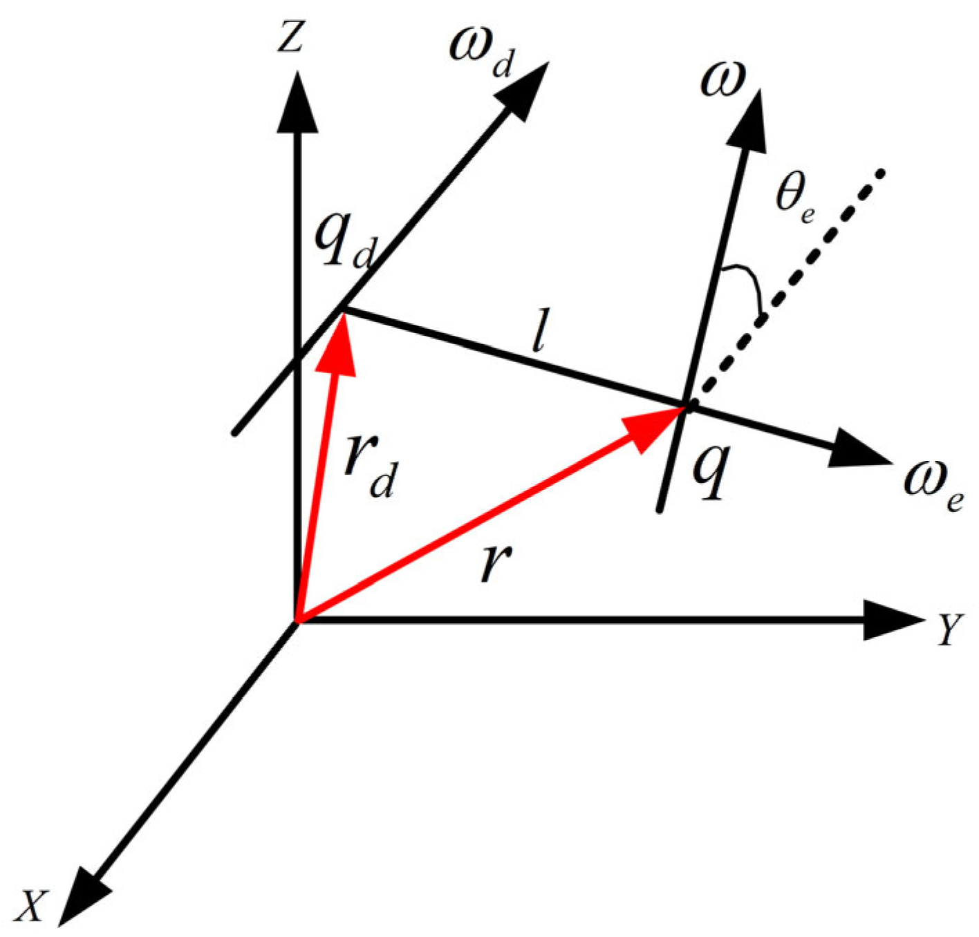
2.4. CTCE Model

The CTCE model is used to calculate the contour error of the AT relative to the ST. As shown in Figure 3, the contour error includes two components: the contour error of TTPT and the contour error of TOT.

In Figure 3, $(P_r,O_r)$ is the ideal tool pose of a certain position on the ST, and $(P_a,O_a)$ is the actual tool pose of the position on the AT. $(P_c,O_c)$ is the tool pose closest to the actual tool pose on the ST. The contour error of TTPT $\overrightarrow{{\epsilon }_p}$ is defined as the distance between the actual tool-tip position $P_a$ and the tool-tip position $P_c$, where position $P_c$ is the closest position to position $P_a$ on the ST. The contour error of TOT ${\epsilon }_o$ is defined as the angle between $O_a$ and $O_c$. In this section, the method developed by Lyu [33] is used to solve the CTCE.

2.4.1. The Solution of the Contour Error of TTPT

As shown in Figure 4, the actual tool-tip position $P_a$ relative to position $P_r$ can be divided into three cases. According to the definition of the contour error of TTPT, the calculation methods can be as follows:

Case 1, use the interpolation segment $\overline{P_{r,(i-1)}{P}_{r,\left(i\right)}}$ before the tool-tip position $P_{r,(i)}$ for calculation;

Case 2, use the tool-tip position $P_{r,(i)}$ for calculation;

Case 3, use the interpolation segment $\overline{P_{r,(i)}{P}_{r,(i+1)}}$ after the tool-tip position $P_{r,(i)}$ for calculation.

Figure 5 shows the geometric relationship between the contour error of TTPT $\overrightarrow{{\epsilon }_p}$ and the vector $p$ of $\overline{P_{r,\left(i\right)}{P}_a}$ in three cases. In cases 1 and 3, the TTPT error is:

$${\overrightarrow{\epsilon }}_p={\epsilon }_x·i+{\epsilon }_y·j+{\epsilon }_z·k=p-p^{\prime }$$

(16)

where $p^{\prime }$ is the projection vector of vector $p$ on line segment $\overline{P_{r,(i-1)}{P}_{r,\left(i\right)}}$ or $\overline{P_{r,(i)}{P}_{r,(i+1)}}$.

$$‖\epsilon ‖=\sqrt{{\epsilon }_x^2+{\epsilon }_y^2+{\epsilon }_z^2}$$

(17)

In case 2, the contour error of TTPT is directly represented by $p$, that is, $\overrightarrow{{\epsilon }_p}=p$, and its value is:

$$‖\epsilon ‖=\sqrt{p_x^2+p_y^2+p_z^2}$$

(18)

2.4.2. The Solution of the Contour Error of TOT

As shown in Figure 6, each tool-tip position on a certain trajectory has its corresponding tool orientation. Tool orientation is a unit vector. If the starting point of the vector is placed at the same coordinate origin, the end-point of the vector will move on a sphere with radius 1, and the moving trajectory is the TOT.

According to the definition of the contour error of TOT, when error ${\epsilon }_o$ is expressed in radians, it is an arc between vector A and vector B, and its value is approximately equal to the chord length corresponding to the arc:

$$\begin{array}{l}{\epsilon }_0 = <O_a,O_c>\\ {\epsilon }_0 \approx \left|O_c-O_a\right|\end{array}$$

(19)

3. Experiment and Results

Integrating the ST model, the AT model and the CTCE model, the DT of the KMC400S U five-axis machine tool (Manufactured by the KEDE Numerical Control Co., Ltd; Dalian, China) is first established, and the S specimen is used as an example to predict the contour error of the S-shaped trajectory offline by using the DT. The predicted results are compared with the measured results. In this way, the correctness of the DT is verified; then, the DT of the DMU50 five-axis machine tool (Manufactured by the DMG MORI AKTIENGESELLSCHAFT; Bielefeld, Germany) is established to study the real-time collection of machine tool data and online real-time prediction of the CTCE during the part machining process.

3.1. The DT of the KMC400S U Five-Axis Machine Tool

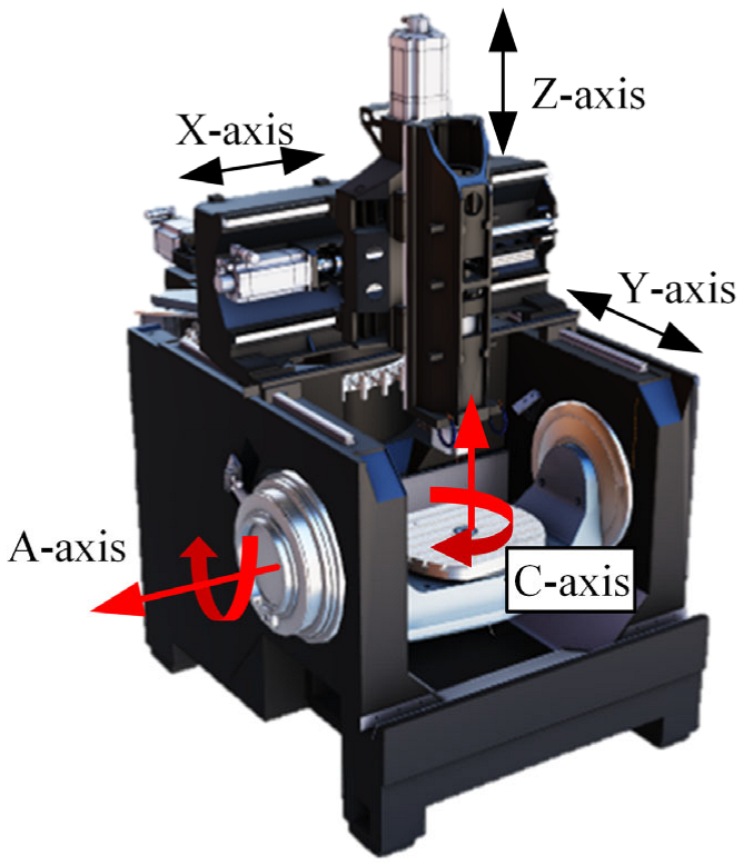
3.1.1. Experimental Equipment and Steps

The experimental machine tool is the Kede KMC400S U vertical milling machining center, as shown in Figure 7. Based on the DT modeling method proposed, the DT of the five-axis machine tool is established. Firstly, the ST model is established through the basic geometric information of the machine tool. Then, 41 geometric errors of the machine tool are measured, and the screw motions of geometric errors are calculated to establish the AT model. Finally, the CTCE model is established according to the method described in Section 2.4.

3.1.2. The ST Model of the KMC400S U Five-Axis Machine Tool

The ST model of the machine tool is established by the method described in Section 2.2. The parameter information of the machine tool is shown in

Table 1. The parameters of the KMC400S U five-axis machine tool.

Parameters	Value
Tool length	150/mm
Origin of machine coordinate system	C-axis control point
Vector from A-axis control point to C-axis control point	(0, −39.9985, −99.9895)
Vector from C-axis control point to center of spindle end	(0, 0, 0)

, and the kinematic chain of the machine tool is shown in Figure 8.

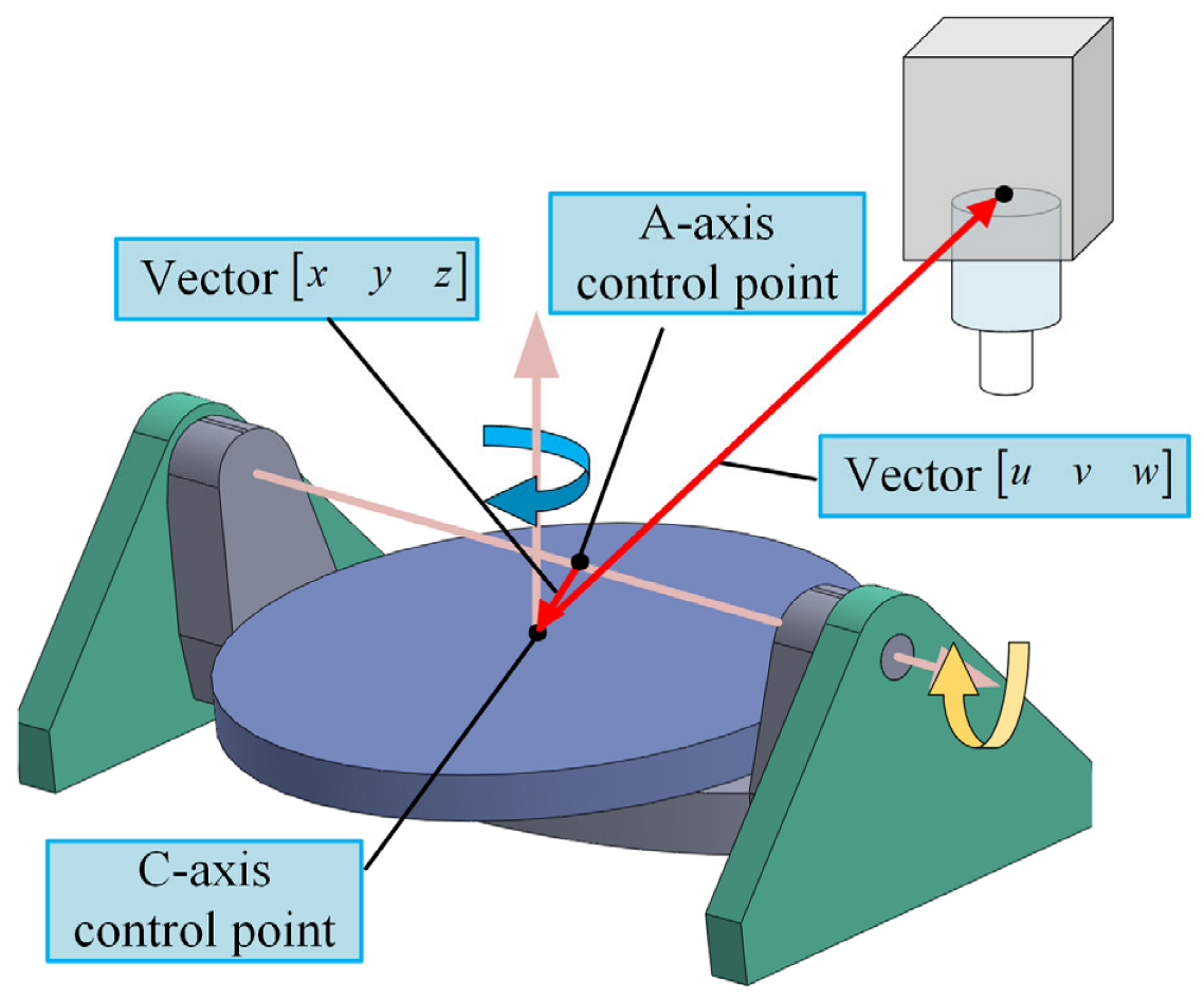
The A-axis control point in

Table 2. The PDGEs of X-axis.

Position /mm	${\mathit{\delta }}_{\mathit{x}\mathit{x}}/\mathbf{mm}$	${\mathit{\delta }}_{\mathit{y}\mathit{x}}/\mathbf{mm}$	${\mathit{\delta }}_{\mathit{z}\mathit{x}}/\mathbf{mm}$	${\mathit{\epsilon }}_{\mathit{y}\mathit{x}}/\mathbf{arcsec}$	${\mathit{\epsilon }}_{\mathit{z}\mathit{x}}/\mathbf{arcsec}$
100	0	0.0034	−0.0055	−0.6	−0.1
80	−0.0002	0.0003	−0.0024	−0.9	0.2
60	−0.0006	0.0013	0.0003	−1.1	0.9
40	−0.0006	0.0033	0.0032	−1.1	0.9
20	−0.0006	0.0045	0.0035	−1.0	1.2
0	−0.0005	0.0048	0.0033	−0.9	1.4
−20	−0.0001	0.0025	0.0020	−1.1	1.5
−40	−0.0001	0.0062	0.0017	−1.5	1.6
−60	−0.0005	0.0086	0.0030	−1.4	1.9
−80	−0.0007	0.0071	0.0047	−1.5	2.1
−100	−0.0007	0.0039	0.0044	−1.9	2.1
−120	0.0004	0.0033	0.0028	−1.9	2.1
−140	0.0016	0.0014	0.0002	−1.8	1.8
−160	0.0020	−0.0011	−0.0022	−1.8	1.8
−180	0.0020	−0.0024	−0.0040	−1.4	1.8
−200	0.0030	−0.0024	−0.0040	−1.5	2.0

is a point located on the rotation axis of the A-axis, which is the coordinate origin of the A-axis rotation coordinate system. Similarly, the C-axis control point is a point on the rotation axis of the C-axis, which is the coordinate origin of the C-axis rotation coordinate system. Figure 9 shows the relative position between the C-axis control point and the A-axis control point and the relative position between the C-axis control point and the center of the spindle end. The vector $(x,y,z)$ is the vector from A-axis control point to C-axis control point in the initial state of the machine tool, and vector $(u,v,w)$ is the vector from C-axis control point to the center of the spindle end in the initial state of the machine tool.

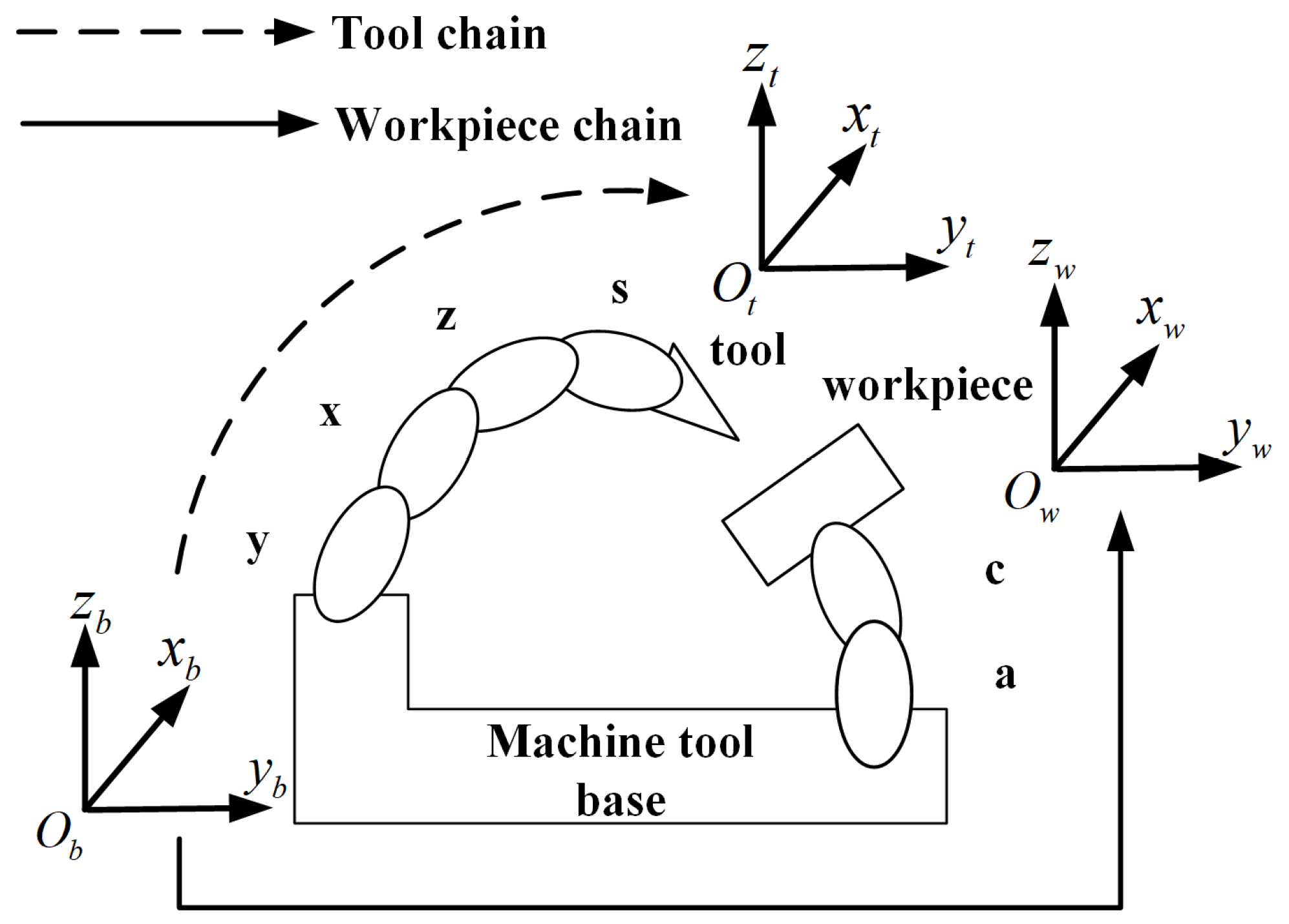
The kinematic chain of the KMC400S U five-axis machine tool is shown in Figure 8. Set the origin of the BCS at the C-axis control point. One side of the workpiece chain successively includes A-axis, C-axis and workpiece, and one side of the tool chain successively includes Y-axis, X-axis, Z-axis and tool. Then, the ST model of the machine tool is obtained from Equations (5)–(8) as:

$$\begin{array}{l}\left[\begin{array}{cc}\begin{array}{c}{P}_x\\ P_y\\ P_z\\ 1\end{array}& \begin{array}{c}{O}_i\\ O_j\\ O_k\\ 0\end{array}\end{array}\right]={\left[g_{bw}(0)\right]}^{-1}{e}^{-{\stackrel{\wedge }{\xi }}_C{\theta }_C}{e}^{-{\stackrel{\wedge }{\xi }}_A{\theta }_A}{e}^{{\stackrel{\wedge }{\xi }}_Y{\theta }_Y}•\\ e^{{\stackrel{\wedge }{\xi }}_X{\theta }_X}{e}^{{\stackrel{\wedge }{\xi }}_Z{\theta }_Z}\left[g_{bt}(0)\right]\left[\begin{array}{cc}\begin{array}{c}0\\ 0\\ 0\\ 1\end{array}& \begin{array}{c}0\\ 0\\ 1\\ 0\end{array}\end{array}\right]\end{array}$$

(20)

1.

Calculation of$\left[g_{bw}(0)\right]$and$\left[g_{bt}(0)\right]$;

In Equation (20), $\left[g_{bw}(0)\right]$ is the offset of the WCS relative to the BCS in the initial state of the machine tool, which is usually the value of G54 set in the CNC system, assuming that the value of G54 is $\left(\begin{array}{ccc}G{54}_x& G{54}_y& G{54}_z\end{array}\right)$; $\left[g_{bt}(0)\right]$ is the offset of the TCS relative to the BCS, and the offset value is the tool length $L_{tool}$.

$$\left[g_{bt}(0)\right]=\left[\begin{array}{cccc}1& 0& 0& 0\\ 0& 1& 0& 0\\ 0& 0& 1& -L_{tool}\\ 0& 0& 0& 1\end{array}\right]\left[g_{bw}(0)\right]=\left[\begin{array}{cccc}1& 0& 0& G{54}_x\\ 0& 1& 0& G{54}_y\\ 0& 0& 1& G{54}_z\\ 0& 0& 0& 1\end{array}\right]$$

(21)

2.

Calculation of screw motion ${\mathrm{e}}^{\stackrel{\wedge }{\xi }\theta }$ of each axis;

According to Equation (1), the screw motions of translational axes are calculated as:

$$\begin{array}{l}{e}^{\stackrel{\wedge }{{\xi }_x}x}=\left[\begin{array}{cc}{I}_{3\times 3}& v_x{\theta }_x\\ 0_{1\times 3}& 1\end{array}\right]=\left[\begin{array}{cccc}1& 0& 0& x\\ 0& 1& 0& 0\\ 0& 0& 1& 0\\ 0& 0& 0& 1\end{array}\right]\\ e^{\stackrel{\wedge }{{\xi }_y}y}=\left[\begin{array}{cc}{I}_{3\times 3}& v_y{\theta }_y\\ 0_{1\times 3}& 1\end{array}\right]=\left[\begin{array}{cccc}1& 0& 0& 0\\ 0& 1& 0& y\\ 0& 0& 1& 0\\ 0& 0& 0& 1\end{array}\right]\\ e^{\stackrel{\wedge }{{\xi }_z}z}=\left[\begin{array}{cc}{I}_{3\times 3}& v_z{\theta }_z\\ 0_{1\times 3}& 1\end{array}\right]=\left[\begin{array}{cccc}1& 0& 0& 0\\ 0& 1& 0& 0\\ 0& 0& 1& z\\ 0& 0& 0& 1\end{array}\right]\end{array}$$

(22)

Among them, $x,y,z$ are the SPs of each translational axis in the MTCS.

Then, calculate the screw motion ${\mathrm{e}}^{\stackrel{\wedge }{\xi }{\theta }_c}$ of the C-axis according to Equation (2), where ${\theta }_c$ is the SP of the C-axis in the MTCS, ${\omega }_c={\left[\begin{array}{ccc}0& 0& 1\end{array}\right]}^T$, $q_c$ is any point on the C-axis, select $q_c$ as the C-axis control point, $q_c={\left[\begin{array}{ccc}0& 0& 0\end{array}\right]}^T$, so ${\mathrm{e}}^{\stackrel{\wedge }{\xi }{\theta }_c}$ is calculated as:

$${\mathrm{e}}^{\stackrel{\wedge }{{\xi }_c}C}=\left[\begin{array}{cccc}\cos {\theta }_c& -\sin {\theta }_c& 0& 0\\ \sin {\theta }_c& \cos {\theta }_c& 0& 0\\ 0& 0& 1& 0\\ 0& 0& 0& 1\end{array}\right]$$

(23)

Finally, calculate the screw motion ${\mathrm{e}}^{\stackrel{\wedge }{\xi }{\theta }_a}$ of the A-axis according to Equation (2), where ${\theta }_a$ is the SP of the A-axis in the MTCS, ${\omega }_a={\left[\begin{array}{ccc}1& 0& 0\end{array}\right]}^T$, $q_a$ is any point on the A-axis, select $q_a$ as the A-axis control point, according to the information in Table 1, $q_a={\left[\begin{array}{ccc}0& 39.9985& 99.9895\end{array}\right]}^T$, so ${\mathrm{e}}^{\stackrel{\wedge }{\xi }{\theta }_a}$ is calculated as:

$${\mathrm{e}}^{\stackrel{\wedge }{{\xi }_a}A}=\left[\begin{array}{cccc}1& 0& 0& 0\\ 0& \cos {\theta }_a& -\sin {\theta }_a& 99.9895\sin {\theta }_a+39.9985(1-\cos {\theta }_a)\\ 0& \sin {\theta }_a& \cos {\theta }_a& 99.9895(1-\cos {\theta }_a)-39.9985\sin {\theta }_a\\ 0& 0& 0& 1\end{array}\right]$$

(24)

Substituting the screw motion of each axis obtained by the above calculation into Equation (20), the ST model of the KMC400S U five-axis machine tool is established.

3.1.3. The AT Model of the KMC400S U Five-Axis Machine Tool

The AT model of the machine tool is established according to the method described in Section 2.3.

The KMC400S U five-axis machine tool has 41 geometric errors. Among them, the 21 geometric errors of the translational axes are measured by the laser interferometer (18 of which can be measured except 3 rolling errors), and the 20 geometric errors of the rotary axes are measured by R-Test, as shown in Figure 10.

The measured geometric error data are characterized as polynomials or constants, and then expressed in the form of an error twist. Taking the angular error ${\epsilon }_{yx}$ of the X-axis as an example, as shown in Figure 11, through the 3rd-order fitting, it is first characterized as a function expression that changes with the position of the X-axis.

The function of the error ${\epsilon }_{yx}$:

$${\epsilon }_{yx}=-1.79\times {10}^{-7}{x}^3-1.23\times {10}^{-5}{x}^2+0.006x-1.141$$

(25)

The angular error ${\epsilon }_{yx}$ is represented by the error twist, as shown in Figure 12, $q$ is any point on the X-axis, which is selected as the origin of the X-axis coordinate system.

According to Equation (12), the error twist of the error ${\epsilon }_{yx}$ is:

$${\xi }_e={\left[\begin{array}{cc}\begin{array}{c}0\\ 0\\ 0\end{array}& \begin{array}{c}0\\ 1\\ 0\end{array}\end{array}\right]}^T$$

(26)

Substitute the error twist of error ${\epsilon }_{yx}$ into Equation (2), and obtain its screw motion as:

$${\mathrm{e}}^{\stackrel{\wedge }{\xi }\theta }=\left[\begin{array}{cccc}1& 0& {\epsilon }_{yx}& 0\\ 0& 1& 0& 0\\ -{\epsilon }_{yx}& 0& 1& 0\\ 0& 0& 0& 1\end{array}\right]$$

(27)

Similarly, the screw motions of other geometric errors are obtained. According to Equations (13)–(15), the AT model of the KMC400S U five-axis machine tool is:

$$\begin{array}{l}\left[\begin{array}{cc}\begin{array}{c}{P}_x{}^e\\ P_y{}^e\\ P_z{}^e\\ 1\end{array}& \begin{array}{c}{O}_i{}^e\\ O_j{}^e\\ O_k{}^e\\ 0\end{array}\end{array}\right]={\left[g^e{}_{bw}(0)\right]}^{-1}{e}^{-{\stackrel{\wedge }{{\xi }^e}}_C{\theta }_C{}^e}{e}^{-{\stackrel{\wedge }{{\xi }^e}}_A{\theta }_A{}^e}{e}^{{\stackrel{\wedge }{{\xi }^e}}_Y{\theta }_Y{}^e}•\\ e^{{\stackrel{\wedge }{{\xi }^e}}_X{\theta }_X{}^e}{e}^{{\stackrel{\wedge }{{\xi }^e}}_Z{\theta }_Z{}^e}\left[g^e{}_{bt}(0)\right]\left[\begin{array}{cc}\begin{array}{c}0\\ 0\\ 0\\ 1\end{array}& \begin{array}{c}0\\ 0\\ 1\\ 0\end{array}\end{array}\right]\end{array}$$

(28)

where the screw motion of each axis and the values of $\left[g^e{}_{bw}(0)\right]$ and $\left[g^e{}_{bt}(0)\right]$ are the same as those in the ST model.

3.2. The Offline Prediction Process of Contour Error

The input data of the DT proposed are SP data and LEDP data. The sampling frequency of these two channels is high (the same as the interpolation frequency of the CNC system, 500Hz). In addition, for the five-axis machine tool, the data of 10 channels need to be collected synchronously. In the case of the multi-channel and high-sampling frequency, using data real-time acquisition methods such as OPCUA is easy to cause data synchronization disorder. Therefore, in order to verify the correctness of the establishment method of DT, an off-line prediction verification scheme is designed.

3.2.1. The AT Model of the KMC400S U Five-Axis Machine Tool

The ruled surface A of an S-shaped edge strip shown in Figure 13 is taken as the processing object. The prediction process is shown in Figure 14. Firstly, the S-shaped edge strip is processed on the KMC400S U five-axis machine tool, and the SP and LEDP data during the processing are collected offline. Secondly, input the SP data and LEDP data into the DT of the machine tool, and predict the contour error of the S-shaped trajectory.

In order to verify the correctness of the contour error of the S-shaped trajectory predicted by the DT, the Coordinate Measuring Machine (CMM) is used to measure the ruled surface A to obtain the measured trajectory for comparison with the predicted contour error.

3.2.2. Collection of SP and LEDP Data

The data of SP and LEDP in the process of finishing the S-shaped trajectory are collected through G237 and G238 commands in Kede CNC system. The code format is shown in Figure 15. The G237 and G238 commands mean the data acquisition is starting and stopping, respectively. The sampling period of the data is 2 ms, which is the same as the interpolation period of the CNC system. The collected data of the SP and LEDP of the five axes are shown in Figure 16 and Figure 17.

3.2.3. Predicted and Measured Results of Contour Error

Inputting the collected SP and LEDP data into the DT of the KMC400S U five-axis machine tool, the ST and the AT are synthesized as shown in Figure 18. The predicted contour error is shown in Figure 19.

In order to verify the correctness of the predicted contour error, the CS100 CMM is employed to measure a trajectory of the ruled surface A. A total of 900 points are measured on the Measured Trajectory (MT) is shown with a black line in Figure 20. The ST and AT in this section are also shown in this figure with blue and red lines for comparison. The accuracy of the CMM is $1.5\mu m+L(mm)/350$, where $L$ is the measurement length.

The ST in Figure 20 shows a preset S-shape, which verifies the ST model. There is a certain deviation between the AT and the ST, which is reflected in the influence of geometric errors and tracking errors. The MT measured by CMM is approximately the same as the AT predicted by DT, and both curves reflect some peak characteristics, which indicates the correctness of the established DT.

However, the AT predicted by DT is not exactly coincident with the MT measured by CMM, and the trend of the two curves and the error of each point are different to some extent, as shown in Figure 21. The reason is that the error of the AT only considers the geometric errors and the tracking errors, whereas the error of the MT also includes the influence of factors such as principle error, dynamic error outside servo-loop and cutting deformation. These factors need to be considered in the future to further correct the DT of the machine tool.

3.2.4. Analysis of Calculation Time of Contour Error

MATLAB software (Published by The MathWorks; Natick, Massachusetts, USA) is used to write the algorithm of DT of the KMC400S U five-axis machine tool. The data of SP and LEDP during the finishing the ruled surface A are inputted to the DT; then, record the time required to calculate the contour error. The sampling frequency of the data SP and LEDP is 2 ms, the sampling time is 39.358s, and data point (SP) is 19,680 in total.

Running the program, the recording time for calculating the contour error for all the positions is about 28.8864s. For every position, the average calculated time of the contour error is about 1.4 ms. The calculation speed is higher than the sampling frequency, which can meet the real-time requirements of DT in principle.

However, according to the CTCE model, the contour error is calculated by searching the tool pose closest to the actual tool pose on the ST. Therefore, it is necessary to synthesize a short trajectory before the calculation of the contour error. The tool poses closest to the actual tool pose on the ST is within about 10 tool-tip positions before and after the tool-tip position on the ST corresponding to the tool-tip position on the AT. Therefore, when the sampling frequency is 2ms, the calculation of the contour error will have a lag of about 40ms.

3.3. The Offline Prediction Process of Contour Error

By establishing the DT of the KMC400S U five-axis machine tool, the offline prediction of the contour error is realized, which verifies the correctness of the proposed method. However, real-time data is the premise of the operation of the DT. Therefore, this paper uses the OPC UA protocol to obtain the SP and LEDP data in real time during the machining process of the machine tool. Taking the DMU50 five-axis machine tool as an example, its CNC system supports data collection through the OPC UA protocol. Similar to the establishment method of the DT of the KMC400S U five-axis machine tool, it will not be repeated here. According to the proposed method, the DT of the DMU50 five-axis machine tool is established to study the real-time prediction of contour error.

This paper uses the OPC UA toolkit of Labview software (Published by National Instruments; Austin, Texas, USA) to connect with the OPC UA server of the Siemens CNC system (Published by SIEMENS AG; Berlin, Germany) to realize real-time data acquisition. The data acquisition process based on Labview software is as follows: First, you need to activate the OPC UA server license installed inside the Siemens CNC system. After the OPC UA server license is activated, use Labview’s OPC UA toolkit to create an OPC UA client, and connect the OPC UA server and Labview through the Ethernet interface X127. The client adopts the subscription mode and selects the data variables to be subscribed. When the machine tool runs the program, the server will continuously ask the CNC system to detect whether the variables subscribed by the client have changed. When the change is detected, it will actively send data to the client. Then, since the algorithms used to establish the DT of the machine tool are all written in Matlab, the script function in Labview is used to integrate the program in Matlab into Labview, and the program in Matlab can be called in Labview. Finally, through the graphical function in Labview, the real-time display of the real-time prediction result of the CTCE can be realized.

As shown in Figure 22, the G code of the spatial circular trajectory is run on the machine tool, and the data is collected in real time and the contour error is predicted in real time.

As shown in Figure 23, while running the space circular trajectory, the data acquisition program in Labview can collect the SP and LEDP data of each axis in real time, and visualize them in real time in the graphical interface. The collected data is used to synthesize the ST and the AT and calculate the CTCE through the Matlab script function, and the results are displayed in real time.

At this point, based on the OPC UA protocol, the real-time prediction of the CTCE can be realized during the operation of the machine tool, and the results can be displayed in real time.

However, the data collection based on the OPC UA protocol has a sampling frequency of up to 10HZ, while the data collection based on the edge can have a sampling frequency of up to 500 HZ, and the collected data is more complete. Therefore, subsequent research can use edge to study the real-time prediction of CTCE.

4. Conclusions and Future Works

This paper proposes a DT modeling method of five-axis machine tools for predicting CTCE caused by tracking errors and geometric errors. The DT consists of three parts: the ST model, the AT model and the CTCE model.

For the establishment of the DT of a specific machine tool, it is necessary to know the basic geometric information of the machine tool (tool length, kinematic chain information, etc.), while the 41 geometric errors need to be measured in advance.

During or before the machining of the part, collect the SP and LEDP data of each axis, and input them into the DT of the machine tool, to realize the offline or real-time prediction of the CTCE.

In the future, further research will be made on the real-time performance of DT of machine tools based on edge.