Systematic Parameter Estimation and Dynamic Simulation of Cold Contact Fermentation for Alcohol-Free Beer Production

Abstract

Global demand for Low-Alcohol Beer (LAB) and Alcohol-Free Beer (AFB) has surged due to flavor attributes, health benefits, and lifestyle changes, prompting efforts for process intensification. This paper aims to offer a detailed modelling basis for LAB manufacturing study and optimisation. A first-principles dynamic model for conventional beer manufacturing has been re-parameterized and used for dynamic simulation of Cold Contact Fermentation (CCF), an effective LAB and AFB production method, with concentrations tracked along plausible temperature manipulation profiles. Parameter estimation is pursued using industrial production data, with a detailed local sensitivity analysis portraying the effect of key parameter variation on sugar consumption, ethanol production, and key flavor component (ethyl acetate and diacetyl) evolution during (and final values after) CCF. Ethyl acetate (esters in general) affecting fruity flavors emerge as most sensitive to CCF conditions.

1. Introduction

1.1. Low-Alcohol Beer (LAB) and Alcohol-Free Beer (AFB)

Beer brewing is an ancient practice [1], ingrained in local traditions of many cultures worldwide. Though resulting from agricultural village surpluses, the modern brewing industry has expanded its manufacturing and commercial presence to meet vast global consumption [2]: recent estimates by the World Health Organization (WHO, 2014) confirm that beer is the second most imbibed (top alcoholic) beverage worldwide [3]. This gradual progression from rural artisanal activity to modern industrial complex is illustrated by global production metrics, with 1.95·10¹¹ L of beer produced in 2017 [4]. From a processing viewpoint, grouping beverages under the term ‘beer’ is a deliberate simplification, as it encompasses a multitude of different products of varying alcohol content [5], from Pilsners and Lagers (known as “bottom fermenting”) to Weissbiers and Ales (known as “top fermenting”) [6]. Different classifications and models [7] are based on alcohol strength (i.e., concentration). The range starts from Alcohol-Free Beer (AFB) at 0–1.2% (v/v) and moves to Low-Alcohol Beer (LAB) at 1.2–3% (v/v) before the classification of the vast majority of standard brew concentrations of 3–6% (v/v) [8,9].

The classification of AFB and LAB has a remarkable historical backdrop, with origins in the United States Prohibition era (1919–1933), but also as a reaction to raw material shortages during World War I and II (1939–1945) [9]. Global demand for zero-/low-alcohol products has surged recently, with an estimated 80% consumption increase from 2007 to 2012, in which it reached 2.2·10⁹ L yr⁻¹ [10]. Several explanations from a social perspective have been presented for this clear trend in beer sales, including stringent legal restrictions on consumption and wider awareness of moderation benefits. Recent efforts by beverage corporations to penetrate countries and access markets in which alcohol consumption is forbidden for religious reasons also seems to have had a significant contribution [9]. Health benefits of increased AFB and LAB consumption in contrast to standard alcoholic beverages are substantial, as beneficial beer (antioxidant, anti-cancer, and phytoestrogen) components are retained at remarkably lower energy content (e.g., LAB has a 60.7% lower calorie content vs. pale ale) [11,12].

This differentiation among beer types is also critical in the different processing methods required to achieve different flavor profiles and strengths: even within the narrow AFB ethanol concentration, various production methods exist, categorized as either physical (post-processing) or biological (pre-processing) [8]. The former focus on dealcoholization via, e.g., distillation, adsorption, or dialysis: they require additional capital expenditure, being more expensive at production scale [10,13]. The latter alter the fermentation step itself via special yeast strains, yeast immobilization, CCF, or arrested fermentation, resulting in published ethanol concentration ranges from 0.02% (v/v) and up [11,12,13,14,15].

The most promising of these methods is Cold Contact Fermentation (CCF), also known as Cold Contact Process (CCP), which combines low fermentation temperatures (0–8 °C) and contact times of 24–100 h [16,17,18,19]. First proposed by Schur in 1983 [16], this batch method enjoys wide industrial use towards high AFB volumes [17,18]. Nevertheless, it may induce flavor deficiencies due to high levels of undesirable compounds, e.g., methional and Strecker aldehydes (2- and 3-methylbutanal) [17,18,19].

Laboratory-scale CCF research has been covered in the literature since inception [8,9], but CCF dynamic modeling has not yet received interest commensurate with beverage demand, especially compared with dynamic modeling and optimization success for ‘warmer’ ale and lager (6–22 °C) brewing [20,21,22,23,24]. We thus aim to pave the way for robust modeling platforms and higher industrial process efficiency.

Increased market LAB/AFB demand and health benefits vs. higher-alcohol beer are key drivers. This paper aims to establish a CCF modeling basis for process intensification as experimental work in the beer industry incurs high costs and implies use of process equipment for (risky) manipulations.

The latter may arise from the need for introducing new products (e.g., LAB/AFB), or implementing process improvements for existing products. This opportunity cost increases with production scale, as bigger plant facilities use larger equipment and thus incur a higher subsumed downtime cost. Revenue (thus, profit) to be maximized is a function of product sales, but engineering upgrades can have a critical effect on throughput. Evaluation of improvements via computational methods (e.g., process modeling) holds value for CCF, especially in light of increased global LAB/AFB consumption. Our goal is to probe CCF process potential using model reparameterization and sensitivity analyses.

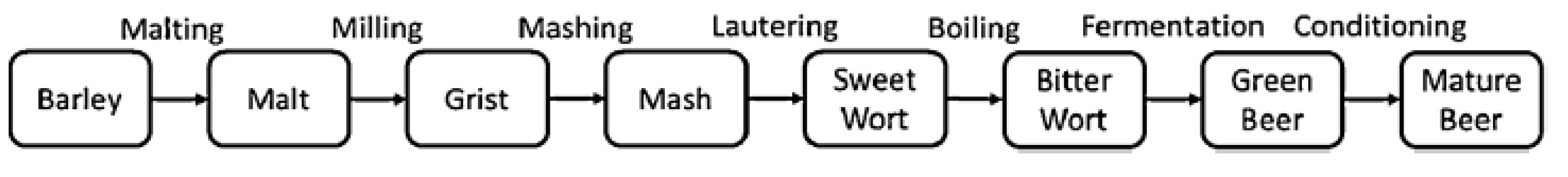
1.2. Beer Manufacturing

Detailed understanding of beer manufacturing process steps (Figure 1) is key for appreciating how fermentation variants/specifications (e.g., CCF vs. warm fermentation) induce vast upstream and downstream changes in the seemingly simple interplay of barley malt, hops, yeast, and water [25].

Beer manufacturing starts with the malting process: barley is converted to malt by kernel wetting and induced sprouting, simulating natural grain germination. The germinated embryo here secretes natural plant hormones (gibberellins) inducing production and activation of key enzymes (especially amylases) which are crucial towards hydrolyzing the endosperm starch later, during mashing [12]. Malt kilning to remove water follows, before degermination and storage until actual brewing use [5].

The brewing process commences with milling: the malt mixture is comminuted to grist, and the latter is added to water and mashed under heating, towards starch liquefaction and saccharification. The mash is then fed into the lauter tun, to separate the liquid wort from spent grist solids: this is the ‘first wort’ extraction, followed by subsequent extractions (‘last runnings’) of inferior composition. The liquid wort is transferred to a kettle and boiled to kill bacteria, remove dimethyl sulfide (DMS), induce flavor and color formation (Maillard melanoidin production), and cause enzyme degradation. This opportune point also the serves secondary feed (hops, corn syrup) addition, as per brand recipes; wort boiling ensures isomerisation of hop alpha acids, as 99% of beers are brewed with hops [5]. The mixture is subsequently transferred to a whirlpool for precipitated hop and protein (‘hot trub’) removal, then to a cooling heat exchanger (as low as 0–1 °C for CCF) before fermentation [2,8].

The bitter, cooled wort from the boiling process is fed to fermentors with yeast (‘pitching’) and a small amount of air to promote initial biomass growth [25] and subsequent fermentable sugar consumption by yeast towards the production of beer, the very purpose of a fermentation phase [5]. Temperature and batch duration are pivotal, as they govern hundreds of chemical reactions and kinetics, driving flavor creation [26]. For the various cases for producing alcoholic beer via warm fermentation, temperatures range from 6 to 22 °C and total contact period of 5–21 days. The CCF method employs contact times of 24–100 h at temperatures of 0–8 °C, to inhibit ethanol formation while maintaining adequate flavor component formation levels. The resulting ‘green beer’ is washed by CO₂ bubbling to remove aldehydes before maturation and storage in casks, barrels, or bottles [1,2].

1.3. Organoleptic Constituents and Sensory Characteristics

Beer flavor is broader than taste, as the sum of perceptions from sensory element stimulation at the entrance of alimentary and respiratory tracts [25] also includes odor, aroma, and mouthfeel [26]. Key AFB batch flavor (quality) metrics include ethanol, pH, and residual (unfermented) sugar levels. However, an AFB deficiency is associated with excessive sweetness, worty off-flavors, bitterness, and possible absence of desirable aroma [27]. Chemical complexity thus poses further complications, as even acceptable physicochemical properties do not always imply satisfactory product taste [28]. Flavor is also perplexed by synergistic or suppressive phenomena due to other compounds: a mixture of, e.g., two or more aldehydes (all below thresholds) can still have a perceivable flavor effect [29,30].

Chief chemicals inducing undesirable beer flavor include Vicinal Diketones (VDKs), e.g., diacetyl (2,3-butanedione) and 2,3-pentanedione [31]. Other aldehydes are also crucial, e.g., 2-methylbutanal, 3-methylbutanal, furfural, acetaldehyde, isobutyraldehyde, 2-phenylacetaldehyde, methional, and 3-methylthiopropionaldehyde [32]. Worty off-flavors emerging from CCF are due to 2-methylbutanal, 3-methylbutanal, and 3-methylthiopropionaldehyde [17,18,19]. Higher (fusel) alcohol (e.g., propanol, butanol) levels must also be controlled, because their high concentration is strongly correlated with hangover effects. Esters ensure desirable beer flavor profiles (e.g., fruitiness): ethyl acetate, ethyl caproate, isoamyl acetate, ethyl caprylate, ethyl hexanoate, and phenyl ethyl acetate are critical [33].

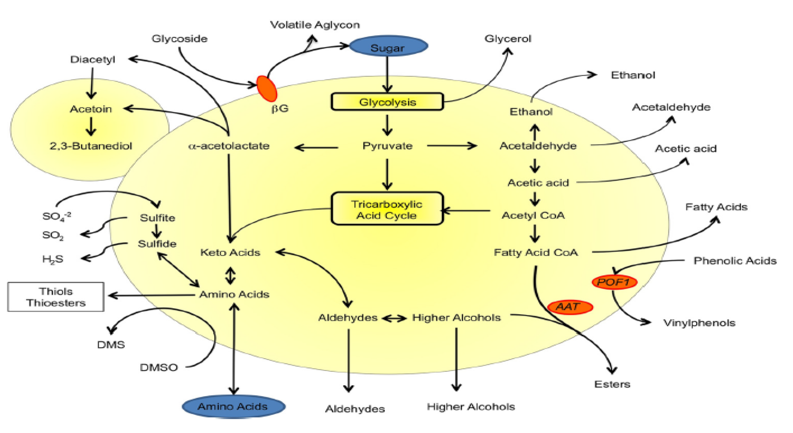
1.4. Metabolic and Non-Metabolic Pathways

Several different types of yeast are used in beer brewing, though the most popular genus across all methods is Saccharomyces, with strains such as Saccharomyces pastorianus (formerly Saccharomyces carlsbergensis) and Saccharomyces cerevisiae (brewer’s yeast) mostly cited for CCF processing [34,35]. The most important reaction occurring over the course of any fermentation process is the conversion of the sugars in wort to ethanol and carbon dioxide. This is represented by the Gay-Lussac equation:

C₆H₁₂O₆ → 2C₂H₅OH + 2CO₂, ΔH = −68.4 kJ

(1)

The reaction is overall exothermic, as clearly denoted by the negative sign of reaction enthalpy. Equation (1) is a clear simplification that does not portray the complex phenomena during the fermentation process: these are distinguished into metabolic (intracellular) and non-metabolic (extracellular) [13]. Figure 2 presents a high-level overview of significant metabolic phenomena during beer fermentation.

Carbonyls are formed via metabolic pathways (e.g., Strecker aldehyde degradation of amino acids, and lipid degradation), as well as by the non-metabolic pathway of Maillard reactions, which yield a vast variety of products [36,37]. Furfural (one of the principal products formed therein) can be used as a heating load indicator for beer at various process stages, as its concentration increases throughout brewing and through maturation [29]. Esters are produced in part by the transesterification of acetyl-coenzyme A and are tightly linked to lipid metabolism (Figure 2) [33,36]. Many pathways are inter-connected (e.g., Maillard reactions generate α-dicarbonyls, while Strecker degradation consume them), showcasing the complexity of this challenging biochemical system vs. industrial manipulation goals.

2. Methodology

2.1. Mathematical Modeling of Fermentation

Beer fermentation is both nonlinear and complex, with its modeling and simulation described as a time-consuming task [2,20,21,22,23,24,31,38,39,40]. Though several mechanisms for enzyme activity exist, Michaelis–Menten and Monod kinetics are the most useful in the present effort. Michaelis–Menten kinetics represent the formation of a product (P_r) resulting from the enzymatic (E) linking with a substrate (S_r), through the reversible formation of an intermediate (SE), as per the following reactions:

$$S_{\mathrm{r}}+E\underset{k_{\mathrm{a}},k_{\mathrm{b}}}{\iff }\mathit{SE}\stackrel{k_{\mathrm{c}}}{\Rightarrow }{E+P}_{\mathrm{r}}$$

(2)

Here, k_b and k_c represent the rate constant for the corresponding forward reactions at each step and k_a denotes the reverse reaction rate constant. The rate of product formation, r_P, is expressed as a ratio:

$$r_{\mathrm{p}}=\frac{k_{\mathrm{c}}{C}_{\mathrm{S}}{C}_{\mathrm{ENZ}}^0}{K_{\mathrm{M}}{+C}_{\mathrm{S}}}$$

(3)

where C_S and $C_{\mathrm{ENZ}}^0$ mark substrate and initial enzyme concentrations, respectively. The variable K_M is the Michaelis–Menten constant = k_a/k_b. While enzymes are chemical substances produced by yeast to catalyze chemical reactions, biomass evolution itself can be described by the Monod equation:

$$r=\frac{r_{\mathrm{m}}{C}_{\mathrm{S}}}{k_{\mathrm{SS}}{+C}_{\mathrm{S}}}$$

(4)

where r is the specific biomass growth rate, r_m is its maximum value, and k_SS is the Monod constant.

Beer fermentation process modeling with explicit kinetics only emerged a few decades ago, rapidly gaining attention after the pioneering computational study of Engasser et al. in 1981 [38]. Process simulation efforts have however not been extended to CCF, with most experimental work at laboratory scale [9]. A chronological review of notable peer-reviewed advances on beer fermentation experiments, modeling, simulation, and optimization since 1981 was recently published [40].

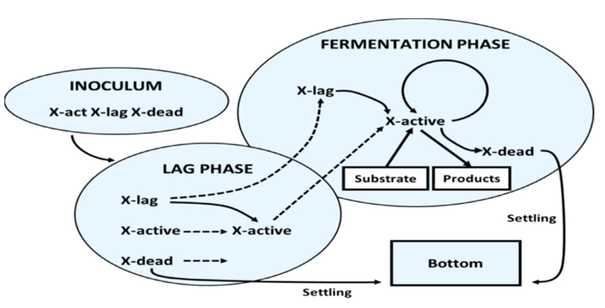
2.2. Model Description

The de Andrés-Toro et al. model considers five state variables: sugar concentration (C_S), ethanol concentration (C_E), total suspended biomass concentration (X_S), ethyl acetate concentration (C_EA), and diacetyl concentration (C_DY) [41]. The total biomass in a fermentation system comprises three entities, active (X_A), latent/lag (X_L), and dead (X_D) biomass, without conservation constraints. Parameters were estimated from concentration trajectories obtained via several isothermal experiments performed at T = 8, 12, 16, 20, and 24 °C, using wort and yeast from Cruzcampo Breweries (Madrid, Spain) [41,42]. Beer fermentation is therein divided in two consecutive (lag and actual fermentation) phases. At the onset of brewing, there is no fermentation. During the lag phase, only dead cell settling and lag cell activation occurs: once the latter reaches 80%, both cell growth and fermentation commence. Thereafter, all four phenomena (settling, activation, growth, and fermentation) occur simultaneously until completion, followed by dilution, fresh (‘green’) beer maturation, and final packaging (Figure 3).

The transition from lag to active cells is implicit in the model and does not require the addition of a secondary model operation (no explicit additional ‘switch’ is included in code implementation). Fermentation can be represented via DAE of ODEs differential equations governing sugar consumption, biomass and ethanol production, and flavor components formation as well as the corresponding Arrhenius expression linked to each of these component specific rates. All these equations are either a function of fermenter temperature (T), fermentation time (t), or both variables.

Experiments by de Andrés-Toro et al. allowed determination of the proportions of each type of cell in the fermenter. Though typically observed as lower in industrial breweries than represented in this model, the proportion of dead cells in the inoculum (X_inc) was 50%, while the remaining 50% of the inoculum comprises 48% lag cells and 2% active cells. This yeast mass balance can be written as:

$$0{.02X}_{\mathrm{inc}}+0{.48X}_{\mathrm{inc}}{=X}_{\mathrm{D}}\left(t=0\right)=0{.5X}_{\mathrm{inc}}$$

(5)

where 0.02X_inc is the proportion of active cells, X_A, in the inoculum and 0.48X_inc is the proportion of lag cells in the inoculum, X_L. After the initial inoculation, the yeast, X_S, is suspended in the wort; the time-dependent biomass concentration comprises all (lag, active and dead) cells. This is denoted as:

$$X_{\mathrm{S}}\left(t\right){=X}_{\mathrm{A}}\left(t\right){+X}_{\mathrm{L}}{\left(t\right)+X}_{\mathrm{D}}\left(t\right)$$

(6)

The rate of conversion of lag cells to active cells is also considered in the model according to:

$$\frac{{\mathrm{d}X}_{\mathrm{L}}}{\mathrm{d}t}{=-\mu }_{\mathrm{L}}{X}_{\mathrm{L}}$$

(7)

where μ_L is the specific rate of lag cell activation, an Arrhenius-type exponential of temperature [41].

Active cells do not multiply in fermentation, but come from cell activation from the lag phase:

$$\frac{{\mathrm{d}X}_{\mathrm{A}}}{\mathrm{d}t}=-\frac{{\mathrm{d}X}_{\mathrm{L}}}{\mathrm{d}t}{, t < t}_{\mathrm{L}}$$

(8)

where t_L is the duration of the fermentation lag phase, in which no cell deterioration is not considered.

Cell death occurs as expired cells settle out of the suspension to the vessel bottom, according to:

$$\frac{{\mathrm{d}X}_{\mathrm{D}}}{\mathrm{d}t}{=\mu }_{\mathrm{SD}}{, t < t}_{\mathrm{L}}$$

(9)

where μ_SD is the dead cell settling rate, a function of both fermentation temperature and duration. The rate of cell suspension is proportional to the dead cell concentration rate of change, according to:

$$\frac{{\mathrm{d}X}_{\mathrm{S}}}{\mathrm{d}t}=-\frac{{\mathrm{d}X}_{\mathrm{D}}}{\mathrm{d}t}$$

(10)

Dead cells settle, thus continuously removed from active cells in the fermentation broth according to:

$$\frac{{\mathrm{d}X}_{\mathrm{S}}}{\mathrm{d}t}{=\mu }_{\mathrm{x}}·X_{\mathrm{A}}{ - \mu }_{\mathrm{SD}}·X_{\mathrm{D}}, t \ge { t}_{\mathrm{L}}$$

(11)

where μ_x is the specific cell growth rate. Active cell concentration is governed by three distinct contributions for active cell growth, active cell death and latent (lag) cell activation, according to:

$$\frac{{\mathrm{d}X}_{\mathrm{A}}}{\mathrm{d}t}{=\mu }_{\mathrm{x}}·X_{\mathrm{A}}{ - \mu }_{\mathrm{DT}}·X_{\mathrm{A}}{+\mu }_{\mathrm{L}}·X_{\mathrm{L}}, t \ge { t}_{\mathrm{L}}$$

(12)

where μ_DT is the specific cell death rate. Biomass activity and availability drives fermentation success, so Equation (12) links cell growth, activation, and death state variables and rates clearly throughout a batch.

Cell death, aside of Equations (10) and (11), is a function of dead cell settling and active cell death, according to:

$$\frac{{\mathrm{d}X}_{\mathrm{D}}}{\mathrm{d}t}{=-\mu }_{\mathrm{SD}}·X_{\mathrm{D}}{+\mu }_{\mathrm{DT}}·X_{\mathrm{A}}, t \ge { t}_{\mathrm{L}}$$

(13)

Substrate (sugar) consumption is considered proportional to active cell concentration, according to:

$$\frac{{\mathrm{d}C}_{\mathrm{S}}}{\mathrm{d}t}{=-\mu }_{\mathrm{S}}·X_{\mathrm{A}}$$

(14)

where μ_S is the specific substrate consumption rate. The rate of change in sugar concentration in the fermenter is a function of sugar consumption by the active biomass. Ethanol formation is also a key component of this system, also considered proportional to active cell concentration, according to:

$$\frac{{\mathrm{d}C}_{\mathrm{E}}}{\mathrm{d}t}{=f}_{\mathrm{inhib}}·{\mu }_{\mathrm{E}}·X_{\mathrm{A}}$$

(15)

where f_inhib denotes the inhibition factor, portraying the detrimental effect of high ethanol concentrations on biomass (yeast) proliferation (μ_E is the specific ethanol production rate). The biomass hence reacts to reduce the production of ethanol and promote cell longevity, according to:

$$f_{\mathrm{inhib}}=1-\frac{C_{\mathrm{E}}}{0{.5C}_{\mathrm{S}0}}$$

(16)

where C_S0 is the initial sugar concentration in the fermenter. Secondary flavor components are produced and consumed throughout the fermentation cycle. Among these components are esters, such as ethyl acetate, which is formed proportional to the active cell concentration according to:

$$\frac{{\mathrm{d}C}_{\mathrm{EA}}}{\mathrm{d}t}{=Y}_{\mathrm{EA}}·{\mu }_{\mathrm{x}}·X_{\mathrm{A}}$$

(17)

where Y_EA is the stoichiometric coefficient associated with the formation of ethyl acetate. Finally, diacetyl represents the overall composition of VDKs in the fermenter mixture. Here, the constants μ_DY and μ_AB are separate parameters describing the formation and reduction in diacetyl, respectively.

$$\frac{{\mathrm{d}C}_{\mathrm{DY}}}{\mathrm{d}t}{=\mu }_{\mathrm{DY}}·C_{\mathrm{S}}·X_{\mathrm{A}}{-\mu }_{\mathrm{AB}}·C_{\mathrm{DY}}·C_{\mathrm{E}}$$

(18)

This equation represents specific substrate consumption rate in the Michaelis–Menten function form, particularly useful for yeast and enzyme kinetic expressions [41]. The specific growth rate depends on sugar concentration (wort density), but also on instantaneous ethanol concentration, according to:

$${\mu }_{\mathrm{x}}=\frac{{\mu }_{\mathrm{x}0}·C_{\mathrm{S}}\left(t\right)}{k_{\mathrm{x}}{+C}_{\mathrm{E}}}$$

(19)

where k_x is the biomass affinity constant and μ_X0 is the maximum cell growth rate. The dead cell settling rate depends on initial sugar as well as instantaneous ethanol concentration, according to:

$${\mu }_{\mathrm{SD}}=\frac{0.5·{\mu }_{\mathrm{SD}0}·C_{\mathrm{S}0}}{0.5·C_{\mathrm{S}0}{+C}_{\mathrm{E}}}$$

(20)

where μ_SD0 is the maximum dead cell settling rate. The specific substrate consumption rate once again depends on sugar concentration (but not on any other instantaneous concentration), according to:

$${\mu }_{\mathrm{S}}=\frac{{\mu }_{\mathrm{S}0}·C_{\mathrm{S}}}{k_{\mathrm{S}}{+C}_{\mathrm{S}}}$$

(21)

where k_S is the substrate affinity constant and μ_S0 is the maximum sugar consumption rate. Moreover, the specific ethanol production rate is provided by a similar expression of identical form, according to:

$${\mu }_{\mathrm{e}}=\frac{{\mu }_{\mathrm{e}0}·C_{\mathrm{S}}}{k_{\mathrm{e}}{+C}_{\mathrm{S}}}$$

(22)

where k_e is the ethanol affinity constant and μ_e0 is the maximum ethanol production rate (at the onset). All specific rate parameters obey Arrhenius-type expressions which are determined experimentally:

$${\mu }_{i0}=\exp \left(A_i+\frac{B_i}{T}\right)$$

(23)

The format of Equation (23) has both parameters within the exponential, as per de Andrés-Toro data [41]. Corresponding (A_i, B_i) parameter coefficient values and literature sources are listed in

Table 1. Tabulated Arrhenius parameters (A_i and B_i) [41].

Rates + Factors	Description	Ai	Bi
μSD0	Maximum dead cell settling rate	33.82	−10,033.28
μX0	Maximum cell growth rate	108.31	−31,934.09
μS0	Maximum sugar consumption rate	−41.92	11,654.64
μe0	Maximum ethanol production rate	3.27	−1267.24
μDT	Specific cell death rate	130.16	−38,313.00
μL	Specific cell activation rate	30.72	−9501.54
ke = kS	Affinity constant for sugar and ethanol	−119.63	34,203.95
YEA	Stoichiometric factor—EA production	89.92	−26,589.00

and

Table 2. Tabulated diacetyl production and consumption rate parameters [43].

Rates	Description	Value	Units
μDY	Rate of diacetyl production	1.27672·10−4	g−1 h−1 L
μAB	Rate of diacetyl consumption	1.13864·10−3	g−1 h−1 L

.

2.3. Numerical Integration

The de Andrés-Toro et al. model [41] is implemented in the MATLAB (R2018b) environment and integrated numerically via ode45: the code comprises 13 (11 differential and 1 algebraic) equations, one of which inputs the temperature profile to Arrhenius-type parameter definitions, Equation (23), at each time point. Initial conditions with source (or calculation method) are provided in

Table 3. Initial condition values with origin (or calculation method), for dynamic simulation.

Variable	Initial Condition (t = 0)	Units	Literature Reference/Calculation
XL	1.92	g·L−1	${0.02X}_{\mathrm{inc}}+{0.48X}_{\mathrm{inc}}{=\mathrm{X}}_{\mathrm{D}}\left(0\right)={0.5X}_{\mathrm{inc}}$
XA	0.08	g·L−1	${0.02X}_{\mathrm{inc}}+{0.48X}_{\mathrm{inc}}{=X}_{\mathrm{D}}\left(0\right)={0.5X}_{\mathrm{inc}}$
XD	2.00	g·L−1	${0.02X}_{\mathrm{inc}}+{0.48X}_{\mathrm{inc}}{=X}_{\mathrm{D}}\left(0\right)={0.5X}_{\mathrm{inc}}$
XS	4.00	g·L−1	[41]
CS	130.00	g·L−1	[41]
CE	0	g·L−1	[41]
CEA	0	ppm	[41]
CDY	0	ppm	[41]
T	286.15	K	Interpolation of temperature profile from [20]

.

The absolute solver tolerance (10^–9) ensures high precision as results from our validation trials serve as a foundation for comparative analyses vs. previous papers [20,21,22], confirmed as appropriate. This DAE system is relatively small and has an acceptably short total computation time of ca. 2 s. The default MATLAB solver (ode45) options are used on an Intel Core^TM i7-7700HQ (2.80 GHz) CPU.

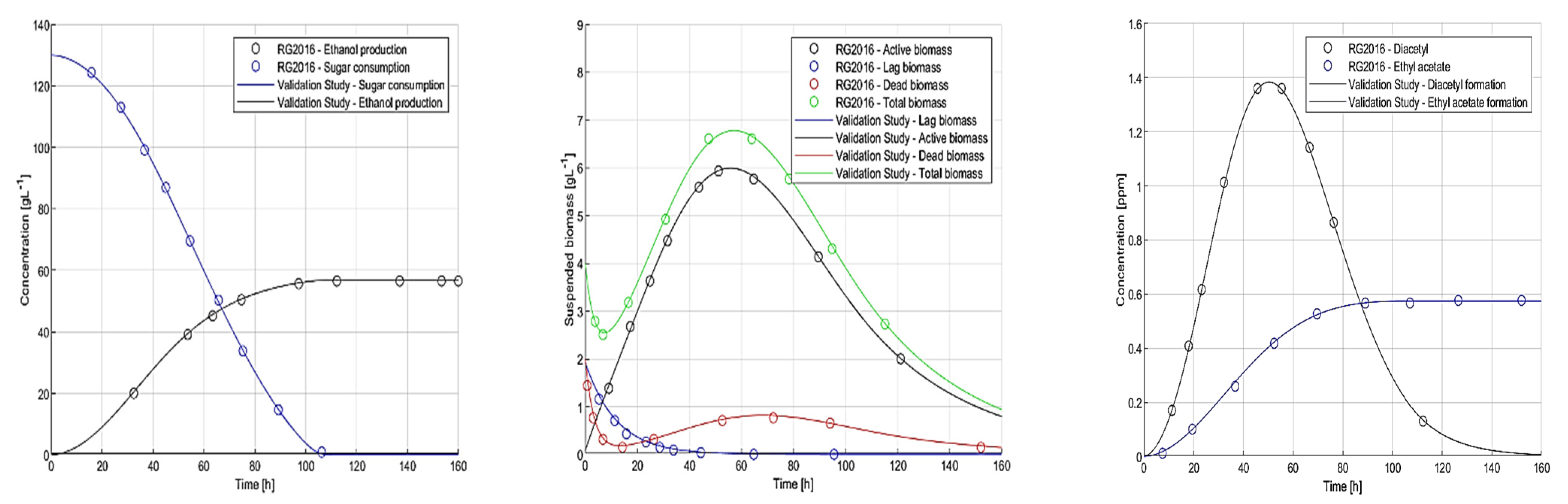
2.4. Dynamic Simulation of Warm Fermentation for Code Validation

To ensure the foregoing mathematical model credibly describes fermentation systems, our script has been used to obtain several responses used for validation after comparison with published results.

The temperature profile for this model validation considers a single isothermal (T = 13 °C) profile incorporated into the model as an interpolation from t₀ = 0 to t_f = 160 h with both initial and final fermentation temperature values at T = 286.15 K. The numerical integration time step employed was Δt = 1 h throughout; we also confirmed that a shorter time step does not improve accuracy.

The temperature profile is critical to the entire model as it governs Arrhenius expressions and therefore determines the magnitudes of each model parameter per unit time, which in turn guides the dynamics of the entire system. At each time node, the parameters are solved for and incorporated into the DAE system, and numerical integration provides results for all response trajectories (Figure 4).

Our simulations yield sugar and ethanol concentration responses throughout this fermentation (T = 13 °C = 286.15 K), for MATLAB code validation purposes vs. our earlier (2016) publication [20].

Figure 4 shows that fermented sugar concentration starts at 130 g L⁻¹, decreasing until completely consumed after 106 h of fermentation, a value coinciding with theoretical (complete) sugar depletion. Ethanol concentration in the fermenter begins at 0 and increases over the duration of the fermentation process until 106 h, after which point no more is produced until the fermentation ends (t = 160 h).

The total suspended biomass is the sum of active, lag, and dead biomass in the fermenter: lag cells decrease from the start until t = 65 h, from when no lag cells are further present in the fermenter. Active cells in the fermenter increase relatively quickly at first, reaching their highest concentration at t = 56 h until they then decrease again throughout the remainder of the fermentation process. Dead cell concentration can be described as dropping precipitously relative to other biomass responses until t = 14 h, before rebounding and increasing until t = 70 h before finally decreasing steadily for the remainder of the fermentation process. The total biomass signal (green line) is the sum of all three responses per unit time and features a minimum (before t = 10 h) and a maximum (about t = 60 h).

Ethyl acetate and diacetyl responses (initial condition: 0 ppm) evolve over fermentation (Figure 4). Diacetyl increases at a high rate, peaking at t = 50 h and tailing off for the rest of the fermentation. Ethyl acetate also increases albeit at a much slower rate, it peaks at t = 106 h (as the ethanol signal) and remains constant thereafter, since sugar (as per concentration signal) is fully consumed at this point.

3. Industrial Processing and Experimental Results

3.1. Process Description

An industrial fermentation for a commercial (0.5% ABV) beer product was performed under CCF conditions, employing an actual batch volume of V = 9.19·10⁴ L in an industrial cylindrical fermenter of volume V = 2.00·10⁵ L (slightly less than half-full) without any use of mechanical stirring. A standard gravity wort was subjected to Saccharomyces pastorianus yeast for this industrial CCF run (wort specifications are provided in

Table 4. Tabulated data from the industrial partner specifying the change in specific gravity (SG), acetaldehyde concentration (ppm) and pH vs. time (fermentation run duration) for a CCF experiment.

Time (h)	Specific Gravity (SG)	Acetaldehyde Concentration (ppm)	pH
0	1.027	0	4.09
12	1.027	(–)	(–)
24	1.026	(–)	(–)
36	1.025	(–)	(–)
48	1.025	(–)	(–)
60	1.024	(–)	4.07
post-dilution	1.015–1.016	24.50	(–)

and Table 6; high-gravity worts have SGs between 1.055 and 1.07). The exact CCF temperature profile was not provided, but varies between T = 5 and 6.5 °C. Three separate temperature profiles were thus inferred as possibilities for investigation; an isothermal at T(t) = 5 °C, another at T(t) = 6.5 °C, and a linear profile increasing from T = 5 to 6.5 °C over a time of t_span = 60 h.

Though other temperature profiles (especially nonlinear) may exist, extending the scope of the problem to probing all putative temperature profiles of interest within the provided industrial range is straightforward to implement if one modifies the bounds for this CCF process (5 °C ≤ T(t) ≤ 6.5 °C).

Following the completion of the said industrial CCF process, the initial batch was diluted using V = 5.55·10⁴ L of water for a total post-dilution volume of V = 1.47·10⁵ L. The final product was then evaluated as per internal procedures, including tasting by an expert flavor panel, along with additional sensory analyses via gas chromatography for the final packaged product (‘final pack’). Details on experimental methods for CCF organic compound determination are provided in [2,5,25,35], with liquid/gas chromatographic methods (HPLC, GC-MS) often used for precision measurements.

The data received were categorized into two sets. The first group consists of responses that are not used in the previously validated de Andrés-Toro et al. model and the second group consists of data for responses used explicitly in the previously validated de Andrés-Toro et al. model (Table 4).

Dashes (–) in Table 4 and

Table 5. Tabulated data specifying change in concentrations of ethyl acetate (C_EA), diacetyl (C_DY), ethanol (C_E), ABV, total suspended biomass (X_S), and sugar (C_S) vs. time (fermentation run duration).

Time (h)	CEA (ppm)	CDY (ppm)	CΕ (g L–1)	ABV (% v/v)	XS (cells·mL−1)	CS (g·L−1)
0	0	0	0	0	3·107	68.1
12	(–)	(–)	(–)	(–)	(–)	(–)
24	(–)	(–)	(–)	(–)	(–)	(–)
36	(–)	(–)	(–)	(–)	(–)	(–)
48	(–)	(–)	(–)	(–)	(–)	(–)
60	5.60	0.032	3.80	0.48	(–)	60.7
Post-dilution	3.50	0.020	2.37	0.30	(–)	38.2–40.8

imply that no concentration data are available for these time points. Industrial data corresponding to alcohol content is usually provided and reported in the literature as units of Alcohol-by-Volume (ABV), defined as the number of cm³ ethanol per 100 cm³ beer or % (v/v). Experimental analysis results which were essential in our study are tabulated in Table 5.

Table 4 and Table 5 indicate that the data provided capture various measured concentrations of interest at the starting point (t = 0), and at either the final and/or the post-dilution value, but not while fermentation evolves (sampling is laborious; offline analyses imply inherent drift and inaccuracy). Offline monitoring of sugars is possible via High Performance Liquid Chromatography (HPLC) [31].

3.2. Flavor Considerations

The composite flavor of beer obtained via CCF is complex, due to the presence of hundreds of flavor compounds [26]. Nevertheless, only total sugar, ethanol, diacetyl, and ethyl acetate were included as responses in the de Andrés-Toro et al. model [41], also employed exclusively in this paper. Thus, it is useful to compare industrial final concentration measurements against established flavor thresholds reported in the literature, to probe the importance of known flavor contributors (

Table 6. Key flavor component concentrations vs. respective thresholds for a 0.5% v/v beer.

Chemical Name	Final Pack Concentration (ppm)	Flavor Threshold (ppm)	Ref.	Flavor Association
Aldehydes (Non-VDK)
2-methylbutanal	4.96·10−3	1.00·10−3	[32]	Almond, apple-like, malty, wort
3-methylbutanal	1.98·10−2	5.60·10−2	[29]	Malty, chocolate, cherry, wort
Furfural	1.12·10−2	1.50·101	[44]	Caramel, bread, cooked meat
Trans-2-nonenal	4.00·10−4	3.00·10−5	[29]	Cardboard, papery, cucumber
Acetaldehyde	2.82·10−3	1.10	[29]	Green apple, fruity
VDKs
Diacetyl	2.00·10−2	1.50·101	[45]	Buttery, butterscotch
Pentane-2,3-dione	1.00·10−2	9.00·101	[45]	Buttery
Fusel alcohols
Propanol	1.70	6.00·102	[46]	Solvent-like
Isobutanol	1.80	1.00·102	[46]	Solvent-like
Esters
Ethyl hexanoate	1.00·10−2	2.00·10−1	[23]	Apple, pineapple
Isoamyl acetate	5.00·10−2	5.00·10−1	[44]	Banana, pear
Ethyl acetate	9.00·10−1	2.10·101	[33]	Fruity, solvent-like

).

Table 6 shows that 2-methylbutanal and trans-2-nonenal were detected at concentrations higher than literature flavor thresholds; this is possibly a manifestation of ‘staling aldehyde’ effects. Surpassing a single flavor threshold does not necessarily have quantifiable sensory implications, given the complex nature of beer, and the possible synergistic or suppressive flavor effects [13,27]. Moreover, the literature flavor thresholds are obtained under controlled conditions (expert panels) and should be judiciously used in regard to pre- and post-dilution points (even more vs. maturation), also noting the fact that different consumer markets generally respond differently to different flavors. Developing a solid understanding of AFB maturation kinetics is critical to such flavor quantification.

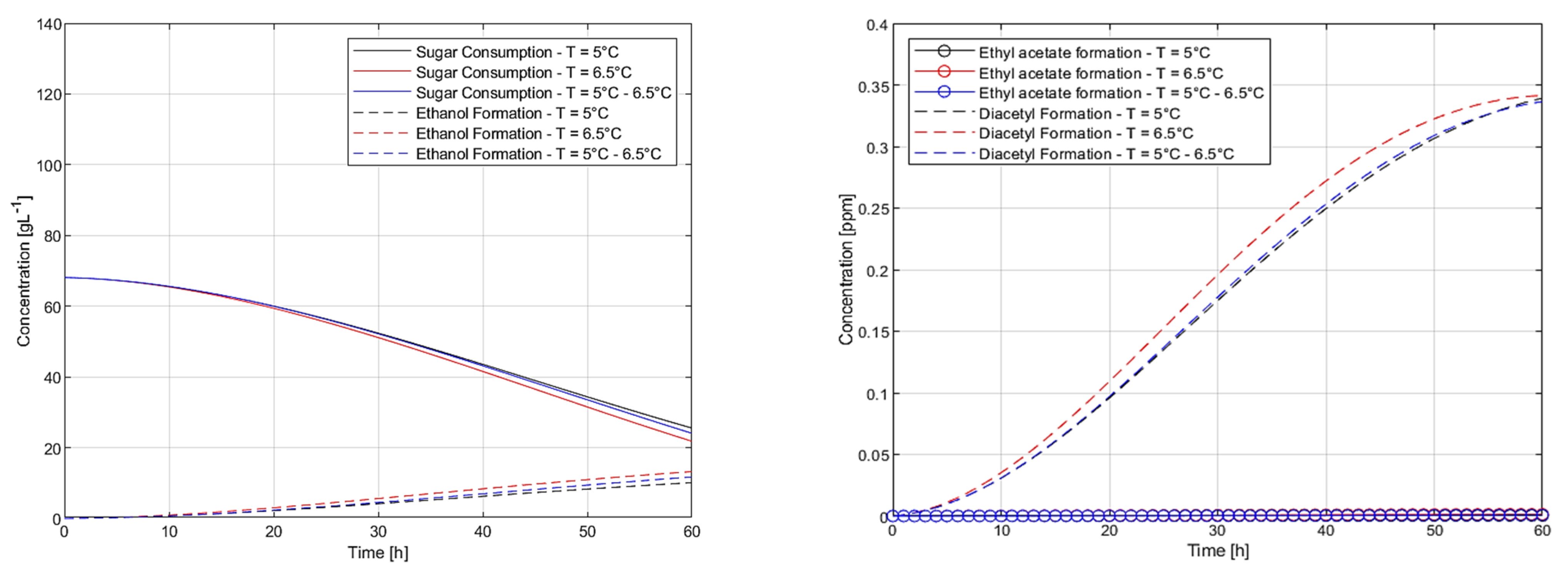
4. Fermentation Response Comparisons

4.1. Initial Condition Considerations

The CCF initial conditions, stipulated temperature manipulation profiles and resulting final concentration measurements are significantly different from warm fermentation results (Section 2.4). To evaluate how the previously validated de Andrés-Toro et al. (Figure 4; T = 13 °C) model functions with different CCF initial conditions (sugar concentration, fermentation duration, and T(t) profiles, as flavor compounds and ethanol are initially zero), several simulations were completed and plotted. Firstly, model response variations for sugar consumption and ethanol formation were assessed (Figure 5).

Even for the lower initial sugar concentration, its complete depletion is not achieved: residual sugar remains after 60 h. Sugar concentration does not match the experimental values reported in Table 5: C_S (60 h) = 20 vs. 60.7 g·L⁻¹. The use of three different temperature profiles produces a relative difference of 5.7% in the values of C_S (60 h) between the lower and higher temperature isotherms. Ethanol production is significantly reduced under these (much colder temperature) conditions, and model results present it as much higher than the final concentration target of C_S (60 h) = 3.7872 g·L⁻¹.

The three different temperature profiles induce a clear relative difference of 15.8% in C_E (60 h) between lower and higher T(t) isotherms, indicating the T(t) profile has a stronger impact on ethanol formation vs. sugar consumption. All these findings imply a clear need for model reparameterization.

Diacetyl and ethyl acetate curves in CCF concentration range (0–0.4 ppm) are provided in Figure 5. Diacetyl formation proceeds faster for the warmest T(t) profile vs. the other two, but the final value variation for C_DY (60 h) is miniscule (0.8%) between the lower and higher temperature isotherms. Ethyl acetate production is extremely limited in all three simulations (C_EA < 1.4·10⁻³ ppm), but for this by-product there is great C_EA(60 h) variation (86%) between the lower and higher T(t) isotherms.

4.2. Comparative Analysis

Current CCF simulations were compared with de Andrés-Toro et al. (T = 13 °C) model results via relative error analysis of state variables (θ). The Relative Percentage Error (RPE) is defined as:

$$\mathit{RPE}=100\left(\frac{{\theta }_{j,\mathrm{IC}}{ - \theta }_{j,\mathrm{dAT}}\left(t\right)}{{\theta }_{j,\mathrm{dAT}}\left(t\right)}\right)$$

(24)

where θ_j,IC denote state variable values (t_span = 60 h) from our init. cond. simulation, and θ_j,dAT(t) is the final state variable value using the de Andrés-Toro et al. (T = 13 °C) model, for t_span = 160 h (Figure 6).

Figure 6a presents RPE results: negative values indicate final-time concentrations smaller than the de Andrés-Toro et al. model results for warm fermentation, with differences being clearly significant.

Figure 6b has a logarithmic RPE scale for comparison of seven state (response) variables with enormous final-time model value differences between the two regimes, which span several orders of magnitude. Only the upper (T = 6.5 °C) and lower (T = 5 °C) temperature profiles are considered (CCF extremes). A higher temperature isotherm generally induces a larger (if not similar) RPE for all concentrations.

Also, C_S has a very high RPE for the higher manipulation, but a much lower one for the lower T(t) manipulation. The remarkable RPE discrepancy for sugar concentration (C_S) is a numerical artifact because of its near-complete consumption at final time in warm (T = 13 °C) but not in CCF (e.g., as seen in Figure 5).

The time horizon considered for dynamic simulations of CCF vs. warm fermentation (Figure 6) is a fair comparison basis in the sense that both processes are complete, but we also note that the span is very different (60 vs. 160 h). Therefore, additional model result comparisons were performed between CCF and warm fermentation initial conditions, this time for all values at t_span = 60 h (Figure 7).

Figure 7a presents RPE results: this time the trend is reversed, with positive values indicating that the time point (and horizon) selected is pivotal (CCF completed, warm run in full swing at t = 60 h). The operational asymmetry (complete vs. mid-time fermentation) is the reason RPE is higher here. Figure 7b has a logarithmic RPE scale to analyze dead cell (X_D) and ethyl acetate (C_EA) concentrations. Lower temperature isotherms produce a slightly larger (positive) RPE for all dynamic state variables, which is the exact reverse trend compared with that of Figure 6 (due to incomplete warm fermentation).

Sugar concentration RPE variations are most pronounced between Figure 6 and Figure 7, but this is hardly surprising due to high (nonzero) initial (C_S) values, and the very low ones upon brewing completion. Ethyl acetate has a very high RPE here (much higher than Figure 6) because its production virtually plateaued as early as t = 60 h at T = 13 °C (Figure 4), but CCF has a much lower final C_EA value (Figure 5).

Model responses to any other T(t) profile between the two isothermal T(t) = 5 and 6.5 °C cases (e.g., the linear upward profile between the two) hence do not need to be comprehensively enumerated. For all T(t) profiles in CCF range, C_EA(t) exhibits conspicuous departure from warm fermentation. Warm fermentation model [41] parameters are thus not reliable for CCF simulation: we note that CCF (low T) seems to suppress undesirable by-product (C_EA) while also reducing alcohol (C_E) generation.

Figure 5 model results grossly underestimate C_EA and overestimate C_E values vs. experiments (Table 5). Though trends are broadly correct, all discrepancies highlight the need for model reparameterization; therein, we only used CCF (without ‘warm’ run) data, to avoid outlier effects and artificial uncertainty.

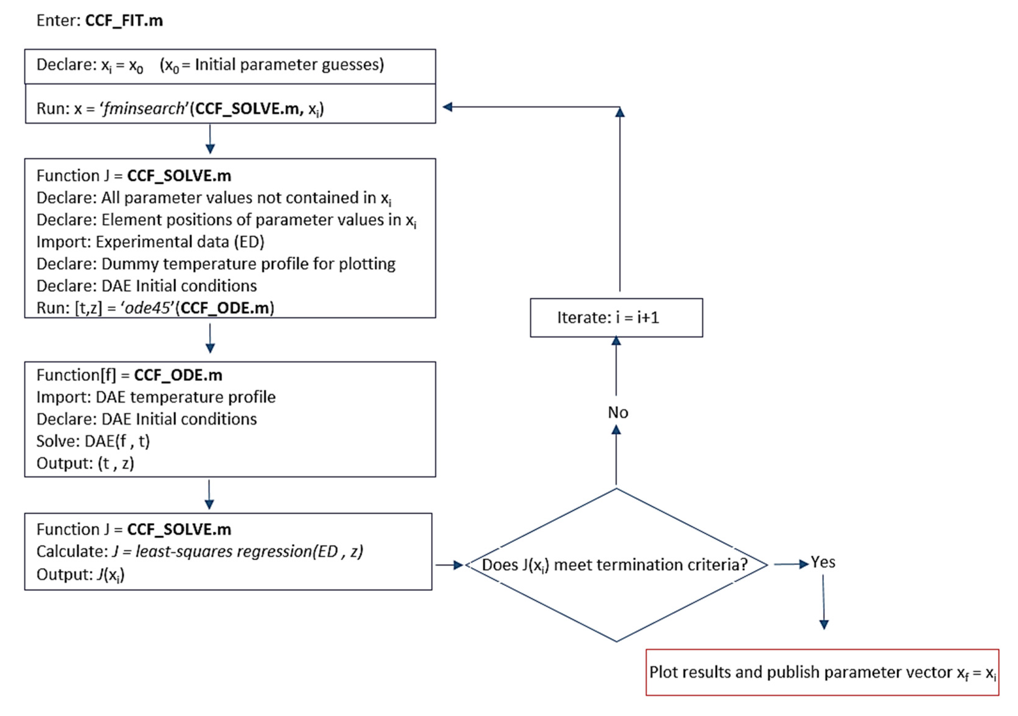
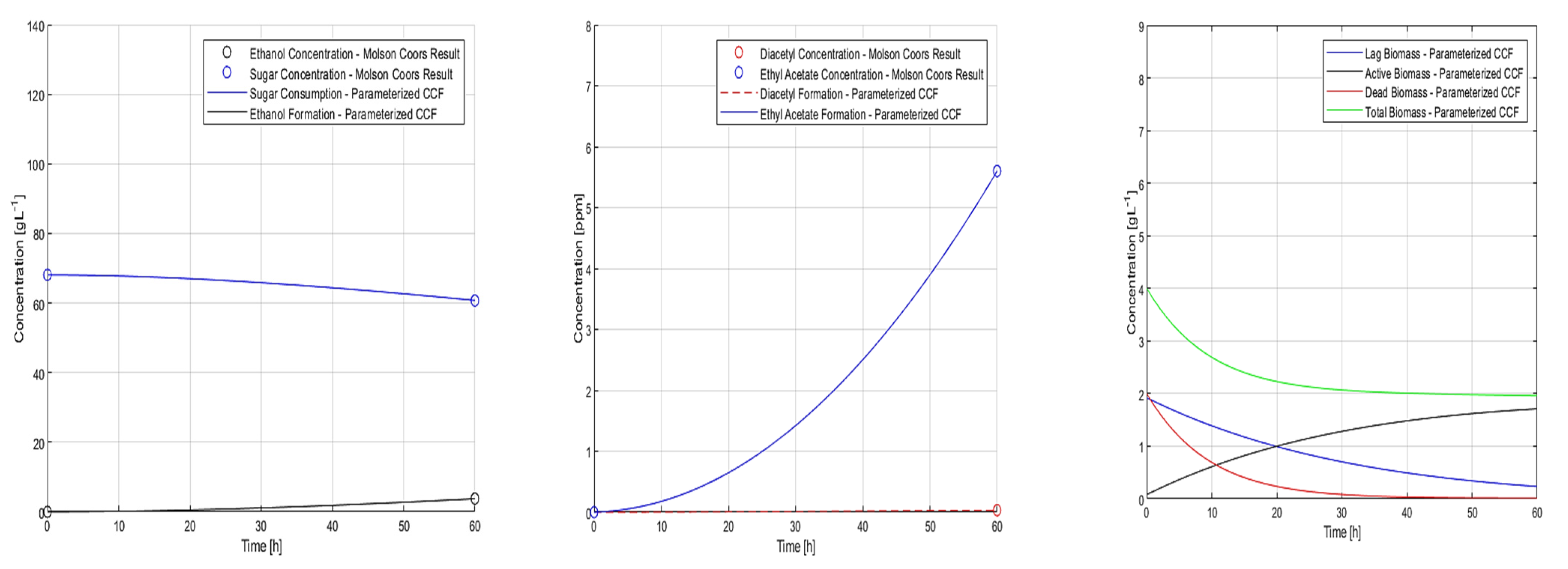
5. Parameter Estimation

5.1. Background

To minimize discrepancies, parameterization of the de Andrés-Toro et al. model for CCF + initial conditions was performed. This parameterization entailed determining a new set of model parameters so that final CCF target responses match experimental data via error minimization:

$$\underset{{\theta }_i}{\min } {J(\theta }_i)$$

(25)

where J is the objective function to be minimized and θ_i is the model response used in minimization. Given the nonlinear dynamic model, an algorithm is required in order to determine a set of parameters (x_f) in a systematic, efficient way. This was performed in MATLAB to minimize the value of least-squares regression between CCF model target responses and experimental data using the Nelder–Mead simplex method (MATLAB’s fminsearch) with tolerances of 1·10⁻⁴ on both decision variables and objective function. An outline of the algorithm and MATLAB code is shown in Figure 8. The Nelder–Mead algorithm is a simplex-based direct search method for nonlinear optimization, minimizing a function of N variables by comparing its values at the N + 1 vertices of a simplex, replacing the highest-value vertex by another point, eventually converging to the minimum [47]. Successive replacements occur via three different operations (reflection, contraction, and expansion).

The least-squares regression (Figure 8) as J is the objective function and formalized generally as:

$$J={\displaystyle \sum }_{i=1}^N{\left({\theta }_{i,\mathrm{measured}}-{\theta }_{i,\mathrm{model}}\right)}^2$$

(26)

The variance-weighted least-squares regression ($J_{\mathrm{VAR}}$) considers a multiplier in the objective:

$${ J}_{\mathrm{VAR}}={\displaystyle \sum }_{i=1}^N\frac{1}{S_{i\theta }^2}{\left({\theta }_{i,\mathrm{measured}}-{\theta }_{i,\mathrm{model}}\right)}^2$$

(27)

where $S_{i\theta }^2$ is the variance according to:

$$S_{i\theta }^2=\frac{1}{N-1}{\displaystyle \sum }_{i=1}^N\left|{\theta }_{i,\mathrm{measured}}-{\overline{\theta }}_{i,\mathrm{measured}}\right|{ }^2$$

(28)

where (N − 1) the degrees of freedom and ${\overline{\theta }}_i$ is arithmetic mean (average). Due to industrial data availability limitations, response variance weighting provided no additional statistical benefit over the standard least-squares regression model (1–2 data points require matching per target response).

A reparameterization solution is achieved by variation in the initial guess vector (x₀) which originally consists of warm fermentation parameter values previously reported in the literature [41]. Convergence requires substantial (>80%) variation in three or more of the target parameter guesses in the correct direction of minimization (e.g., A_YEA, μ_DY, A_μe0), for the reparameterization to be achieved converge within the same number of iterations required by the standard least-squares regression. Non-weighted least-squares regression was used, in the interest of computational efficiency. Weighted least-squares regression may be more advantageous with larger experimental campaigns, due to its power in handling heterogeneous datasets of varying size and possible uncertainty [48,49,50].

5.2. Model Reparameterization Trials

Selecting parameters and numerical values was a key stage of our reparameterization trials. The twelve parameters included in the MATLAB estimation vector (x₀) and varying as unconstrained in the least-squares regression procedure are: A_μe0, B_μe0, B_μS0, A_kes, B_kes, A_μX0, B_μX0, A_YEA, B_YEA, μ_AB, and μ_DY. The six parameters which are not included in the said vector (x₀) are: A_μSD0, B_μSD0, A_μDT, B_μDT, A_μL, and B_μL. A series of trials consider various parameter subsets, to converge to a parameter solution (x₀*) which achieves convergence for the non-fixed components, satisfying initial and final-time data (Table 5).

Beyond Trials 1–2 and the severe non-convergence issues identified, subsequent efforts sought to converge to a credible parameter estimation by first establishing the minimum subset of x₀ components which allow for convergence (Trial 3) and then adding, subtracting, or alternating parameter pairs based on previous trial performance to achieve converging x₀ subsets (Trial 4–8). Once such a parameter vector subset was identified (Trials 9–13), the approach was continued with one-at-a-time changes, to see if and how convergence may be affected by such single substitutions. This approach yields converged solutions without exhaustive enumeration of all possible x₀ subsets, saving CPU expense. Our aim is not the full list of all converged x₀ subsets (these would be prohibitively numerous, because Table 5 data offer very few constraints), but a converged x₀ subset with the minimum norm transition from the original (de Andrés-Toro et al.) parameter values [41].

Table 7. The 17 parameterization trials: parameters computed in each trial (✓) vs. fixed ones (–), and corresponding convergence behavior. ‘Severe’ and ‘slight’ non-convergence indicate problems with multiple or only one response variable vs. final-time industrial data, respectively. Trial 11 yields the final result. The symbol * denotes that (unconstrained) biomass responses exhibit unrealistic behavior.

Trial	Aμe0	Bμe0	AμS0	BμS0	Akes	Bkes	AμX0	BμX0	AYEA	BYEA	μAB	μDY	Result
1	✓	✓	✓	✓	✓	✓	✓	✓	✓	✓	✓	✓	Severe Non-Convergence
2	✓	✓	✓	✓	✓	✓	✓	✓	✓	✓	(–)	✓	Severe Non-Convergence
3	(–)	(–)	(–)	(–)	✓	(–)	✓	(–)	(–)	(–)	(–)	✓	Slight Non-Convergence
4	(–)	(–)	(–)	(–)	✓	(–)	✓	✓	(–)	(–)	(–)	✓	Slight Non-Convergence
5	(–)	(–)	(–)	✓	✓	(–)	✓	(–)	(–)	(–)	(–)	✓	Convergence
6	(–)	✓	(–)	✓	✓	(–)	✓	(–)	(–)	(–)	(–)	✓	Slight Non-Convergence
7	(–)	✓	(–)	✓	✓	(–)	✓	(–)	✓	(–)	✓	(–)	Slight Non-Convergence
8	(–)	✓	(–)	✓	✓	(–)	✓	(–)	(–)	✓	✓	(–)	Slight Non-Convergence
9	(–)	✓	(–)	✓	✓	(–)	(–)	✓	✓	(–)	(–)	✓	Convergence
10	(–)	✓	✓	(–)	(–)	✓	✓	(–)	✓	(–)	(–)	✓	Convergence
11	(–)	✓	(–)	✓	(–)	✓	✓	(–)	✓	(–)	(–)	✓	Convergence
12	✓	(–)	(–)	✓	(–)	✓	✓	(–)	✓	(–)	(–)	✓	Convergence
13	(–)	✓	(–)	✓	(–)	✓	✓	(–)	✓	(–)	✓	✓	Convergence
14	✓	(–)	(–)	✓	(–)	✓	(–)	✓	(–)	✓	✓	✓	Convergence
15	✕	(–)	(–)	✓	(–)	✓	(–)	✓	(–)	✓	(–)	✓	Severe Non-Convergence
16	(–)	✓	✓	(–)	✓	(–)	✓	(–)	✓	(–)	(–)	✓	Severe Non-Convergence
17	(–)	✓	✓	(–)	✓	(–)	✓	(–)	✓	(–)	✓	✓	Convergence

presents the 17 separate cases analyzed, each entailing model parameters computation for each of the three postulated T(t) profiles. A total of 51 trials were conducted with corresponding convergence, iteration, and parameter values recorded. For example, Trial 11 (T = 5–6.5 °C) required 621 iterations and 1029 function evaluations: this is relatively quick compared with several other cases (e.g., Trial 16: 990 iterations; 1586 function evaluations). Trials resulting in slight non-convergence lasted longer than those achieving full convergence; CPU time ranged between 4 min and 2 h.

Trials 1–2 considered most or all twelve parameters to explore the minimization, but failed, indicating too many parameter variations are unsuitable; the opposite approach (starting from fewer unconstrained parameters) bore fruit. Once all trials were completed, the final solution set was determined by computing RPE and performing comparisons in each converging trial pair, and selecting the parameter set that converged via the smallest total parameter (norm) perturbation. This filtering strategy (minimum norm transition heuristic) was conducted since larger parameter differences also induce more drastic departures from the original model parameters published in [41]. Τhe termination tolerance for parameter estimation in our MATLAB optimization code was 1·10^–8, and the final parameter values were obtained by refining the termination criteria to the said value only after RPE yields the best trial (refinement requires 20% longer CPU time; Trial 11: 5.27 min vs. 4.37 min). The RPE values achieved vs. the respective warm fermentation simulations for the same T(t) profile and the parameter values for the Trial 11 set, for each of the three T(t) profiles, are shown in

Table 8. RPE for Trial 11 and corresponding parameter values for the three T(t) profiles (bold: final).

Symbol	CCF (T = 5 °C)	RPE (T = 5 °C)	CCF (T = 6.5 °C)	RPE (T = 6.5 °C)	CCF (T = 5–6.5 °C)	RPE (T = 5–6.5 °C)
μAB	(–)	(–)	(–)	(–)	(–)	(–)
μDY	7.80·10−6	−93.890	7.27·10−6	−94.308	7.59·10−6	−94.054
BYEA	(–)	(–)	(–)	(–)	(–)	(–)
AYEA	123.040	36.832	136.724	52.051	169.130	88.090
Bμe0	(–)	(–)	(–)	(–)	(–)	(–)
Aμe0	2.903	−11.206	4.733	44.744	4.125	26.148
Akes	(–)	(–)	(–)	(–)	(–)	(–)
Bkes	34,658.614	1.329	35,474.587	3.714	35,203.709	2.922
Aμx0	84.280	−22.185	69.395	−35.929	37.450	−65.423
Bμx0	(–)	(–)	(–)	(–)	(–)	(–)
AμS0	(–)	(–)	(–)	(–)	(–)	(–)
BμS0	11,370.511	−2.437	11,950.314	2.536	11,754.776	0.859
AμSD0	(–)	(–)	(–)	(–)	(–)	(–)
BμSD0	(–)	(–)	(–)	(–)	(–)	(–)
AμDT	(–)	(–)	(–)	(–)	(–)	(–)
BμDT	(–)	(–)	(–)	(–)	(–)	(–)
AμL	(–)	(–)	(–)	(–)	(–)	(–)
BμL	(–)	(–)	(–)	(–)	(–)	(–)

.

Table 8 shows a clear (but acceptable) parameter dependence on each T(t) profiles postulated (this is an artifact, as Table 5 offers only a few initial and final points for constraining the estimation). The response curves resulting from the implementation of the new (bold) parameters in Table 8 are plotted to confirm that the newly parameterized CCF model system replicates the industrial results, using the linearly increasing temperature profile, T = 5–6.5 °C over the batch duration of t_span = 60 h. Figure 9 presents the dynamic state responses for this nonisothermal T(t) profile, which is plausible due to exothermic fermentation reactions; the biomass activation is gradual and much slower vs. Figure 4.

Sugar, ethanol, ethyl acetate, and diacetyl responses were plotted to analyze CCF (Figure 9). Reparameterized model responses of sugar and ethanol concentration match both the initial and final industrial data points. The smooth shape of both curves features a slow decrease rate for sugar consumption and a slow increase rate for ethanol formation, over the entire course of fermentation. Biomass fraction responses are also plotted (Figure 9); because industrial biomass data are not provided, the respective biomass curves are unconstrained functions in our foregoing reparameterization. Diacetyl concentrations are about two orders of magnitude smaller than warm fermentation values, while diacetyl dynamics are simpler (monotonic) due to very slow evolution, in contrast to Figure 4. Ethyl acetate concentration, though, is clearly higher (by about an order of magnitude) compared with the final-time warm fermentation values, as already evident by comparing Figure 4 vs. Table 5 values.

Table 9. Warm fermentation parameters of de Andrés-Toro et al. [41] and new CCF values (bold: this study).

Rates and Factors	Description	Ai	Bi
μSD0	Maximum dead cell settling rate	33.820	−10,033.280
μx0	Maximum cell growth rate	37.450	−31,934.090
μS0	Maximum sugar consumption rate	−41.920	11,754.776
μe0	Maximum ethanol production rate	4.125	−1267.240
μDT	Specific cell death rate	130.160	−38,313.000
μL	Specific cell activation rate	30.720	−9501.540
ke = kS	Affinity constant for sugar and ethanol	−119.630	35,203.709
YEA	Stoichiometric factor, ethyl acetate production	169.130	−26,589.000
μDY	Rate of diacetyl production	7.590·10−6
μAB	Rate of diacetyl consumption	1.138·10−3

summarizes the full parameter set for the reparameterized CCF model (including those that were chosen to remain unchanged), as well as diacetyl formation and consumption rates. Boldface denotes new CCF parameter values; the rest remain as per de Andrés-Toro et al. model [41]. The new CCF parameter values only best correspond to the specific T(t) profile and shift for others, as evident in Table 8 (any slight profile variation, even for either isothermal, yields different values). This is not only due to the given uncertainty in the industrial run from which Table 5 data emerged, but also due to the limited (loose) constraining of the CCF model, and the lack of mid-point C(t) data.

5.3. Summary

The MATLAB parameter estimation code we developed employs the Nelder–Mead direct search algorithm to reparameterize the de Andrés-Toro et al. model [41] to describe CCF process conditions. Performance strongly depends on initial guess vector (x₀) and understanding of change directions for each parameter, to successively add/removex₀ components and arrive at a converged solution set x_f. The standard least-squares regression objective was used for al CCF parameterization trials, and the various converged solutions (x_f) were filtered via RPE to obtain the best parameter vector, i.e., that with the shortest deviation vs. the warm fermentation case, for the most realistic CCF T(t) profile. The complete CCF parameterized model is thus provided by Equations (5)–(23), with data from Table 8 and Table 9.

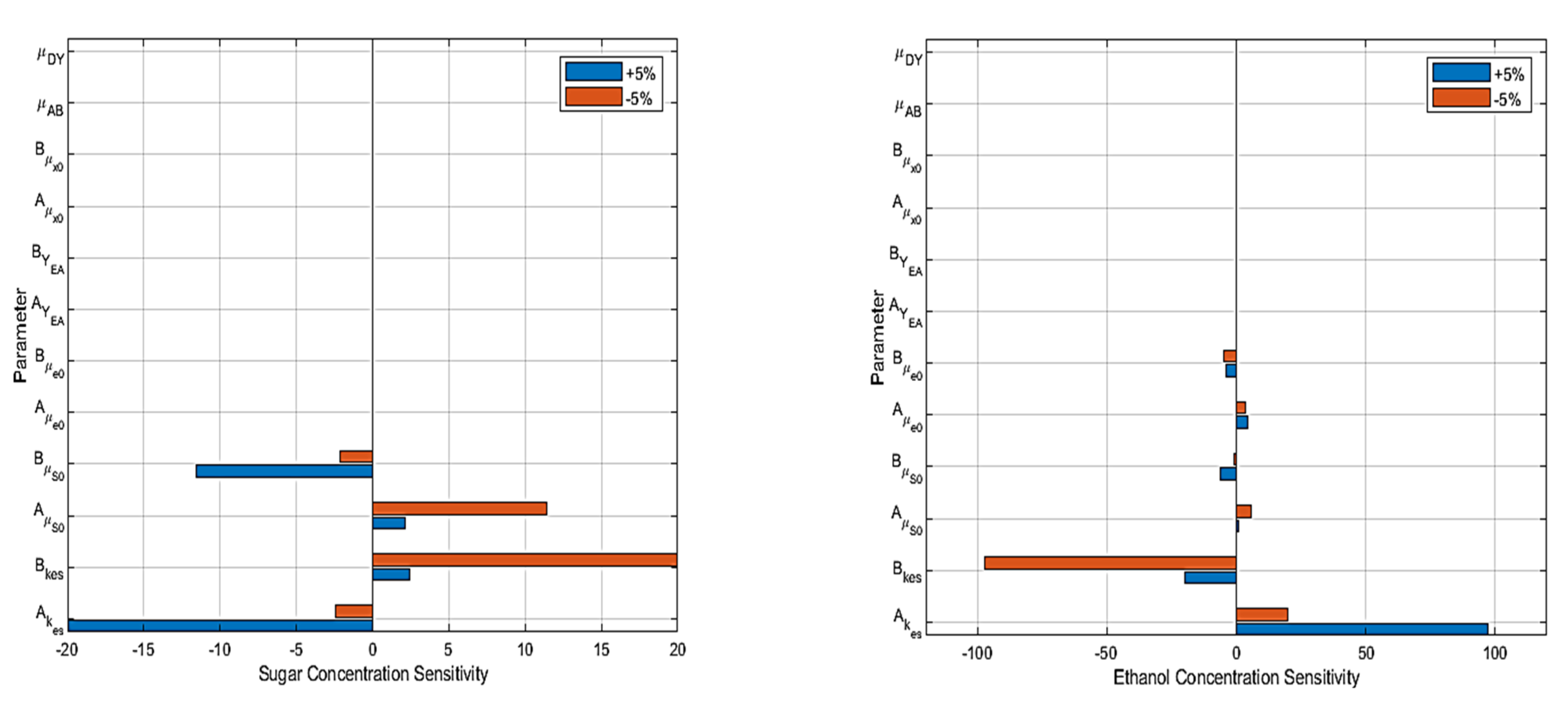
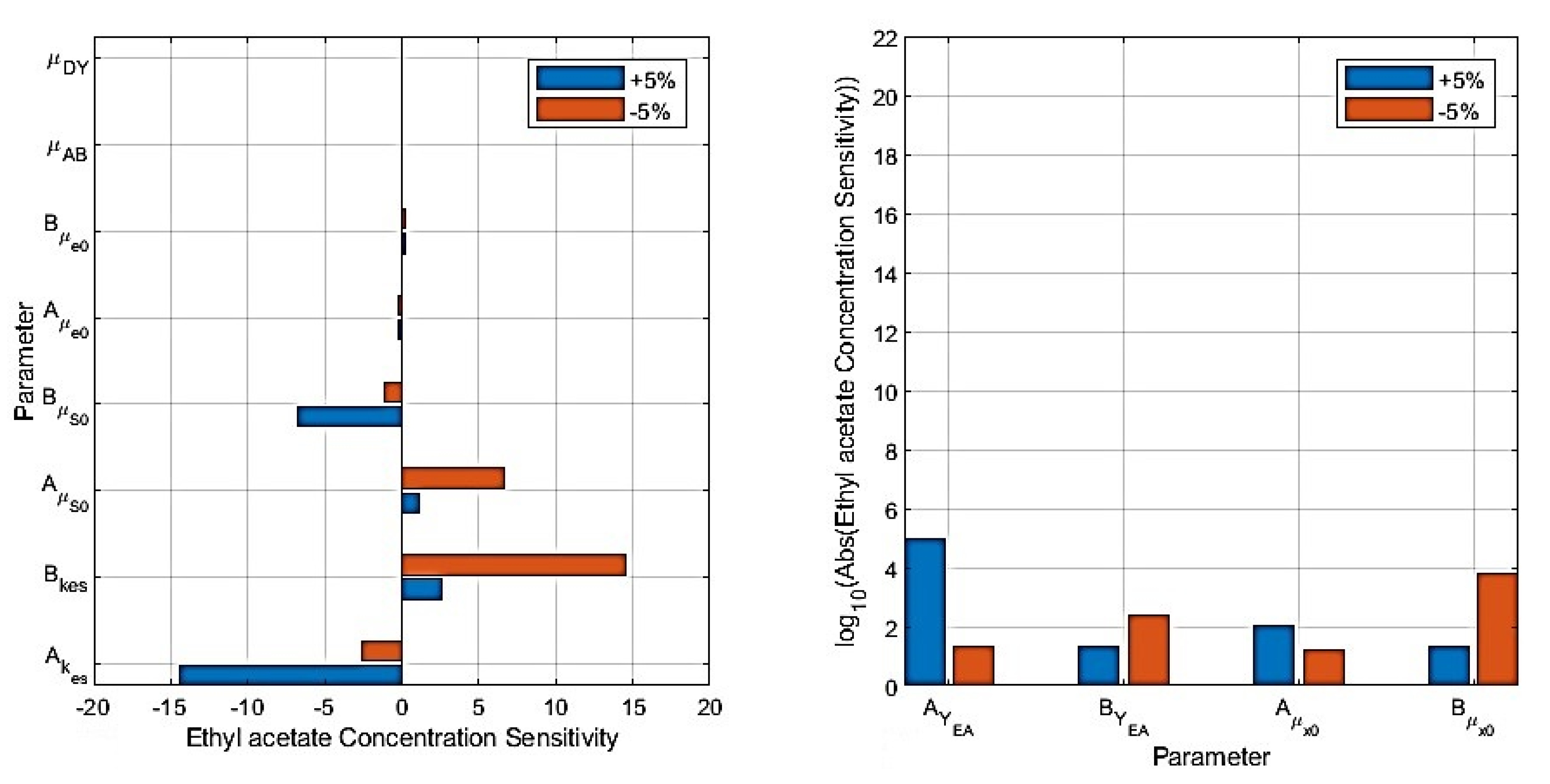
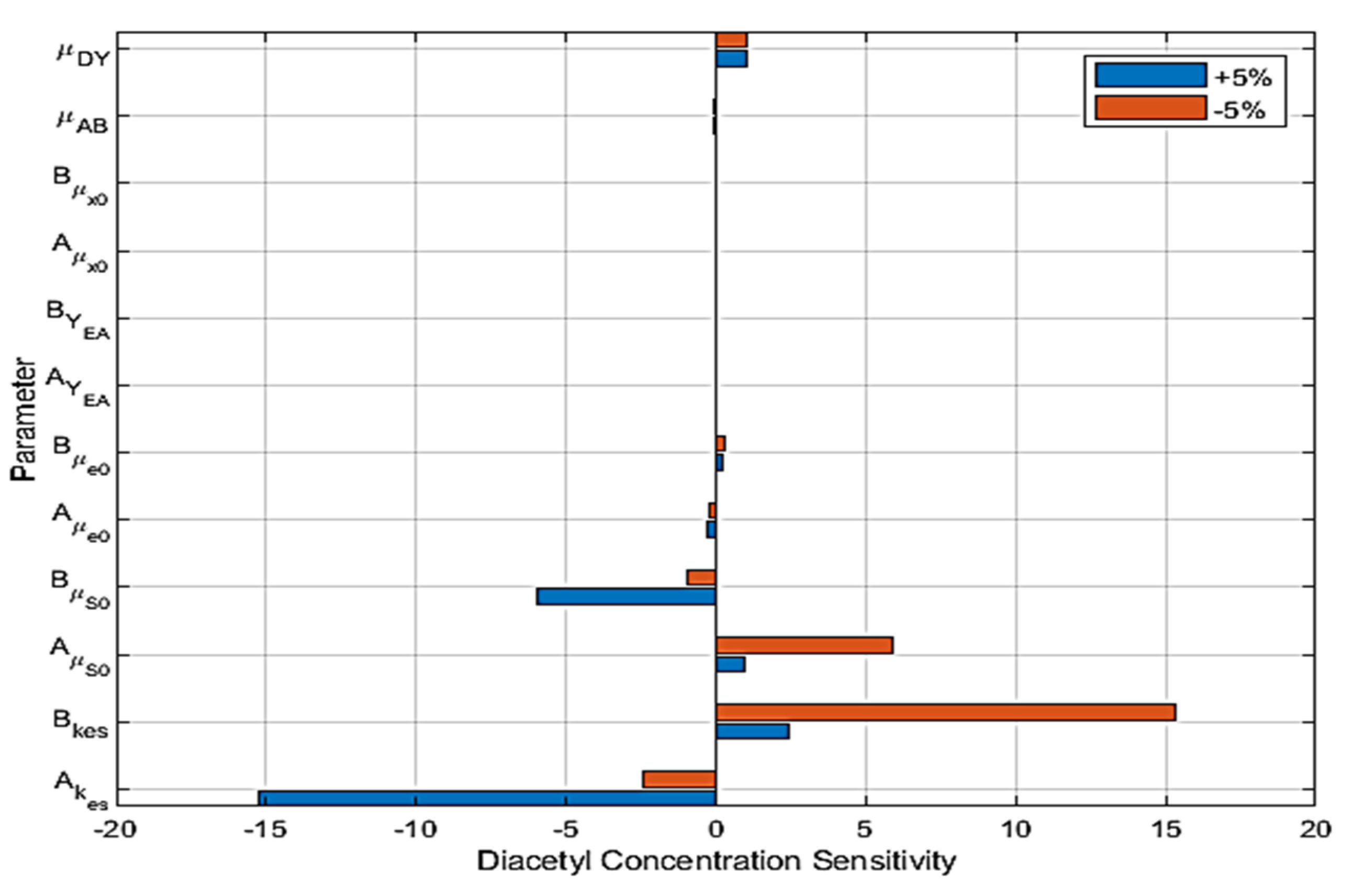
6. Sensitivity Analysis

Sensitivity analyses are performed on dynamic models for a given set of operating conditions, with respect to changes in target model parameters. They provide further understanding of dynamic system responses and are essential prior to optimization [24]. This extra level of model understanding is critical for batch and semi-batch operations that can exhibit very low sensitivity to control policies. Sensitivity S quantifies state variable variation with respect to model parameter changes [47,48,49,50], as:

$$S=\left[\left(\frac{\partial \theta }{\theta }\right)/\left(\frac{\partial P}{P}\right)\right]$$

(29)

where θ denotes the vector of dynamic states of interest, P is the parameter vector that varies, and $\partial \theta$, $\partial P$ are the corresponding state and parameter changes (finite differences), respectively. Large sensitivities provide insight, implying parameters whose uncertain (inaccurate) estimation can induce enormous model vs. process output deviations, hence must be carefully assessed for control. Low sensitivities, accordingly, imply that parameter estimation errors have limited operational effect.

Sensitivity analyses are local or global: the former consider small parameter perturbations, while the latter explore effects of large and/or simultaneous parameter changes on model fidelity [48,49,50]. We focus here on local sensitivity analyses performed for ±5% and ±25% parameter variation for each of the set of 12 potentially crucial parameters (variation above 25% induces severe non-convergence issues within DAE). Variations in 5% are sufficiently small to show sensitivity differences between different model parameters, maintaining relevance to our RPE values from parameterization trials.

Final key compound concentration sensitivities are computed and are illustrated in Figure 10, Figure 11 and Figure 12.

Sugar concentration (C_S) is most sensitive to changes in the parameters A_kes and B_kes, followed by the effects of variations in A_μS0 and B_μS0. Though the effect of parameter variation on final sugar concentration appears to be inverted for parameter pairs, this is not always the case, as shown in succeeding sensitivity analyses. Actual values for all remaining pairs are on the order of 1·10⁻⁹–1·10⁻⁸ (very close to solver tolerance, 1·10⁻⁹), rendering final sugar concentration sensitivity insignificant.

Final ethanol concentration (C_E) sensitivity to ±5% parameter changes is illustrated in Figure 10. Here, as for C_S, A_kes and B_kes variations again produce the largest final ethanol concentration changes. The sensitivity of final ethanol concentration is roughly five times larger (for A_kes and B_kes variation) than the sensitivity of final sugar concentration to identical A_kes and B_kes changes, but of opposite sign. Variations in A_μS0, B_μS0, A_μe0, and B_μe0 produce similarly sized changes in final ethanol concentration. All other sensitivity values for other target parameters are in the order of 1·10⁻⁸, hence insignificant.

Final ethyl acetate concentration (C_EA) sensitivity to ±5% parameter changes is shown in Figure 11: therein, A_YEA and B_μx0 emerge as most influential on ethyl acetate concentration, followed by B_YEA and then A_μx0 and all remaining parameters depicted. Sensitivity values for μ_AB and μ_DY are on the order of 1·10⁻⁸–1·10⁻⁷, and for the foregoing reasons, insignificant vs. final ethyl acetate (C_EA) concentrations.

Final diacetyl concentration (C_DY) sensitivity to ±5% parameter changes is presented in Figure 12: A_kes and B_kes have the strongest impact, followed by A_μS0, B_μS0, and μ_DY. The two parameters directly related to diacetyl formation and consumption (μ_DY and μ_AB) do not induce the largest sensitivity (other parameter sensitivities are of the order of 10⁻⁶, their effect hence being insignificant).

Final ethyl acetate concentration is by far the most sensitive to parameter variation, followed by ethanol, sugar, and diacetyl responses; C_EA sensitivity is highest for A_YEA changes, while all other state variables respond strongest to A_kes and B_kes variations. Clearly, small CCF initial condition and/or T(t) changes may induce key model response drifts, implying critical process (product quality) variation. The high sensitivity of many responses to A_kes and B_kes changes is justified by recognizing that they directly affect sugar consumption and ethanol formation, and indirectly (through ethanol) diacetyl levels. Sugar concentration is critical [51]: it governs biomass proliferation which drives ethanol, diacetyl, and esters formation. Thus, all parameters affecting C_S and C_E induce composite (synergistic) effects. Conversely, A_μx0 and B_μx0 variation generally induce minimal response change (excluding C_EA levels).

7. Coarse Grid Enumeration of Plausible Temperature Manipulation Profiles

A conceptual CCF process may operate in a tight (1.5 °C) temperature band (T = 5–6.5 °C), although it is recognized that CCF can be performed for T = 0–8 °C [8,14,16,17,18,19,20]. The use of cooling jackets allows for implementing industrial fermentation T(t) profiles with temperature changes, provided that the fermentor is not cooled excessively and that enough reaction heat is produced [20]. Our goal is to gain insight into responses computed from our CCF model parameterization for different plausible T(t) profiles, beyond isothermal or tightly restricted ‘constant and increasing’ ones.

Quantifying the effects of imposed T(t) profile variability on final-time beer quality is achieved via monitoring the respective vector of concentrations, [C_S(t = t_f), C_E(t = t_f), C_EA(t = t_f), C_DY(t = t_f)]^T. Multiobjective process optimization for brewing intensification at lower cost with flavor consistency has been the focus of many studies on warm (but few on cold) fermentation over three decades [20,21,22,23,24,30,31,32,33,34,35,36,37,38,39,40,41,42,43,44]. To comprehensively explore operational options in a wide temperature range, we can construct a set of feasible T(t) manipulation profiles and evaluate the resulting final-time concentration vectors [20].

To enumerate plausible T(t) manipulation profiles, the CCF time domain (60 h) is discretized into an initial ‘coarse grid’ (6 intervals; 10 h each). The temperature domain is discretized in six 1 °C intervals, from T = 1 °C up to and including T = 7 °C, yielding a 36-block canvas of 49 nodes (Figure 13). This larger, more inclusive T(t) span is selected based on the theoretical range (0–8 °C) reported in the literature [8,14,16,17,18,19,20], and is constrained because operating at T < 1 °C outside of a laboratory is unrealistic (too close to water freezing is very problematic for industrial operations and instruments). Temperatures T > 7 °C are omitted for the reasons underlying the de Andrés-Toro et al. model [41]. Finer time grids are possible (at extra CPU expense), but finer T(t) grids are pointless vs. sensing.

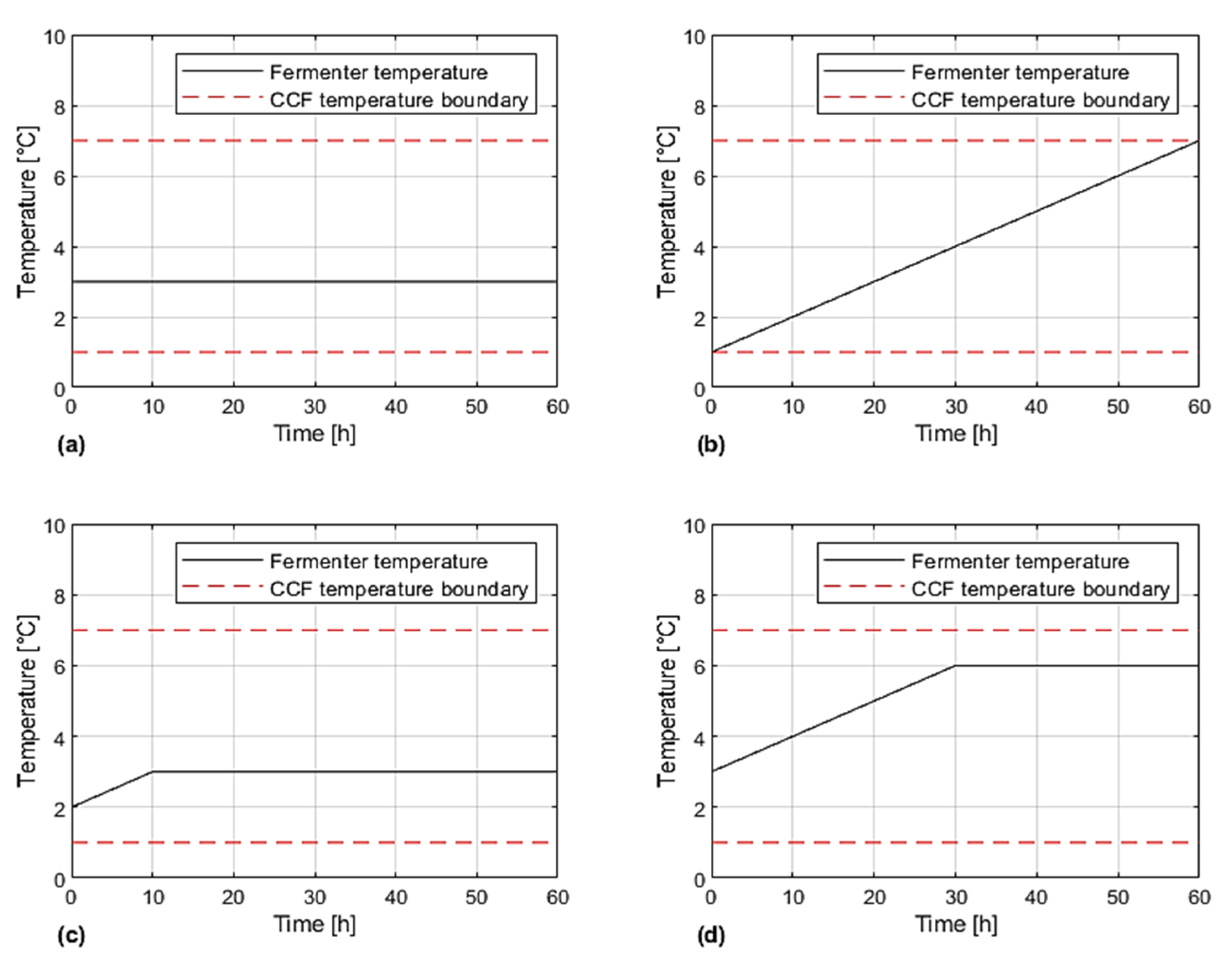
7.1. Heuristics for Plausible Temperature Manipulation Profiles

To perform enumeration, we use a set of heuristics to limit the ensemble of plausible T(t) profiles. The rationalizations for many of them emerge conceptually from published cost functions for beer fermentation control optimization via deterministic or stochastic (genetic) algorithms [20,21,22,41,42,43]. This happens for two reasons: to ensure T(t) profiles correspond to feasible industrial manipulations, but also to achieve a tractable total number of plausible T(t) profiles within reasonable CPU expense.

Heuristic 1: Temperature profiles can be isothermal along the entire computational domain.

Reasoning: Fermentations may progress with T changes smaller than detectable instrum. limits (1 °C).

Heuristic 2: Temperature profiles can monotonically increase in the entire fermentation time domain.

Reasoning: Fermentations may result in increasing batch temperatures throughout the CCF process.

Heuristic 3: The CCF process may begin and end at any temperature between T = 1 and 7 °C.

Reasoning: The said temperature range for CCF operation is established in the literature [1,2,3,9].

Heuristic 4: The temperature difference between successive time nodes may not exceed 1 °C.

Reasoning: Implemented to reflect operability vs. curse of dimensionality (fewer plausible T profiles).

Heuristic 5: Any number of isothermal segments (10 h) can succeed any number of increasing T ones.

Reasoning: Fermentations may progress as a mix of isothermal and exothermic segments in the vessel.

Heuristic 6: A time period of increasing temperature cannot succeed a period of isothermal activity.

Reasoning: The fermentation process is continuous and assumed here to exclude effects of hysteresis.

Heuristic 7: The temperature in the fermenter cannot decrease at any point.

Reasoning: Excessive CCF cooling obstructs biochemical activity, effectively delaying fermentation.

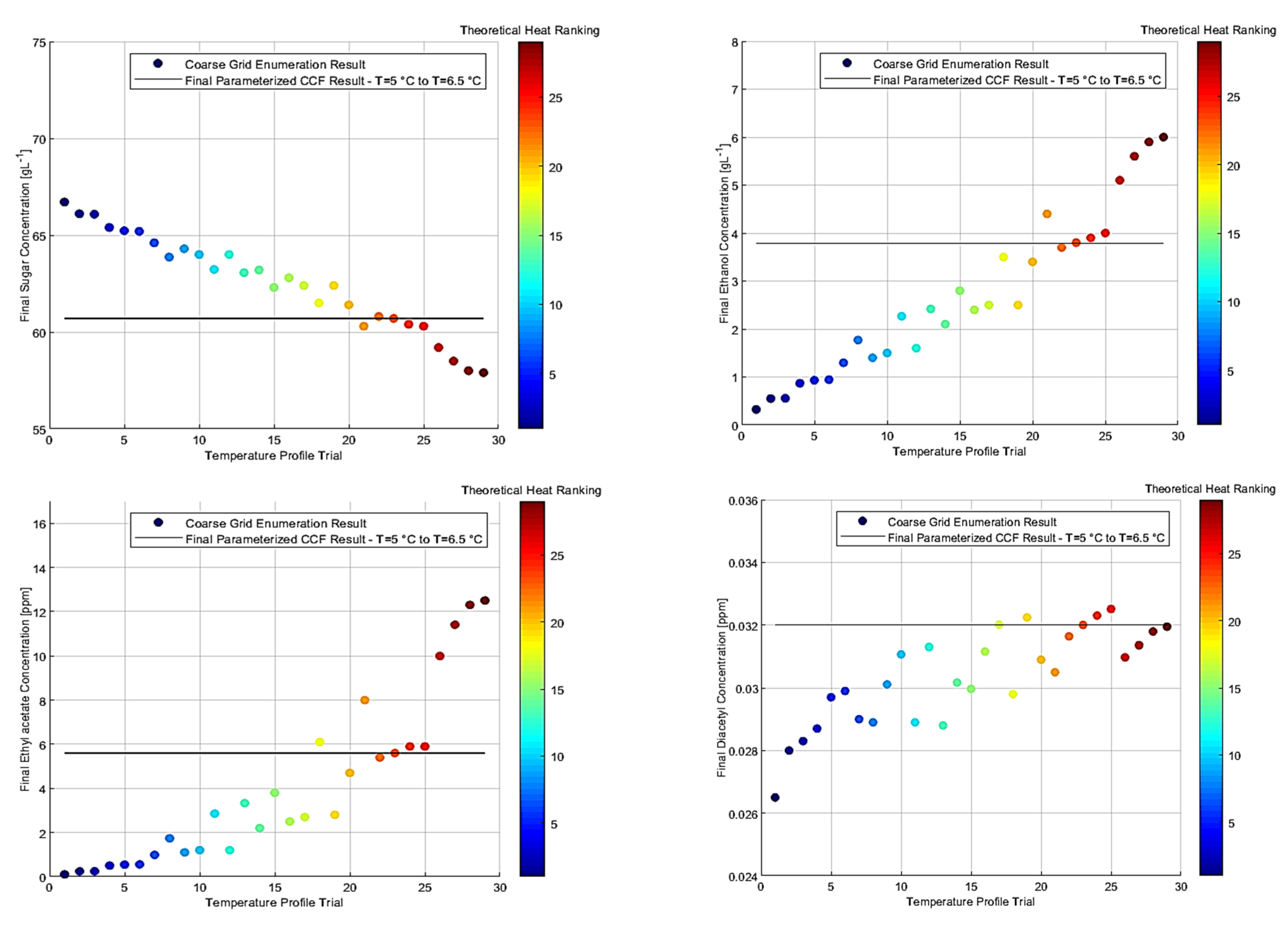
7.2. Effect of Total Theoretical Heat Input on Final-Time CCF Concentrations

The said heuristics enable the classification of plausible T(t) manipulation profiles in four groups (Figure 13): temperature profiles used, corresponding trial numbers, and types, are detailed in

Table 10. Candidate CCF temperature manipulation profiles (°C) ranked vs. Q (Trial 23: threshold).

T(t) Trial	T(t = 0)	T(t = 10)	T(t = 20)	T(t = 30)	T(t = 40)	T(t = 50)	T(t = 60)	Type
1	1	1	1	1	1	1	1	a
2	1	2	2	2	2	2	2	c
3	2	2	2	2	2	2	2	a
4	1	2	3	3	3	3	3	d
5	2	3	3	3	3	3	3	c
6	3	3	3	3	3	3	3	a
7	1	2	3	4	4	4	4	d
8	1	2	3	4	5	5	5	d
9	2	3	4	4	4	4	4	d
10	3	4	4	4	4	4	4	c
11	1	2	3	4	5	6	6	d
12	4	4	4	4	4	4	4	a
13	1	2	3	4	5	6	7	b
14	2	3	4	5	5	5	5	d
15	2	3	4	5	6	6	6	d
16	3	4	5	5	5	5	5	d
17	4	5	5	5	5	5	5	c
18	2	3	4	5	6	7	7	d
19	5	5	5	5	5	5	5	a
20	3	4	5	6	6	6	6	d
21	3	4	5	6	7	7	7	d
22	4	5	6	6	6	6	6	d
23	5	5.25	5.5	5.75	6	6.25	6.5	(–)
24	5	6	6	6	6	6	6	c
25	6	6	6	6	6	6	6	a
26	4	5	6	7	7	7	7	d
27	5	6	7	7	7	7	7	d
28	6	7	7	7	7	7	7	c
29	7	7	7	7	7	7	7	a

. Trials are classified by total theoretical heat input (Q), from lowest (Trial 1) to highest (Trial 29) value.

The total theoretical heat input (Q) provided to the CCF fermentor mixture (ignoring losses) is:

$${ \mathrm{Q}=\mathrm{mC}}_{\mathrm{p}}\underset{{\mathrm{t}}_0}{\overset{{\mathrm{t}}_{\mathrm{f}}}{{\displaystyle \int }}}\mathrm{T}\left(\mathrm{t}\right) \mathrm{d}t$$

(30)

where Q is the theoretical heat input, m is the fermentation mass, C_P is the specific heat capacity of the mixture, T(t) is the fermentor temperature and time dt spans the fermentation interval t = 0–60 h. This definition is operationally equivalent to the total theoretical enthalpy of the mixture at any time, as T(t) is the net effect of exothermic CCF reactions and heat removal from the system (cooling jacket). Actual industrial fermentor heat transfer dynamics are a lot more complex, but easy to address [23]. Specific Q values are not provided, as they are only used for ranking and plotting final concentrations (Figure 14).

Final sugar concentration (C_S) ranges between 57.9 and 66.7 g·L⁻¹ for the T(t) profiles of Table 10, implying higher heat input (Q) induces greater sugar consumption up to Trial 8 and after Trial 21; the respective segments (Trials 1–8, 21–26) appear monotonic, whereas Trials 9–20 show oscillations.

Final ethanol concentration (C_E) ranges between 0.3 and 6.0 g·L⁻¹ for the same temperature profiles, (a 20-fold span depending on T(t) variation), also increasing as a function of theoretical heat input Q. Trials 8–26 again show oscillation in between linear trends; this is key for CCF ethanol minimization.

Another important conclusion is drawn by observing the right end of all four panels of Figure 14. Response grouping for Trials 22–25 and 26–29, indicate two sets of CCF processes which are very similar in terms of total theoretical heat input (thus resulting in very similar expression of ethanol), but also very different in terms of flavor compound (diacetyls, esters) expressions in the final product. A distinct jump is remarkable between Trials 25 and 26; in the latter, a high T = 7 °C is used for 40 h. This clearly implies a hard thermal threshold which must be avoided during industrial CCF runs, given the definitive requirement for low final ethanol (perhaps also low total ester) concentrations.

Final ethyl acetate concentration (C_EA) ranges between 0.1 and 12.5 ppm for the temperature profiles, and it is generally (not always, e.g., Trials 8–19) increasing as a function of theoretical heat input (Q). Trials 1–8 have a linear trend, before the oscillatory behavior. A 70% jump between Trials 25 and 26 (using T = 7 °C for 40 h or longer), implies a threshold to be avoided, to prevent a high-Q C_EA surge. Figure 14 shows a potentially useful high C_EA sensitivity to small temperature changes: a small heat input change can strongly impact ester expression (Trials 25–26) without comparable changes in other flavor compounds, esp. as esters are typically near or just above beer flavor threshold values [20,21,22,23,24]. Minor process changes can induce beneficial flavor variations, as esters boost fruitiness (cf. Table 6).

Final diacetyl concentration (C_DY) ranges between 2.6 and 3.2·10⁻² ppm for these temperature profiles and remains in all cases (Trials 1–29) within specifications (26–32 ppb) (cf. different C_EA vs. C_DY scales). Final C_DY generally rises with T(t) profiles of higher Q, with pronounced oscillations after Trial 6. Flavor thresholds for C_EA and C_DY are of the same order of magnitude, so our reparameterized model implies there is great potential for beneficial ester (vs. diacetyl) expression under CCF conditions [33].

A set of four different temperature profile types (based on seven constraint heuristics) were used for CCF model response enumeration, in the acceptable temperature range of 1–7 °C. Employing a coarse time grid discretization, dynamic simulations were ranked by total theoretical heat input (Q) received by the fermentation system, yielding a series of colormaps illustrating temperature profile variation effects on key final observable (sugar, ethanol, diacetyl, and ethyl acetate) concentrations.

Simulations for higher theoretical heat (Q) show higher sugar consumption and higher ethanol, ethyl acetate, and diacetyl production for warm brewing [20,21,22,23,24]. Temperature profiles of T = 7 °C for 40 h or more yield a surge in ethanol and ethyl acetate production, and high sugar consumption. Diacetyl expression varies much less (within 6 ppb), implying ethanol and ethyl acetate sensitivities are of much greater concern. Identical theoretical heat (Q) inputs may have very different effects, depending on the CCF T(t) profile chosen. Though a concern from a process control perspective, this may enable small but extremely beneficial to flavor changes without any major process modifications.

8. Conclusions

CCF is one of the best LAB/AFB brewing methods due to simplicity, cost-effectiveness, and limited alterations required to fermentation step temperature profile and duration. Modern industrial implementation attests to its efficiency vs. other methods developed over the last few decades [3,9]. Concerns regarding flavor remain: this paper aims to not only explore T(t) effects and response outputs between warm fermentation and CCF, but also to construct a reparameterized model which accurately describes the physical CCF process with regard to hypothetical changes and sensitivities.

The de Andrés-Toro et al. first-principles model [41] was used due to its predictive fidelity and the concise number of data points available for validation. The MATLAB (DAE) code constructed matches and published model simulations for T = 13 °C, and was used for quantitative comparisons between warm fermentation and CCF model responses. A CCF model reparameterization via industrial data (initial and final sugar, ethanol, diacetyl, and ethyl acetate values) and sensitivity analysis followed. Finally, a ‘coarse grid enumeration’ was performed to analyze the effect of plausible T(t) profiles on CCF brewing, showing reduced ethanol production generally coincides with lower flavor expression.

Model reparameterization is instrumental, as per RPE comparisons between model responses for CCF vs. de Andrés-Toro et al. (T = 13 °C) process conditions: CPU expense is relatively small but varies widely with trial conditions. Convergence and speed depend on parameter subset selection. The Nelder–Mead algorithm with least-squares regression performed well in this study, yielding parameter values which achieved full CCF model matching against the concise industrial dataset used. New CCF parameters are not vastly departed from warm brewing [20,21,22,23,24,41], with RPE within an order of magnitude; future efforts must use larger datasets and global optimization algorithms [49].

A sensitivity analysis indicates that parameters A_kes and B_kes are the strongest influencers of response variation, due to the great importance of sugar, ethanol, and biomass in model dynamics. Ethyl acetate is the most sensitive response vs. parameter variations, confirming that ester expression is an indispensable LAB/AFB process control target, given its dominance on fruitiness perception.

Coarse grid enumeration reveals a global increase trend for sugar consumption and ethanol, ethyl acetate, and diacetyl formation with increasing theoretical heat input (Q). Ethanol and especially ethyl acetate formation are most sensitive to T(t) profile variation, with output variation ranges much larger than sugar consumption and diacetyl formation. Results clustering show that small T(t) profile changes can greatly benefit product flavor and quality. A trade-off is clear, as CCF aims for ethanol reduction without flavor loss, but targets all rise together, yet at different rates. Experiments for flavor improvement may result in higher ethanol expression, but post-process dilution compromises flavor. Product refinement must focus on relative flavor compound change rates within narrow temperature intervals, possibly smaller batches, and external preheating/cooling/agitation for best process control.

The development of select T(t) profiles indicates that not all are necessarily possible without heat exchange (cooling) during CCF. For any given hypothetical T(t) profile with a confirmed promise of improved results over current CCF, extra capital expenditure is needed that may offset AFB profits, as fermenters typically comprise only cooling jackets. When the resulting AFB product is of superior flavor and quality (confirmed via simulations and pilot plant experiments), the benefit is warranted.

Multiobjective CCF optimization requires much larger datasets (more measured inputs/outputs, higher data density), as biomass responses here (and CCF mid-time points) are left unconstrained. Performing ‘what if’ analyses (e.g., enumeration) requires more extensive CCF model validation to accurately predict T(t) profile variation effects within tight ranges. No consideration of yeast strain effects, initial sugar/biomass concentration, and fermentation duration is considered here (all are assumed constant due to industrial conditions). The best process in terms of flavor, quality, and processing time can emerge from a combined approach, using additional processing steps and/or treatment methods (pre-/post-processing), after evaluating the impact of manipulations on efficiency.

Though the de Andrés-Toro et al. model is powerful via its reduced number of state variables, additional flavor compounds must be considered to better capture more beer flavor dimensions. Dynamic models cannot easily capture bitterness or wortiness (due to carbonyls of e.g., acetaldehyde and 2-/3-methylbutanal), both compromising LAB/AFB flavor; however, more model compounds increase DOF and require larger datasets to ensure and maintain high model fidelity. Potential new parameterizations towards CCF intensification thus require data acquired over a finer time domain discretization, with more flavor coordinates and fewer temperature profile heuristics.

References

1. Southby, E.R. A Systematic Handbook of Practical Brewing; Franklin Classics: Oxford, UK, 1885. [Google Scholar]
2. Boulton, C.; Quain, D. Brewing Yeast and Fermentation; Elsevier: Amsterdam, The Netherlands, 2001. [Google Scholar]
3. Liguori, L.; Russo, P.; Albanese, D.; Di Matteo, M. Production of low-alcohol beverages: Current status and perspectives. In Food Processing for Increased Quality and Consumption; Elsevier: Amsterdam, The Netherlands, 2018; pp. 347–382. [Google Scholar]
4. STATISTA. Beer Production Worldwide (1998–2018). Available online: Statista.com/statistics/270275 (accessed on 1 May 2019).
5. Wunderlich, S.; Back, W. Overview of manufacturing beer: Ingredients, processes and quality criteria. In Beer in Health & Disease Prevention; Elsevier: Amsterdam, The Netherlands, 2009; pp. 3–16. [Google Scholar]
6. Pavsler, A.; Buiatti, S. Non-lager & Lager beer. In Beer in Health & Disease Prevention; Elsevier: Amsterdam, The Netherlands, 2009; pp. 17–43. [Google Scholar]
7. Shopska, V.; Denkova-Kostova, R.; Kostov, G. Modeling in brewing—A review. Processes 2022, 10, 267. [Google Scholar] [CrossRef]
8. Montanari, L.; Marconi, O.; Mayer, H.; Fantozzi, P. Production of alcohol-free beer. In Beer in Health & Disease Prevention; Elsevier: Amsterdam, The Netherlands, 2009; pp. 61–75. [Google Scholar]
9. Brányik, T.; Silva, D.P.; Baszczyňski, M.; Lehnert, R.; e Silva, J.B.A. A review of methods of low alcohol and alcohol-free beer production. J. Food Eng. 2012, 108, 493–506. [Google Scholar] [CrossRef]
10. Liguori, L.; De Francesco, G.; Russo, P.; Perretti, G.; Albanese, D.; Di Matteo, M. Production and characterization of alcohol-free beer by membrane process. Food Bioprod. Process. 2015, 94, 158–168. [Google Scholar] [CrossRef]
11. Kyselová, L.; Brányik, T. Quality improvement and fermentation control in beer. In Advances in Fermented Foods and Beverages; Elsevier: Amsterdam, The Netherlands, 2015. [Google Scholar]
12. Blanco, C.A.; Caballero, I.; Barrios, R.; Rojas, A. Innovations in the brewing industry: Light beer. Int. J. Food Sci. Nutr. 2004, 65, 655–660. [Google Scholar] [CrossRef] [PubMed]
13. Catarino, M.D. Production of Non-Alcoholic Beer with Reincorporation of Original Compounds. Ph.D. Thesis, University of Porto, Porto, Portugal, 2010. [Google Scholar]
14. Sohrabvandi, S.; Mousavi, S.M.; Razavi, S.H.; Mortazavian, A.M.; Rezaei, K. Alcohol-free beer: Methods of production, sensorial defects, and healthful effects. Food Rev. Int. 2010, 26, 335–352. [Google Scholar] [CrossRef]
15. De Francesco, G.; Turchetti, B.; Sileoni, V.; Marconi, O.; Perretti, G. Screening of new strains of Saccharomycodes ludwigii and Zygosaccharomyces rouxii to produce low-alcohol beer. J. Inst. Brew. 2015, 121, 113–121. [Google Scholar] [CrossRef]
16. Schur, F. Ein neues verfharen herstellung von alkoholfreien bier. In Proceedings of the 19th European Brewery Convention Congress; IRL Press: Oxford, UK, 1983; pp. 353–360. [Google Scholar]
17. Perpète, P.; Collin, S. Fate of the worty flavours in cold contact fermentation. Food Chem. 1999, 66, 359–363. [Google Scholar] [CrossRef]
18. Perpète, P.; Collin, S. How to improve the enzymatic worty flavour reduction in a cold contact fermentation. Food Chem. 2000, 70, 457–462. [Google Scholar] [CrossRef]
19. Mota, A.; Novák, P.; Macieira, F.; Vicente, A.A.; Teixeira, J.A.; Šmogrovičová, D.; Brányik, T. Formation of flavor-active compounds during continuous alcohol-free beer production. J. Am. Soc. Brew. Chem. 2010, 69, 1–7. [Google Scholar]
20. Rodman, A.D.; Gerogiorgis, D.I. Multi-objective process optimisation of beer fermentation via dynamic simulation. Food Bioprod. Process. 2016, 100, 255–274. [Google Scholar] [CrossRef] [Green Version]
21. Rodman, A.D.; Gerogiorgis, D.I. Dynamic optimization of beer fermentation: Sensitivity analysis of attainable performance vs. product flavour constraints. Comput. Chem. Eng. 2017, 106, 582–595. [Google Scholar] [CrossRef]
22. Rodman, A.D.; Fraga, E.S.; Gerogiorgis, D. On the application of a nature-inspired stochastic evolutionary algorithm to constrained multi-objective beer fermentation optimisation. Comput. Chem. Eng. 2018, 108, 448–459. [Google Scholar] [CrossRef] [Green Version]
23. Rodman, A.D.; Weaser, M.; Griffiths, L.; Gerogiorgis, D. I. Dynamic optimisation and visualisation of industrial beer fermentation with explicit heat transfer dynamics. Comput. Aid. Chem. Eng. 2019, 46, 1459–1464. [Google Scholar]
24. Rodman, A.D.; Gerogiorgis, D.I. Parameter estimation and sensitivity analysis for dynamic modelling and simulation of beer fermentation. Comput. Chem. Eng. 2020, 136, 106665. [Google Scholar] [CrossRef]
25. Parker, D.K. Beer: Production, sensory characteristics and sensory analysis. In Alcoholic Beverages: Sensory Evaluation and Consumer Research; Woodhead Publishing Limited: Thorston, UK, 2012. [Google Scholar]
26. Vanderhaegen, B.; Neven, H.; Verachtert, H.; Derdelinckx, G. The chemistry of beer aging–a critical review. Food Chem. 2006, 95, 357–381. [Google Scholar] [CrossRef]
27. Evellin, F.; Perpète, P.; Collin, S. Yeast ADHI disruption: A way to promote carbonyl compounds reduction in alcohol-free beer production. J. Am. Soc. Brew. Chem. 1999, 57, 109–113. [Google Scholar]
28. Purificación Hernández-Artiga, M.; Bellido-Milla, D. The evaluation of beer aging. In Beer in Health & Disease Prevention; Elsevier: Amsterdam, The Netherlands, 2009; pp. 913–922. [Google Scholar]
29. Baert, J.J.; De Clippeleer, J.; Hughes, P.S.; De Cooman, L.; Aerts, G. On the origin of free and bound staling aldehydes in beer. J. Agric. Food Chem. 2012, 60, 11449–11472. [Google Scholar] [CrossRef]
30. Strejc, J.; Siříšťová, L.; Karabín, M.; Almeida e Silva, J.B.; Brányik, T. Production of alcohol-free beer with elevated amounts of flavouring compounds using lager yeast mutants. J. Inst. Brew. 2013, 119, 149–155. [Google Scholar]
31. Gee, D.A.; Ramirez, W.F. A flavour model for beer fermentation. J. Inst. Brew. 1994, 100, 321–329. [Google Scholar] [CrossRef]
32. Perpète, P.; Collin, S. Contribution of 3-methylthiopropionaldehyde to the worty flavor of alcohol-free beers. J. Agric. Food Chem. 1999, 47, 2374–2378. [Google Scholar] [CrossRef]
33. Verstrepen, K.J.; Derdelinckx, G.; Dufour, J.P.; Winderickx, J.; Thevelein, J.M.; Pretorius, I.S.; Delvaux, F.R. Flavor-active esters: Adding fruitiness to beer. J. Biosci. Bioeng. 2003, 96, 110–188. [Google Scholar] [CrossRef]
34. Hellborg, L.; Piskur, J. Yeast diversity in the brewing industry. In Beer in Health & Disease; Elsevier: Amsterdam, The Netherlands, 2009; pp. 77–88. [Google Scholar]
35. Bokulich, N.A.; Bamforth, C.W. The microbiology of malting and brewing. Microbiol. Mol. Biol. Rev. 2013, 77, 157–172. [Google Scholar] [CrossRef] [PubMed] [Green Version]
36. Van Iersel, M.; Van Dieren, B.; Rombouts, F.; Abee, T. Flavor formation and cell physiology during the production of alcohol-free beer with immobilized Saccharomyces cerevisiae. Enzyme Microb. Technol. 1999, 24, 407–411. [Google Scholar] [CrossRef]
37. Van Iersel, M.F.M.; Brouwer-Post, E.; Rombouts, F.; Abee, T. Influence of yeast immobilization on fermentation and aldehyde reduction during the production of alcohol-free beer. Enzyme Microb. Technol. 2000, 26, 602–607. [Google Scholar] [CrossRef]
38. Engasser, J.M.; Marc, I.; Moll, M; Duteurtre, B. Kinetic modeling of beer fermentation. Congr. Eur. Brew. Conv. 1981, 18, 579–586. [Google Scholar]
39. García, A.I.; García, L.A.; Díaz, M. Modeling of diacetyl production during beer fermentation. J. Inst. Brew. 1994, 100, 179–183. [Google Scholar] [CrossRef]
40. Pilarski, D.W.; Gerogiorgis, D.I. Progress and modelling of cold contact fermentation for alcohol-free beer production: A review. J. Food. Eng. 2020, 273, 109804. [Google Scholar] [CrossRef]
41. de Andrés-Toro, B.; Giron-Sierra, J.M.; Lopez-Orozco, J.A.; Fernandez-Conde, C.; Peinado, J. M.; García-Ochoa, F. A kinetic model for beer production under industrial operational conditions. Math. Comput. Simul. 1998, 48, 65–74. [Google Scholar] [CrossRef]
42. de Andrés-Toro, B.; Giron-Sierra, J.M.; Lopez-Orozco, J.A.; Fernandez-Conde, C.; Peinado, J. M.; García-Ochoa, F. Multiobjective optimization and multivariable control of the beer fermentation process with the use of evolutionary algorithms. J. Zheijang Univ. Sci. 2004, 5, 378–389. [Google Scholar] [CrossRef]
43. Carrillo-Ureta, G.E.; Roberts, P.D.; Becerra, V.M. Genetic algorithms for optimal control of beer fermentation. In Proceedings of the 2001 IEEE International Symposium on Intelligent Control (ISIC’01), Mexico City, Mexico, 5–7 September 2001. [Google Scholar]
44. Saison, D. Effect of fermentation conditions on staling indicators in beer. J. Am. Soc. Brew. Chem. 2009, 67, 222–228. [Google Scholar] [CrossRef]
45. Buiatti, S. Beer composition: An overview. In Beer in Health & Disease Prevention; Elsevier: Amsterdam, The Netherlands, 2009; pp. 213–225. [Google Scholar]
46. Pires, E.J.; Teixeira, J.A.; Brányik, T. Yeast: The soul of beer’s aroma—A review of flavour-active esters and higher alcohols produced by the brewing yeast. Appl. Microbiol. Biotechnol. 2014, 98, 1937–1949. [Google Scholar] [CrossRef] [PubMed] [Green Version]
47. Nelder, J.A.; Mead, R. A simplex method for function minimization. Comput. J. 1965, 7, 308–313. [Google Scholar] [CrossRef]
48. Angelopoulos, P.M.; Gerogiorgis, D.I.; Paspaliaris, I. Model-based sensitivity analysis and experimental investigation of perlite grain expansion in a vertical electrical furnace. Ind. Eng. Chem. Res. 2013, 52, 17953–17975. [Google Scholar] [CrossRef]
49. Biegler, L.T. Nonlinear Programming: Theory, Algorithms, and Applications; SIAM: Philadelphia, PA, USA, 2010. [Google Scholar]
50. NIST/SEMATECH. e-Handbook of Statistical Methods. Available online: http://www.itl.nist.gov/div898/handbook/ (accessed on 1 May 2019).
51. Ivanov, K.; Petelkov, I.; Shopska, V.; Denkova, R.; Gochev, V.; Kostov, G. Investigation of mashing regimes for low-alcohol beer production. J. Inst. Brew. 2016, 122, 508–516. [Google Scholar] [CrossRef]
Figure 1. Block flow diagram illustrating material states and stages of a beer manufacturing process [20].
Processes 10 02400 g001
Figure 2. Metabolic pathway features of Saccharomyces strains affecting beer flavor and quality [35].
Processes 10 02400 g002
Figure 3. Fermentation lag and active phases as conceptually distinguished by de Andrés-Toro et al. [41].
Processes 10 02400 g003
Figure 4. Sugar, biomass, and ethanol concentration responses: warm fermentation simulations, T = 13 °C. Discrete points represent results published in literature (RG2016) for code validation purposes [20].
Processes 10 02400 g004
Figure 5. Sugar, ethanol, ethyl acetate, and diacetyl responses for three CCF temperature profiles.
Processes 10 02400 g005
Figure 6. Model results comparison: (a) RPE, (b) log10RPE, for CCF/warm initial conditions (tf = 60 vs. 160 h).
Processes 10 02400 g006
Figure 7. Model results comparison: (a) RPE, (b) log10RPE, for CCF/warm initial conditions, on par (t = 60 h, both).
Processes 10 02400 g007
Figure 8. High-level flow diagram of MATLAB code for CCF model parameterization.
Processes 10 02400 g008
Figure 9. Reparameterized model results: sugar, ethanol, biomass, diacetyl, and ethyl acetate responses (Trial 11).
Processes 10 02400 g009
Figure 10. Sugar (left) and ethanol (right) concentration response sensitivity for a ±5% change in 12 parameters.
Processes 10 02400 g010
Figure 11. Ethyl acetate concentration response sensitivity for a ±5% change in the 12 parameters.
Processes 10 02400 g011
Figure 12. Diacetyl concentration response sensitivity for a ±5% change in the 12 parameters.
Processes 10 02400 g012
Figure 13. Four temperature profile types: (a) isothermal, (b) increasing without any constant segments, (c) increasing for one time step, then constant, (d) increasing for multiple time steps, then constant.
Processes 10 02400 g013
Figure 14. Final sugar (top left), ethanol (top right), ethyl acetate (bottom left), and diacetyl (bottom right) concentration from profile enumeration, vs. respective base-case values from CCF model (black lines).
Processes 10 02400 g014