Numerical Study of Electrostatic Desalting: A Detailed Parametric Study

Abstract

A systematic process analysis was conducted to study the effect of the main variables in an industrial electrostatic desalter, such as electric field intensity, wash water content, droplet size, and oil viscosity, on the efficiency of the separation of water from oil. The analysis was assessed through an already published and validated CFD multiphase numerical model that considers the expression of the frequency of collisions as a function of the mentioned process variables. Additionally, the study allowed the formal optimization exercise of the operation to maximize the separation efficiency. The most significant variables were the initial water content and the electric field intensity, while the temperature (oil viscosity) had an effect to a lower extent. An increase in the electric field and temperature and a decrease in the water content improved the water separation from oil. Optimum values suggested from the factorial experimental design and the optimization implemented in this work indicated the use of an electric field of 3 kV/cm, water content of 3%, and an oil viscosity of 0.017 kg/ms. At the same time, the droplet size showed no significant effect under the conditions explored in this work.

1. Introduction

Although the green new deal [1,2] involves the elimination of fossil fuels as soon as possible, by looking at the sources of energy currently used in the world, fossil fuels are by far the major contributors to energy production and outnumber the production of clean energies, so the world production of oil has shown an increasing trend recently [2]. Moreover, crude oil is often associated with saline water in the range of 0.8–2%, which must be eliminated early in the oil refinement if the level of salt is over 9 kg per 100 barrels [3] as this saline water may cause corrosion, scale formation, and diminish the catalyst efficiency in the subsequent stages of crude refinement [4,5]. Salty water comes along with the crude oil in a water-in-oil (W/O) emulsion due to the shear associated with the oil transportation [4]. Electrostatic desalting units are commonly employed to remove the water and salt from the crude by adding wash water and demulsifying agents; controlling temperature and the electrostatic features, such as the type of electric field, its intensity, and the geometry and arrangement of the electrodes; controlling the fluid flow in that unit to form a water-in-oil (W/O) emulsion; promoting forces acting on the water droplets (gravity, buoyancy, electrophoresis, dipolar, drag, etc.) causing high-frequency collisions of droplets and eventually flocculation and coalescence, resulting in the separation of water from oil. The factors that break the emulsion are: (a) demulsifier additions, (b) temperature increment, (c) presence of an electric field, (d) residence time of the droplets, (e) water addition, and (f) mixing [3,4,5,6]. The emulsion may be stable depending on the oil’s density and electric conductivity, water content, droplet size distribution, presence of asphaltenes, pH of water, surface tension, and age of the emulsion, among other parameters, which give us an idea of the considerable complexity of this separation. The electric field could be AC, DC, or AC/DC pulsed, which exerts different forces on the droplets [5,7]. Unfortunately, the process is highly complex to monitor as it involves high-pressure and high-temperature operation conditions with high electric fields, so it is almost impossible to perform industrial trials to understand and optimize the operation of such units. Therefore, the remaining analysis tools are experimental trials at the laboratory and pilot plant scales under controlled conditions and mathematical modeling. Several process analyses have been performed in the past, where the main design and operational variables effects were determined on the separation efficiency. In all these studies, the main variables explored were the content of freshwater, pressure drop at the inlet valve, amount of demulsifier, temperature (viscosity of the oil), density of the oil, and electric field [4,5,6,8,9,10,11,12] (see

Table 1. Summary of research works on process analysis of the electrostatic desalting.

Researchers	Nature	Variables	Conclusion
Abdul-Wahab et al. [5]	Laboratory scale model (bottle test)	Temperature, mixing time, residence time, chemical dosage, water content	Most important variables obtained are temperature, water content, and residence time
Ali Khairan Alshehri [4]	Numerical model	Oil temperature, water content, voltage, initial water content, oil flow rate, demulsifier flow rate	Minimization of wash water and final salt content.
Otaibi et al. [6]	Numerical model	Demulsifier concentration, temperature, wash water %, salt content, rate of mixing water addition	Maximizing the efficiency of water and salt removal
Bresciani et al. [10]	Analytical model	Water content, temperature, voltage, droplet size (upper and lower droplets)	Model predicts the displacement of two droplets and the time for collision under an electric field
Bresciani et al. [13]	Same model as [10] but extended with cellular automata	Water content, temperature, voltage, droplet size distribution	Predicted coalescence and validated with industrial data.
Fetter-Pruneda et al. [11]	Experimental model (industrial scale)	Water content, temperature, crude density	The optimum temperature for Mayan crude oil and recommended practices
Wilkinson et al. [12]	Numerical model	Design of baffle separator in a gravity separator of water from oil	Best design of baffle enhancing the water separation from oil
Aryafard et al. [14,15]	Numerical model, population balance model	Pressure drop, electric field, especially wash water content.	Prediction of coalescence and break up. Analysis of one and two stages of desalting processes. Improvement of separation efficiency from 96.5 to 98.5% when wash water is changed from 3 to 6% and validated in an industrial unit.
Kakhki et al. [16]	Numerical model, population balance	Pressure drop, electric field, but especially wash water content (similar to [6])	Similar results than in [13]. Increasing the rate of collision between water droplets promotes coalescence.
Mahdi et al. [8]	Experimental model (laboratory scale)	Demulsifying agent concentration, temperature, wash water dilution ratio, settling time, and mixing time with wash water	Optimum values of demulsifying agent concentration 15 ppm, temperature 77 °C, 10% wash water dilution ratio, settling time 3 min, and mixing time 9 min.
Vafajoo et al. [17]	Experimental model (laboratory scale), fuzzy logic	Temperature, injected chemicals, and the pH of the crude oil associated water	Temperature between 115 to 120 °C, best demulsifiers were C and F at levels of 50 to 100 ppm, separating 88% for water and 99% for salt. The pH has to be between 9 and 12
Bansal and Ameensayal [18]	Numerical model	Design parameters	Improve fluid flow features and increase performance
Shariff and Oshinowo [19]	Numerical model	Fluid flow analysis	Vortices formed at the inlet reduce the separation efficiency.
Ilkhaani, S. [5]	Thermodynamic model	Adding a second stage of desalting to one-stage desalting to meet levels of water and salt	Improve the heat integration of the desalting process, and optimization of desalting temperature
Alhajri et al. [20]	Numerical model and plant trials	Device proposed is a static mixer at the inlet.	Turbulence is key to enhance separation of water and salt.
Favero et al. [21]	Numerical model	Population balance (CFD + DPM) to predict droplet size distribution in a duct that mimics pass over a globe valve	Good agreement between the experimental and predicted droplet sizes.
Wang et al. [22]	Numerical model	CFD + DPM in an aeroengine bearing chamber (not desalter)	Coalescence and breakup of oil droplet increases with the initial diameter of oil droplet.
Sofos [23]	Simulations with molecular dynamics	Novel electrostatic device consisting of separation cells	The proposed application could be exploited for the design of a desalination device.
Shi et al. [24]	Plant trials	Novel desalter with helical electrodes. Effect of electric field strength, frequency, water content, and fluid velocity on the performance of coalescence.	Increasing the electric field strength could contribute to the growth of small water droplets and coalescence. The study may be used for optimization

).

As seen in Table 1, there have been only a few attempts to simulate the process based on CFD modeling. For example, Aryafard et al. [14,15] and Kakhki et al. [16] developed numerical models to simulate the desalting in electrostatic units in one stage [15], two stages [14], and a simplified inlet and drum of a desalting process, using a population balance model to model the W/O emulsion. They found that the efficiency could be improved by 2% if wash water was increased from 3 to 6% at the inlet, a result validated by plant data, while Kakhki et al. [16] stated that the increment in the collision rate promotes the coalescence of droplets, improving the separation.

Recently, a new design of a high-efficiency static mixer located at the inlet of the desalting unit was modeled by CFD techniques and field trials by Alhajri et al. [20] in a Saudi Arabia refinery. They concluded that enhancing turbulence is the key to saving wash water and improving water and salt removal efficiency. Favero et al. [21] used a CFD model using the Eulerian multiphase approach that includes a mass population balance to account for the coalescence and breakout of water-in-oil emulsion that passes in a duct with an element that mimics the pass of such an emulsion through a globe valve as in a desalter unit. The results indicated good agreement in the droplet diameter with data from the literature. Sellman et al. [25] conducted a review in which they explained difficulties associated with separating salt from a blend of oils, particularly difficulties when the oil blend contains suspended solids that stabilizes the emulsion. They revised how the desalting units have been improved in the past, the role CFD plays in understanding the process, and the industry’s benefits from such studies. Wang et al. [22] simulated the droplet size population of oil droplets using CFD under the Euler–Euler approach and using the population balance model (CFD-DPM). However, the system was an aeroengine bearing chamber, not a desalter, giving insight into a very complex system. Another attempt to simulate the separation of droplets was presented by Sofos [23], but again, not in a desalter but a novel electrostatic device consisting of separation cells. Molecular dynamics performed the simulation. Shi et al. [24] also proposed a novel electrostatic desalter device with helical electrodes, and the performance was tested with experimental trials.

Recently, our research group published an article [26] and presented [27] CFD modeling based on an industrial desalting unit in México. The study employed a correlation for the frequency of collisions between droplets, obtained from Bresciani’s modeling approach [10,13]. The correlation, which includes the effect of the primary process variables, was used in Ansys Fluent with the multiphase mixture model to evaluate the separation of the salty water from the oil in the presence or the absence of an electric field. The merit of that research was to provide a tool for process analysis based on first principles. In this work, the earlier study already published was extended to perform a systematic process analysis to assess the effect of the primary process variables (electric field intensity, temperature through the oil viscosity, water content, and inlet valve pressure through the initial droplet size) on the separation efficiency. In addition, we proposed optimum conditions for maximizing the separation in an industrial desalting unit by using standard optimization subroutines.

Mathematical Modeling

A Eulerian frame of reference was used using the mixture multiphase approach to simulate the numerical isothermal fluid flow separation of the W/O emulsion through the 3D industrial unit desalting from Pemex (Mexico) shown in Figure 1, including inlets, outlets, and internal electrode plates.

The mixture algorithm involves the calculation of the physical properties of the mixture with the volume fraction of water and oil phases. It also accounts for the continuity and momentum conservation equations, while the breakup (S_TI) and coalescence (S_RC) of droplets are determined through the interfacial area concentration conservation equation, a sort of population balance expression. Continuity and momentum equations use the drift velocity, v_d,i. To account for the relative displacement of one phase to the mixture of phases and in the case of the water drift velocity, it results from a force balance between drag, turbulent dispersion, and buoyancy forces. Moreover, this slip velocity brings out additional terms in the continuity and momentum equations.

The critical feature of the interfacial area concentration is the source term related to the successful collisions producing coalescence of droplets. This term uses the correlation of the frequency of collisions, f_c developed in our previous study [26], which in turn is a function of the primary process variables, such as the electric field E₀, water content a_w, oil viscosity µ_o (temperature), and droplet size d_w. Finally, to consider the turbulence in the system, the k-ε realizable turbulence model was used.

Table 2. List of simplifying assumptions used in the development of the mathematical model.

Assumption	Consequence
Isothermal system	There are considered thermal gradients in the desalter
Constant physical properties	Both water and oil are Newtonian and incompressible fluids
Steady state	The time derivatives are zero
Non-slip and impermeable walls	All components of the velocity vector are zero at the boundary and internal static walls
Oil is the continuous phase	Water is the disperse phase in W/O emulsions. Therefore, the reverse emulsion O/W is not considered to appear in the unit.
Mixture algorithm	A single set of equations: continuity, momentum, and one turbulence model to simulate the multiphase system.
k–epsilon realizable turbulence model	To represent the turbulence in the continuous phase. The disperse phase has no turbulence.
Interfacial area concentration	To account for the events of breakup and coalescence of droplets
Collision frequency	Coalescence depends directly on the frequency of the collisions between droplets, as was stated by Ramirez-Argaez et al. [26]

shows a list of major simplifying assumptions, while

Table 3. Governing equations.

Name	Equation
Mixture density	${\rho }_m={\displaystyle {\displaystyle \sum }_{i=1}^N}{\alpha }_i{\rho }_i$
Mixture viscosity	${\mu }_m={\displaystyle {\displaystyle \sum }_{i=1}^N}{\alpha }_i{\mu }_i$
Mixture velocity	$v_m=\frac{{{\displaystyle \sum }}_{i=1}^N{\alpha }_i{\rho }_i{v}_i}{{\rho }_m}$
Continuity	$\nabla ·\left({\rho }_m{v}_m\right)=0$
Momentum	$\nabla ·\left({\rho }_m{v}_m{v}_m\right)=-\nabla p_m+\nabla ·\left({\tau }_m+{\tau }_{Tm}\right)+\nabla ·{\tau }_{Dm}+{\rho }_{m}g$ where the three tensors are the average viscous stress τm, the turbulence stress τTm and the diffusion stress τDm due to the phase slip: ${\tau }_m={\displaystyle {\displaystyle \sum }_{i=1}^N}{\alpha }_i{\tau }_i$ ${\tau }_{Tm}={\displaystyle {\displaystyle \sum }_{i=1}^N}{\alpha }_i{\rho }_i{\acute{v}}_i{\acute{v}}_i$ ${\tau }_{Dm}={\displaystyle {\displaystyle \sum }_{i=1}^N}{\alpha }_i{\rho }_i{v}_{d,i}{v}_{d,i}$ where vd,i$\mathrm{is} \mathrm{the} \mathrm{drift} \mathrm{velocity}, \mathrm{i}.\mathrm{e}., \mathrm{the} \mathrm{velocity} \mathrm{of} \mathrm{the} i-\mathrm{th} \mathrm{phase}, v_i$ $\mathrm{relative} \mathrm{to} \mathrm{the} \mathrm{mixture} \mathrm{velocity}, v_m$: $v_{d,i}=v_i-v_m$ In the case of water droplets, according to the algebraic slip formulation by [28] where the buoyant, turbulent dispersion and drag forces acting on the water droplets are balanced: $v_w=\frac{\left({\rho }_w-{\rho }_m\right)d_w^2}{18{\mu }_o{f}_{drag}}g-\frac{{\eta }_T}{P{r}_T}\left(\frac{\nabla {\alpha }_w}{{\alpha }_w}-\frac{\nabla {\alpha }_o}{{\alpha }_o}\right)$
Drag coefficient (Shiller–Nauman)	$f_{drag}=\left\{\begin{array}{c}1+0.15R{e}^{0.687} Re\le 1000\\ 0.018Re Re>1000\end{array}\right.$
Water phase continuity	$\nabla ·\left({\rho }_w{v}_m{\alpha }_w\right)=-\nabla ·\left({\rho }_w{v}_{d,w}{\alpha }_w\right)$ As there are only two phases and the ${\displaystyle \sum }_{i=1}^{N=2}{\alpha }_i=1$, ${\alpha }_o=1-{\alpha }_w$
Interfacial area concentration	$\nabla ·\left({\rho }_w{v}_w{\chi }_w\right)={\rho }_w\left(S_{RC}+S_{TI}\right)$ Source due to coalescence SRC: $S_{RC}=-\frac{1}{108\pi }{\left(\frac{{\alpha }_w}{{\chi }_w}\right)}^2{n}_c{f}_c{\lambda }_c$ Source due to breakup, STI: $S_{TI}=\frac{1}{108\pi }{\left(\frac{{\alpha }_w}{{\chi }_w}\right)}^2{n}_b{f}_b{\lambda }_b$
Number of droplets per unit volume of the mixture	$n_c=108\pi \frac{{\alpha }_w}{d_w^3}$
Frequency of collisions [26]	$f_c=\frac{1}{22469.1829{\alpha }_w^{-3.294}{\mu }_o^{0.968}{E}_0^{-2.007}{d}_w^{-0.013}}$ with a coalescence probability ${\lambda }_c$=1.
Number of eddies per unit volume [26]	$n_b=108\pi \frac{(1-{\alpha }_w)}{d_w^3}$
Frequency of collision due to turbulence	$f_b=\frac{0.264{\alpha }_w{\epsilon }^{1/3}}{d_w^{2/3}\left({\alpha }_{w,max}-{\alpha }_w\right)}$
Breakup efficiency	${\lambda }_b=exp\left(-1.37\frac{\sigma }{{\rho }_o{d}_w^{5/6}{\epsilon }^{2/3}}\right)$
Water droplet diameter	$d_w=6\frac{{\alpha }_w}{{\chi }_w}$
Turbulent kinetic energy	$\nabla ·\left({\rho }_m{v}_{m}k\right)=\nabla ·\left({\rho }_m\left\{\frac{\eta +{\eta }_T}{{\sigma }_{T,k}}\right\}\nabla \mathrm{k}\right)+{\rho }_m\left(P_k-\epsilon \right)$
Energy dissipation rate	$\nabla ·\left({\rho }_m{v}_m\epsilon \right)=\nabla ·\left({\rho }_m\left\{\frac{\eta +{\eta }_T}{{\sigma }_{T,\epsilon }}\right\}\nabla \mathsf{\epsilon }\right)+{\rho }_m\left(C_{1\epsilon }S\epsilon -\frac{C_{2\epsilon }{\epsilon }^2}{\left\{k+\sqrt{v_o\epsilon }\right\}}\right)$ $\mathrm{where} {\rho }_m{\eta }_T=C_{\mu }{k}^2/\epsilon$$, P_k$ is the production of turbulence, and S is the strain tensor.

and

Table 4. Boundary conditions.

Boundary	Condition
Non-slip conditions at the internal and external walls	Zero velocity of all components, no turbulence (standard wall functions)
Inlets	Inlet velocity of the emulsion with a volume fraction of water
Outlets	Pressure outlet (gauge pressure equal zero)

show a list of governing equations and boundary conditions.

The model was implemented in the CFD software Ansys Fluent v2020R2 where the desalting unit was designed and discretized using a nonuniform mesh, as shown in Figure 2, with 3,393,218 cells. The numerical solution used the SIMPLEC velocity pressure coupling. The convection schemes for the continuity momentum and turbulent equations were second-order, while in the case of the volume fraction and the interfacial area concentration, the first-order scheme was used. Standard initialization and residual convergence level were used. A complete factorial design 2⁴ was used to perform the process analysis, where the four variables: electric field, oil viscosity, water content, and initial droplet size, were tested.

Table 5. Levels of the parameters used in this study.

Level/Variable	E (kV/cm)	X	µ (kg/ms)	D (µm)
(+)	3	0.12	0.071	20
(−)	0.1	0.03	0.017	1

shows the low and high levels of variables used, while

Table 6. 2⁴ full factorial experimental design.

Case Number	E	X	µ	D
1	−	−	−	−
2	−	−	−	+
3	−	−	+	−
4	−	−	+	+
5	−	+	−	−
6	−	+	−	+
7	−	+	+	−
8	−	+	+	+
9	+	−	−	−
10	+	−	−	+
11	+	−	+	−
12	+	−	+	+
13	+	+	−	−
14	+	+	−	+
15	+	+	+	−
16	+	+	+	+

shows the conditions of 2⁴, i.e., 16, simulations. Factors and their levels were chosen based on real plant parameters in a Mexican oil refinery. Some process variables were not considered, such as the amount of demulsifier, as the model cannot predict its effect. In contrast, other variables such as the pressure drop at the valve and the temperature were indirectly adopted through the droplet size and oil viscosity, respectively. Finally, the results were post-processed to obtain the contours of water volume fraction, mixture velocity, and turbulent kinetic energy to qualitatively analyze the variables’ effect. The separation efficiency was reported for each simulation, so a multiple linear regression was applied to the results to correlate the separation efficiency as a function of the main variables and the significant double interactions between variables. This correlation was employed to perform an optimization effort using a formal optimization method called genetic algorithm NSGA-II [29], programmed in MATLAB^® to obtain the optimum conditions for the desalting that minimizes the water and salt content from the oil. The model is only valid under the range of selected variables. In addition, we did not include the effect of the chemical agent (demulsifier), as the collision law does not consider this effect, only applies for DC electric strength, and is valid for the geometry of study (Pemex desalter). Despite these constraints, the methodology is valid and easily applied to any desalter unit.

2. Results

2.1. Effect of Electric Field

In this section, the effect of every studied variable on the separation of water from oil is presented through the comparison of the oil volume fraction contour plots and velocity vector plots of cases with high and low levels of each variable analyzed, keeping the other variables fixed. Then, the statistical analysis is shown and, after this quantitative analysis, the process optimization is presented.

Figure 3 shows the oil volume fraction contours in a longitudinal plane of the desalting unit, comparing the high electric field of 3 kV/cm (Figure 3a) and the low electric field of 0.1 kV/cm (Figure 3b). This variable significantly impacts the electrostatic separation even with a high amount of water (12%). Crude oil with more than 97% of oil is achieved at 3 kV/cm, while only a separation of 80% at 0.1 kV/cm is achieved. The electric field promotes the random motion of charged droplets, producing the necessary forces to approach water droplets and promoting collisions for coalescence and separation.

2.2. Effect of Temperature (Oil Viscosity)

Figure 4 shows the oil volume fraction contours in a longitudinal plane of the desalting unit, comparing the case of high oil viscosity (low temperature) of 0.071 kg/ms (Figure 4a) and low oil viscosity (high temperature) of 0.017 kg/ms (Figure 4b). This variable has a lower effect on the electrostatic separation than the electrostatic field, but the influence is still evident. Crude oil desalting and dehydration at high temperatures (high viscosity of oil) are achieved better than at low temperatures (low viscosity of oil). One of the forces droplets feel that prevents the separation is the drag forces from the oil to the water droplet, so the higher the viscosity, the higher the drag forces and the worse the separation.

2.3. Effect of Water Content

Figure 5 shows the oil volume fraction contours in a longitudinal plane of the desalting unit, comparing the case of the high water content of 12% (Figure 5a) and low water content of 3% (Figure 5b). This variable has a lower effect on the electrostatic separation than the electrostatic field but a more significant impact than the oil viscosity (temperature). Water separation is, in practice, achieved by adding extra wash water to the water already present in the emulsion. Nevertheless, adding too much water may be counterproductive and prevent water separation. Therefore, water content is one of the main variables to be optimized in practice. Increasing the water content intends to form a w/o emulsion with water droplets closer to one another and requires a lower electric field. However, adding more water than necessary may need too many collisions to achieve the coalescence, and this high number of collisions may not be achieved in the residence time of the droplets.

2.4. Effect of Droplet Size

Figure 6 shows the oil volume fraction contours in a longitudinal plane of the desalting unit, comparing the case of a large droplet size of 20 microns (Figure 6a) and a small droplet size of 1 micron (Figure 6b). This variable has the lowest effect on the electrostatic separation of all the variables explored in this study. Therefore, the droplet sizes used for the survey probably show no sensitivity to the separation. The effect of the droplet size may play a role if the size is big enough to promote buoyancy forces in the case of light crude oil, but this effect has a lower impact with heavy crude oil. The result suggests that drag and electrostatic forces dominate the motion of the droplets.

3. Discussion

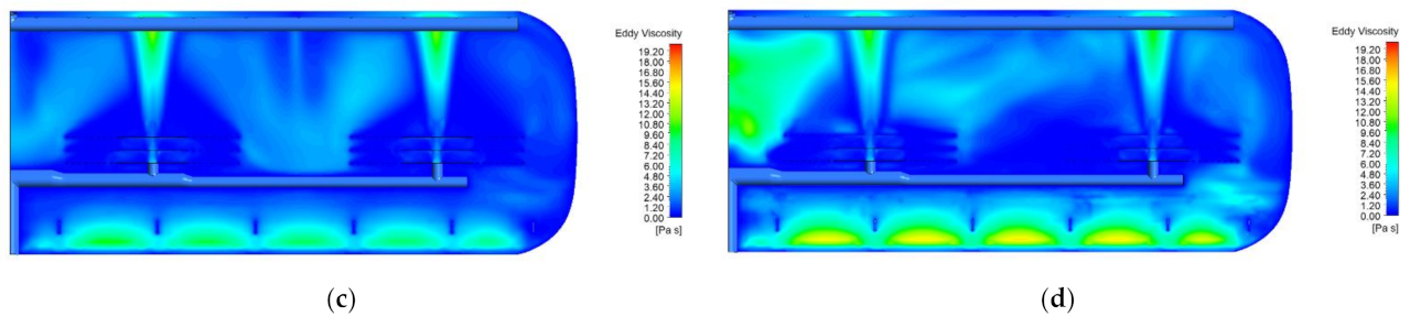
3.1. Hydrodynamic Analysis

From Figure 7, it is possible to explain the behavior presented in Figure 3 and Figure 5 on the oil volume fraction or separation of oil from water, where the effects of the electric field and water content are analyzed, which are the most significant variables in the process. It is concluded that the separation is significantly improved by raising the electric field from 0.1 kV/cm to 3 kV/cm. By examining Figure 7c,d with electric fields of 3 kV/cm and 0.1 kV/cm, respectively, it can be seen that at 3 kV/cm, the turbulence is much lower than in the case of 0.1 kV/cm. A similar trend is found in Figure 7a,b with a water content of 0.12 and 0.03, respectively, where the turbulence is much lower in the case of better separation (x = 0.12) than in the case of worst separation (x = 0.03), showing high turbulence. These results suggest that turbulence promotes collision and prevents the coalescence of oil droplets. Then, moderate turbulence is required to encourage collisions but not too much to allow the coalescence of droplets.

Further explanation about the differences in the separation obtained by changing the water content and the electric field comes from Figure 8, where the effect of the electric field and water content on the liquid velocity field is analyzed. In all cases, basic features of the flow field are the vertical high-velocity flow coming from the inlets, a clockwise circulation at the right lateral wall, and a low-velocity zone below the water outlets. In a high electric field of 3 kV/cm (Figure 8c), two well-defined circulation loops appear in the center of the desalter that are not defined at low electric fields of 0.1 kV/cm (Figure 8d). In the case of the high water content of x = 0.012 (Figure 8a), these circulations in the center are present but not at low water content (Figure 8b). These circulation loops seem to increase the residence time of oil droplets that help in the separation process, although the residence time curves were not considered in this work.

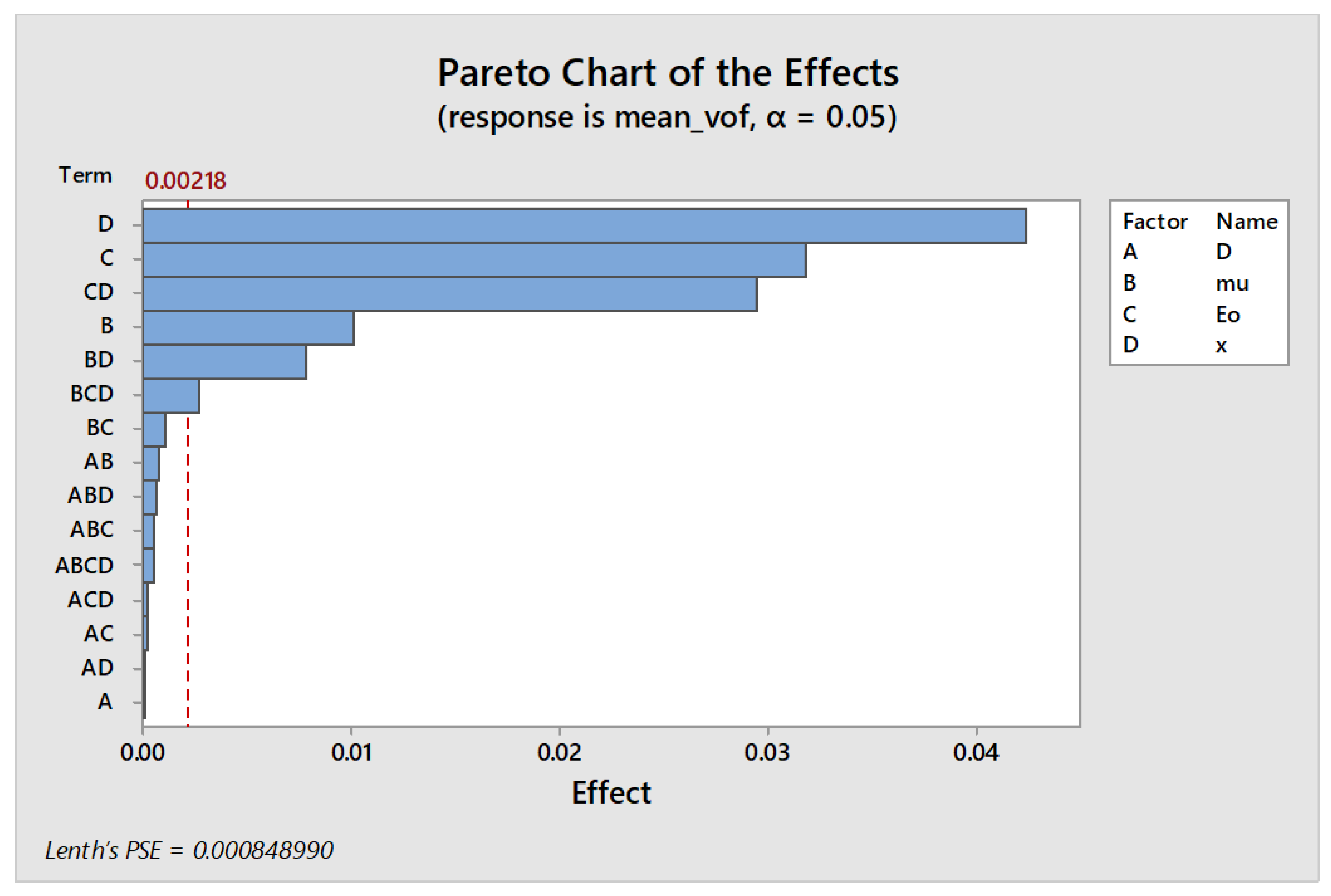
3.2. Statistical Analysis and Optimization

Table 7. Analysis of Variance.

Term	Effect	Coefficient	Std Dev.	p-Value
µ	0.010134	0.005067	0.000656	0.001
E	−0.03191	−0.01596	0.000656	0.000
X	0.04239	0.02119	0.000656	0.000
µ × x	0.007805	0.003903	0.000656	0.002
E × x	−0.02950	−0.01475	0.000656	0.000

shows the statistical analysis of each main effect of the four variables, along with double effects. Figure 9 shows a Pareto graph where the single results are reported along with double and triple interactions and the statistical significance through a dashed line. All effects lower than this line may be considered statistically insignificant and are, consequently, not reported in Table 7.

Table 7 and Figure 9 clearly state that only three variables and two double interactions are significant in oil separation. These are from high to low effects: water content, electric field, the combined effect of water content–electric field, and oil viscosity (temperature). If the initial water content increases from 0.03 to 0.12, water separation decreases by 4.24%. Aryafard et al. [14,15] found a similar improvement of oil content at the outlet from 96 to 98.5% when wash water is changed from 3 to 6% and validated in an industrial unit. Supposing the electric field increases from 0.1 kV/cm to 3 kV/cm, the separation of salty water is enhanced by 3.2%. Not too many studies are clear on the effect of the electric strength. Aryafard [14] et al. showed that increasing the electric field from 1.5 to 2 kV/cm increases the water removal efficiency from 96.4% to 97.8% in the crude oil. The effect of the combination of water content and the electric field is interesting, which indicates that a simultaneous increment in water and the electric field is beneficial by 3% separation. Finally, the increment in viscosity from 0.017 kg/ms to 0.071 kg/ms diminishes water separation from the oil by almost 1%. The droplet size resulted as insignificant. However, in the real process, this variable is linked somehow to the amount of fresh water in the desalting unit. Thus, the true nature of the simulation does not distinguish a case with high water content and small droplet size from a case with high water content and small droplet size. One of these two conditions may be challenging to meet in a real desalter. In the literature, many authors point out that the droplet size is essential as its size dominates the forces acting on the droplet that causes the collision and coalescence process needed for the separation [10,13,14].

The statistical analysis allowed us to obtain a response surface of the final water content at the oil outlet as a function of the main variables explored and expressed through the following equation not including the insignificant terms as:

$$\mathrm{Mean} \mathrm{Volume} \mathrm{Water} \mathrm{Fraction}=0.01041-0.1221\mathsf{\mu } +0.003830\mathrm{E}+0.6304\mathrm{x}+4.373\mathsf{\mu }\times \mathrm{x} -0.1865\mathrm{E}\times \mathrm{x}$$

(1)

The above equation was used to obtain a formal optimization analysis through the genetic algorithm built in the optimization module of MATLAB. The optimization consisted in minimizing the water content at the oil outlets, i.e., maximizing the separation of water from the crude oil. The outcome of this optimization exercise is the recognition of 25 optimum conditions (Pareto front) described in

Table 8. Pareto front with optima.

Optimum Point	D	μ	E	x	Mean Volume Fraction of Water
1	3.06095597	0.01707254	2.99339092	0.03003833	0.02526776
2	3.52471021	0.01701073	2.99998767	0.03001266	0.02524942
3	3.55716842	0.01703218	2.98611306	0.03003497	0.02527249
4	6.1115551	0.01701526	2.99889999	0.03004764	0.02524273
5	7.33734703	0.01701039	2.9964797	0.03003354	0.02523891
6	7.7335968	0.01704495	2.99988084	0.03008657	0.0252396
7	7.83882932	0.01704015	2.94999207	0.03003251	0.0253042
8	8.06589326	0.01707272	2.91442089	0.03008012	0.02536068
9	8.52232293	0.0170021	2.99859394	0.03000871	0.02522771
10	10.0636939	0.01710667	2.99625853	0.03005619	0.0252359
11	10.2583472	0.01702999	2.96275447	0.03005567	0.02527663
12	10.3801102	0.01704703	2.99860591	0.03009518	0.02523013
13	11.7521461	0.01704481	2.99105772	0.03001022	0.02522692
14	12.2213506	0.01702969	2.98366032	0.03006916	0.02523927
15	12.4154352	0.01703886	2.99939996	0.03004532	0.02521476
16	12.9440779	0.01701494	2.99693118	0.03003288	0.02521299
17	13.0555521	0.01702826	2.90428816	0.03000283	0.02534075
18	13.6925743	0.01700749	2.97734302	0.03003171	0.0252365
19	13.70686	0.0170153	2.99584673	0.0300342	0.02521118
20	15.5920049	0.01707421	2.97423509	0.03002545	0.0252366
21	16.5123639	0.01700549	2.99958726	0.03006071	0.02519454
22	16.6602285	0.01708459	2.99414794	0.03002029	0.02520413
23	17.0696906	0.01700989	2.98707433	0.03003351	0.02520774
24	18.7182166	0.01700966	2.98791986	0.03000627	0.02519679
25	18.8514308	0.01704943	2.9998606	0.03006069	0.02518672

.

From the optimum variables presented in Table 8, the previous analysis can be confirmed through the comparison of the oil volume fraction contours, where the effect of every variable was discussed. Then, the optimum conditions under the range of values explored in this study are (a) electric field of 3 kV/cm, (b) high temperature with an oil viscosity of 0.017 kg/ms, and (c) initial water content of 3%, and the size of the droplet that has no effect may vary from 19 to 3 µm, ratifying that this variable showed no effect on the separation. All these conditions indicate a final water content of 2.5%, as can be seen in the last column in Table 8, where the optimum water content at the oil outlets is presented as the optimum value. Comparison against other studies is difficult because the variables are not the same and because there are only a few optimization studies. For instance, Mahdi et al. [8] reported optimum values of a demulsifying agent concentration of 15 ppm, temperature of 77 °C, 10% wash water dilution ratio, settling time of 3 min, and mixing time of 9 min. Aryafard [14] et al. proposed the following increments in the electric field from 1.5 to 2 kV/cm, wash water from 3% to 6%, and pressure drop from 20 to 30 psi.

4. Conclusions

The statistical analysis indicated that the most significant variables affecting the water separation from oil were from higher to lower impact: the water content, the electric field intensity, and the oil viscosity. At the same time, the droplet size was insignificant in the separation under the conditions explored in this work. Increasing the electric field and decreasing the water content and oil viscosity (increasing temperature), better separation is achieved. It was found that the excess turbulence promotes collisions but may prevent actual coalescence and, therefore, it does not help in the separation. Additionally, it was found that the many circulation loops found in the cases of high electric fields and low water content may increase the residence time of the droplets, giving enough time for better separation than in the cases of low electric fields and high water content. Optimum values suggested from the optimization are E0 = 3 kV/cm, µ = 0.017 kg/ms, and water content of 3%.

References

1. Lovell, J. Climate report calls for green ‘New Deal’. Reuters 2008. [Google Scholar]
2. Chohan, U.W. A Green New Deal: Discursive Review and Appraisal. Notes on the 21st Century (CBRI). Notes 21st Century CBRI 2019. [Google Scholar] [CrossRef]
3. Varadaraj, R.; Savage, D.W.; Brons, C.H. Chemical Demulsifier for Desalting Heavy Crude. U.S. Patent 6,168,702, 28 January 2001. [Google Scholar]
4. Alshehri, A. Modeling and Optimization of Desalting Process in Oil Industry. Master’s Thesis, University of Waterloo, Waterloo, ON, Canada, 2009; p. 74. [Google Scholar]
5. Abdel-Aal, H.K.; Aggour, M.A.; Fahim, M.A. Petroleum and Gas Field Processing; CRC Press: Boca Raton, FL, USA, 2003. [Google Scholar]
6. Al-Otaibi, M.B.; Elkamel, A.; Nassehi, A.V.; Abdul-Wahab, S.A. A Computational Intelligence Based Approach for the Analysis and Optimization of a Crude Oil Desalting and Dehydration Process. Energy Fuels 2005, 19, 2526–2534. [Google Scholar] [CrossRef]
7. Sams, G.W.; Zaouk, M. Emulsion Resolution in Electrostatic Processes. Energy Fuels 1999, 14, 31–37. [Google Scholar] [CrossRef]
8. Mahdi, K.; Gheshlaghi, R.; Zahedi, G.; Lohi, A. Characterization and modeling of a crude oil desalting plant by a statistically designed approach. J. Pet. Sci. Eng. 2008, 61, 116–123. [Google Scholar] [CrossRef]
9. Herrmann, H.; Bucksch, H. Mud Logging. In Dictionary Geotechnical Engineering/Wörterbuch GeoTechnik; Springer: Berlin/Heidelberg, Germany, 2014. [Google Scholar] [CrossRef]
10. Bresciani, A.E.; Alves, R.M.B.; Nascimento, C.A.O. Coalescence of Water Droplets in Crude Oil Emulsions: Analytical Solution. Chem. Eng. Technol. 2010, 33, 237–243. [Google Scholar] [CrossRef]
11. Pruneda, E.F.; Rivero, E.; Escobedo, B.; Javier, F.; Vázquez, G. Optimum Temperature in the Electrostatic Desalting of Maya Crude Oil. J. Mex. Chem. Soc. Vol. 2005, 49, 14–19. [Google Scholar]
12. Wilkinson, D.; Waldie, B.; Nor, M.I.M.; Lee, H.Y. Baffle plate configurations to enhance separation in horizontal primary separators. Chem. Eng. J. 2000, 77, 221–226. [Google Scholar] [CrossRef]
13. Bresciani, A.E.; Mendonça, C.F.; Alves, R.M.; Nascimento, C.A. Modeling the kinetics of the coalescence of water droplets in crude oil emulsions subject to an electric field, with the cellular automata technique. Comput. Chem. Eng. 2010, 34, 1962–1968. [Google Scholar] [CrossRef]
14. Aryafard, E.; Farsi, M.; Rahimpour, M.; Raeissi, S. Modeling electrostatic separation for dehydration and desalination of crude oil in an industrial two-stage desalting plant. J. Taiwan Inst. Chem. Eng. 2016, 58, 141–147. [Google Scholar] [CrossRef]
15. Aryafard, E.; Farsi, M.; Rahimpour, M.R. Modeling and simulation of crude oil desalting in an industrial plant considering mixing valve and electrostatic drum. Chem. Eng. Process. Process Intensif. 2015, 95, 383–389. [Google Scholar] [CrossRef]
16. Kakhki, N.A.; Farsi, M.; Rahimpour, M.R. Effect of current frequency on crude oil dehydration in an industrial electrostatic coalescer. J. Taiwan Inst. Chem. Eng. 2016, 67, 1–10. [Google Scholar] [CrossRef]
17. Vafajoo, L.; Ganjian, K.; Fattahi, M. Influence of key parameters on crude oil desalting: An experimental and theoretical study. J. Pet. Sci. Eng. 2012, 90, 107–111. [Google Scholar] [CrossRef]
18. Bansal, H. Ameensayal. CFD Analysis of Horizontal Electrostatic Desalter-Influence of Header Obstruction Plate Design on Crue-Water Separation. 2015. Available online: https://www.digitalxplore.org/up_proc/pdf/51-13951413061-6.pdf (accessed on 27 August 2022).
19. Shariff, M.M.; Oshinowo, L.M. Debottlenecking Water-Oil Separation with Increasing Water Flow Rates in Mature Oil Fields. In Proceedings of the 5th Water Arabia 2017 Conference and Exhibition, Al-Khobar, Saudi, 17 October 2017; pp. 17–19. [Google Scholar]
20. Alhajri, N.A.; White, R.J.; Oshinowo, L.M. High Efficiency Static Mixer Technology for Crude Desalting. In Proceedings of the SPE Kingdom of Saudi Arabia Annual Technical Symposium and Exhibition, Dammam, Saudi Arabia, 23–26 April 2018; SPE-192388-MS. OnePetro: Richardson, TX, USA, 2018. [Google Scholar] [CrossRef]
21. Favero, J.L.; Silva, L.F.L.; Lage, P.L. Modeling and simulation of mixing in water-in-oil emulsion flow through a valve-like element using a population balance model. Comput. Chem. Eng. 2015, 75, 155–170. [Google Scholar] [CrossRef]
22. Wang, F.; Wang, L.; Chen, G.; Zhu, D. Numerical Simulation of the Oil Droplet Size Distribution Considering Coalescence and Breakup in Aero-Engine Bearing Chamber. Appl. Sci. 2020, 10, 5648. [Google Scholar] [CrossRef]
23. Sofos, F. A Water/Ion Separation Device: Theoretical and Numerical Investigation. Appl. Sci. 2021, 11, 8548. [Google Scholar] [CrossRef]
24. Shi, Y.; Chen, J.; Pan, Z. Experimental Study on the Performance of a Novel Compact Electrostatic Coalescer with Helical Electrodes. Energies 2021, 14, 1733. [Google Scholar] [CrossRef]
25. Sellman, E.; Sams, G.W.; Mandewalkar, S.P.K. Improved Dehydration and Desalting of Mature Crude Oil Fields. In Proceedings of the SPE Middle East Oil and Gas Show and Conference, Manama, Bahrain, 10 March 2013. [Google Scholar] [CrossRef]
26. Ramirez-Argaez, M.; Abreú-López, D.; Gracia-Fadrique, J.; Dutta, A. Numerical Study of Electrostatic Desalting Process Based on Droplet Collision Time. Processes 2021, 9, 1226. [Google Scholar] [CrossRef]
27. Dutta, A.; Ramírez-Argáez, M.A. Modeling of an Industrial Electrostatic Desalting Unit Using Computational Fluid Dynamics (CFD). Scıentıfıc Conference “Scıence, Technology and Development of Innovatıve Technologıes”. In Proceedings of the 30th Annıversary of Independence of Turkmenıstan, Ashgabat, Turkmenistan, 12–13 June 2021. [Google Scholar]
28. Pericleous, K.A.; Drake, S.N. An Algebraic Slip Model of Phoenics for Multi-phase Applications. In Numerical Simulation of Fluid Flow and Heat/Mass Transfer Processes; Springer: Berlin/Heidelberg, Germany, 1986; pp. 375–385. [Google Scholar] [CrossRef]
29. Kar, S.; Majumder, S.; Constales, D.; Pal, T.; Dutta, A. A comparative study of multi objective optimization algorithms for a cellular automata model. Rev. Mex. Ing. Quim. 2019, 19, 299–311. [Google Scholar] [CrossRef] [Green Version]
Figure 1. Schematic of the desalting unit used in this study.
Processes 10 02118 g001
Figure 2. Optimal mesh design, after performing a grid sensitivity study, indicating a semi-structured grid with 3.4 million cells. Note that the mesh represents only half of the schematic shown in Figure 1 due to the symmetry of the system.
Processes 10 02118 g002
Figure 3. Effect of the electric field on the oil volume fraction in a longitudinal plane for (a) high electric field, experiment 11 (D = 1 µm, µ = 0.071 kg/ms, x = 0.12, and E = 3 kV/cm); (b) low electric field, experiment 15 (D = 1 µm, µ = 0.071 kg/ms, x = 0.12, and E = 0.1 kV/cm).
Processes 10 02118 g003
Figure 4. Effect of the temperature (oil viscosity) on the oil volume fraction in a longitudinal plane for (a) high viscosity, experiment 12 (D = 20 µm, µ = 0.071 kg/ms, x = 0.12, and E = 0.1 kV/cm); (b) low viscosity, experiment 10 (D = 20 µm, µ = 0.017 kg/ms, x = 0.12, and E = 0.1 kV/cm).
Processes 10 02118 g004
Figure 5. Effect of the water content on the oil volume fraction in a longitudinal plane for (a) high water content, experiment 9 (D = 1 µm, µ = 0.017 kg/ms, x = 0.12, and E = 0.1 kV/cm); (b) low water content, experiment 1 (D = 1 µm, µ = 0.017 kg/ms, x = 0.03, and E = 0.1 kV/cm).
Processes 10 02118 g005
Figure 6. Effect of the droplet size on the oil volume fraction in a longitudinal plane for (a) high droplet size, experiment 6 (D = 20 µm, µ = 0.017 kg/ms, x = 0.03, and E = 3 kV/cm); (b) low droplet size, experiment 5 (D = 1 µm, µ = 0.017 kg/ms, x = 0.03, and E = 3 kV/cm).
Processes 10 02118 g006
Figure 7. Effect of the water content on the Eddy viscosity in a longitudinal plane for (a) high water content, experiment 9 (D = 1 µm, µ = 0.017 kg/ms, x = 0.12, and E = 0.1 kV/cm); (b) low water content, experiment 1 (D = 1 µm, µ = 0.017 kg/ms, x = 0.03, and E = 0.1 kV/cm). Effect of the electric field on the Eddy viscosity in a longitudinal plane for (c) high electric field, experiment 11 (D = 1 µm, µ = 0.071 Kg/ms, x = 0.12, and E = 3 kV/cm); (d) low electric field, experiment 15 (D = 1 µm, µ = 0.071 Kg/ms, x = 0.12, and E = 0.1 kV/cm).
Processes 10 02118 g007aProcesses 10 02118 g007b
Figure 8. Effect of the water content on the velocity in a longitudinal plane for (a) high water content, experiment 9 (D = 1 µm, µ = 0.017 kg/ms, x = 0.12, and E = 0.1 kV/cm); (b) low water content, experiment 1 (D = 1 µm, µ = 0.017 kg/ms, x = 0.03, and E = 0.1 kV/cm). Effect of the electric field on the velocity in a longitudinal plane for (c) high electric field, experiment 11 (D = 1 µm, µ = 0.071 kg/ms, x = 0.12, and E = 3 kV/cm); (d) low electric field, experiment 15 (D = 1 µm, µ = 0.071 kg/ms, x = 0.12, and E = 0.1 kV/cm).
Processes 10 02118 g008
Figure 9. Pareto chart of the single effects, namely pressure drop at the inlet valve (droplet size, D), content of freshwater x, temperature (viscosity of the oil µ), and electric field E. In addition, effects of double, triple, and quadruple interactions are shown.
Processes 10 02118 g009