
Analysis of Potential Fluctuation in Flow

Department of Energy Engineering, Yuquan Campus, Zhejiang University, 38 Zheda Road, Hangzhou 310027, China
Processes 2022, 10(10), 2107; https://doi.org/10.3390/pr10102107
Submission received: 11 September 2022
/
Revised: 10 October 2022
/
Accepted: 12 October 2022
/
Published: 17 October 2022
(This article belongs to the Section Chemical Processes and Systems)
Abstract
Understanding the physics of flow instabilities is important for processes in a wide range of engineering applications. Flow instabilities occur at the interfaces between moving fluids. Potential fluctuations are generated at the interfaces between two moving fluids based on the relationship of continuity. Theoretical analysis demonstrated that, in flow instabilities, potential fluctuation exhibits a potential oscillatory wave surface concurrently in the temporal and spatial dimensions. Potential fluctuations already internally exist in flow before flow instabilities begin to develop; these potential fluctuations greatly affect the formation of interpenetrating structures after forces act on the interfaces. Experimental studies supported the theoretical study: Experiments visualizing condensation flows using refrigerant in one smooth tube and one three-dimensional enhanced tube were conducted to show the development of potential fluctuation in spatial dimensions, and an experiment with cooling tower fouling in seven helically ridged tubes and one smooth tube were conducted to show the development of potential fluctuation in the temporal dimension. Both experimental studies confirmed that potential fluctuation was determined by the densities and velocities of the two fluids in the instability as indicated by the relationship of continuity. In addition, the results of numerical simulation in the literature qualitatively confirm the theoretical study. This paper is a first attempt to provide a comprehensive analysis of the potential fluctuation in flow.
1. Introduction
Flow instabilities occur at the interfaces among moving fluids. This research effort began with the landmark work of L. Rayleigh, followed by its modern development by G.I. Taylor. Rayleigh–Taylor instability (RTI) occurs whenever a lighter fluid of density supports a heavy fluid of density against gravity. Richtmyer–Meshkov instability (RMI) is the impulsive acceleration limit of RTI. The RMI arises when a shock passes through an interface between two fluids. Kelvin–Helmholtz instability (KHI) occurs whenever shear velocity presents within a continuous fluid or when a sufficient velocity difference exists across the interface between two fluids. The RTI, KHI, and RMI are all referred to as flow instabilities in this study [1,2,3,4].
Flow instabilities are triggering events that lead to fluid mixing in electro-hydro-dynamical and many other industrial processes. The slightest initial perturbation at the interface leads to tangential acceleration and is amplified by material flowing down under the influence of forces which are magnified in a variety of interpenetrating structures. Initial perturbations and interpenetrating structures are the structures/appearances of flow instabilities in the initial stage and the developed stage, respectively. Previous studies have focused on the influence of forces, for instance, surface tension, elasticity, ablation, viscosity, accretion, plasticity, and other effect-causing forces, on the interface. Cook and Zhou [5] provided visualizations of the stages of RTI growth by using direct numerical simulation (DNS). The initial density perturbations were depicted in snapshots; the flow is seeded with fine-scale perturbations. Figure 1 shows the time series of the density field. The images from left to right were taken at unit time = 1, 2, and 3, respectively. Heavy fluid is red, light fluid is blue, and mixed fluids are green. The early evolution is weakly nonlinear, characterized by the formation of upwardly rising bubbles of light fluid and downwardly penetrating heavy fluid spikes. Subsequently, bubbles and spikes begin to merge, and the flow becomes strongly nonlinear.
Inertial confinement fusion (ICF) determines the minimum energy required for ignition, which is a major concern when it comes to making fusion energy a viable alternative energy source. The RTI presents a serious design challenge for ICF capsules [6]. The spherical shell filled with low-density gas is composed of an outer region, which forms the ablator, and an inner region of frozen or liquid deuterium and tritium (DT), which forms the main fuel, as shown in Figure 2. The high-density shell is decelerated by the low-density fuel in the fusion chamber, depending on the ratio of shell radius to thickness. Laser-driven ICFs are either indirect drive (top left) or direct drive (top right). When the implosion reaches the minimum radius, the DT hot spot has formed and is surrounded by the cooler and denser DT fuel. The energy from the driver is quickly transferred to the ablator, which heats up and expands.
According to the surveyed literature, many researchers have paid attention to related issues of flow perturbations, such as pulsating flow. Wang et al. [7] studied the effect of pulsating free flow on the resistance of drag force and wake characteristics of stationary spherical particles using DNS. Sinusoidal fluctuation around a mean value is adopted as the freestream velocity. The reasons for this are that the basic assumptions of the point-particle model are not rigorously satisfied to reproduce the experimental results and the analysis of drag force acting on a particle in turbulent flow may result in prediction errors that cannot be ignored. The study of pulsating free flow for particles of finite size in turbulent flow is of great significance. Duan et al. [8] investigated the effect of flow-induced vibration using pulsating flow generated by a vortex generator on the heat transfer enhancement of a planar elastic tube bundle by adopting experimental and numerical methods in three kinds of flow fields. They found that heat transfer enhancement was obtained with a heat transfer coefficient increase of 28%, 25%, and 19.5% in pulsating flow, coupled flow, and steady flow, respectively. Wang et al. [9] applied particle image velocimetry and infrared thermography measurements to explore the effect of a quasi-triangular pulsatile flow inlet on heat transfer enhancement in a serpentine channel with winglike turbulators to enrich the understanding of pulsating flow and clarify its heat transfer mechanism. Selcuk [10] conducted a computational study to determine the effect of geometric improvements on an inferior vena cava filter with a helical flow inducer strut on blood flow hemodynamic properties and filter performance. The blood flow in the arterial system is pulsating. The properties of blood, including the density, were obtained by accounting for the nature of blood’s pulsatile flow.
Previous studies were about interpenetrating structures and initial perturbations of flow instabilities. Few research studies have been related to the origins of flow instabilities. The “inner gene” of instabilities has been ignored. This “inner gene” already exists internally before the instabilities begin to develop because of the universal conservation of mass. In the study, I propose that this is the potential fluctuation based on the continuity equation. Potential fluctuation’s influence on initial perturbation could be taken at a glance if the conditions are obtained. Conducting research on flow instability without investigating potential fluctuations is like conducting research on the evolution of life without investigating genes. This could result in incorrect approaches and directions, irrelevant factors and conditions, contradictory statements, conflict conclusions, and errors. The occurrence of the oscillatory wave interface of perturbation in flow is normal due to potential fluctuations. In other words, the interfaces of instabilities must be oscillatory in some way due to the continuity relation. After a variety of forces involved in the process act on the interface, initial perturbations develop into a variety of interpenetrating structures guided by potential fluctuations.
These important issues cannot be adequately covered without understanding potential fluctuation, and major developments were simply impossible until recently, when researchers acquired the ability to fabricate precise initial conditions, the diagnostics tools for the experiments, and sufficiently advanced supercomputing power. After several decades of effort, major breakthroughs have occurred in experiments, computation, and analysis. This paper brings these together, showing how observations from experimental measurements and numerical simulations, analytical treatments, and engineering models have been synthesized to describe the physics of flow instabilities. Understanding the physics of flow instabilities is of importance to processes in a wide range of scientific and engineering applications. This paper is aimed at filling the research gap regarding the origin of flow instability and interpenetrating structures by providing a comprehensive study including theoretical analysis, experimental verification, and numerical simulations. First, I presented a new theoretical analysis of potential fluctuation based on the continuity relation. Second, I conducted designed experimental studies on initial perturbations and interpenetrating structures to provide evidence for the theoretical analysis. Finally, I proposed the potential fluctuations of flow instabilities along the three space dimensions and one time dimension.
2. Theoretical Analysis
The analysis of potential fluctuation is as following: A control volume with density ρ at a point in flow is shown Figure 3A. ρ includes fluid ρ2 and fluid ρ1 (ρ2 ≠ ρ1). The continuity equation is:
The height of the interface between fluid ρ2 and fluid ρ1 is H as shown in Figure 3A. Both ρ2 and ρ1 are constants, Equation (1a) becomes:
Velocity v is a constant, Equation (2) is valid. Along the characteristic line , is a constant [11]. is the initial value. The solution of Equation (1b):
When a curve of the development of H exists, time period t of forming it had already passed; The “−” shall be included in Equation (3):
Therefore:
H (t, x) will satisfy Equation (1b) with the validation of Equation (3). Therefore:
where A, D, k and the initial value are constants. The potential fluctuation generated at the interfaces between two moving fluids is defined in Equation (5). It shows sinusoidal behavior along the spatial dimensions and the temporal dimension as shown in Figure 3B. This is the “inner gene” of flow instability. It is the origin of instabilities and has great influence on the development of interpenetrating structures after forces act on the interface. By modeling the interface that exists between the two fluids using boundary conditions for differential equations, a sinusoidal solution is obtained. There are infinite oscillatory solutions to this equation which thus form the basis on which any other type of solution can be represented. Sinusoidal solutions are associated with lower modes because they require less energy [11]. Potential fluctuations cannot be directly observed in the physical world because forces are required to move the liquid. After the forces act on the process, the underlying fluctuations develop into various interpenetrating structures depending on the various forces involved in the process.
Figure 3.
Sinusoidal interface between two fluids: (A) control volume at a point in flow; (B) potential fluctuation as given in Equation (5).
Figure 3.
Sinusoidal interface between two fluids: (A) control volume at a point in flow; (B) potential fluctuation as given in Equation (5).

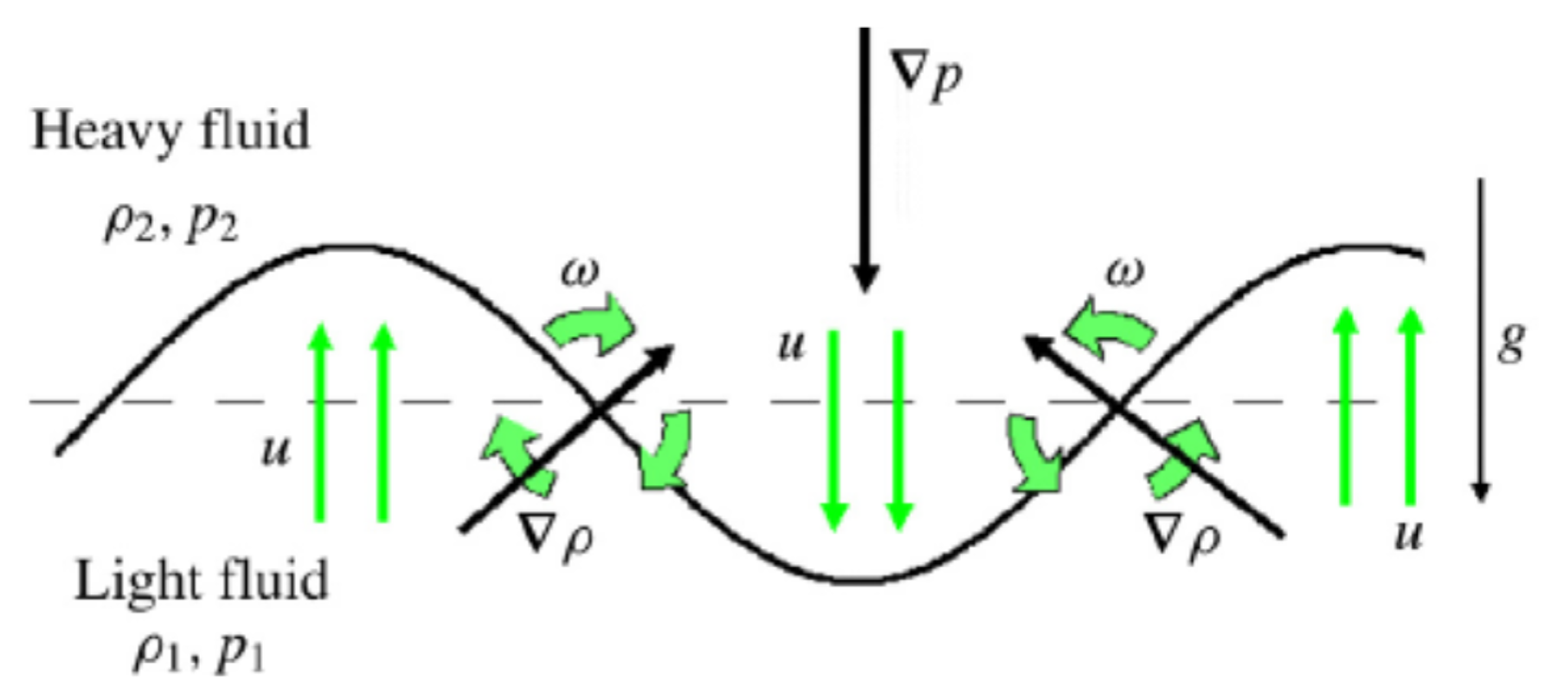
A sample figure of the initial interface perturbation of a flow instability with a sinusoidal wave as indicated in Equation (5) is shown in Figure 4, where g indicates gravity; p, pressure; ρ, density; ω, vorticity; and circular arrows represent the velocity field. If the heavy fluid pushes the light fluid, the interface is stable; however, if the light fluid pushes the heavy fluid, the interface is unstable. The interface becomes unstable with acceleration applied in the direction of the denser fluid [12].
The initial interface perturbation resulting from potential fluctuation at the very beginning of an instability has sinusoidal behaviors along the spatial and temporal dimensions simultaneously. A visual image of one individual initial interface perturbation in three spatial dimensions is shown in Figure 5 [4].
Potential fluctuation can be applied to the oscillatory phenomena of moving fluids in general flow instabilities (including but not limited to RTI, RMI, and KHI). Only the relationship of continuity is adopted in the development of Equation (5). The Newton’s second law of motion and the first law of thermodynamics are not adopted in the analysis. Introducing detailed boundary conditions is an analysis approach based on the momentum balance, and measuring accurate temperatures is an analysis approach based on the energy balance on the interface. However, accounting for all the factors makes the situation too complicated to be analyzed; it is an almost impossible mission because the experimental evidence of their effects on flow instabilities cannot be directly established with the present scientific testing capability [6]. Figure 4 and Figure 5 present pictures of the initial interface perturbation to qualitatively support the theoretical analysis. Analysis that advances new theoretical views needs to contain specific experimental evidence that the interpretations are distinguishable from existing knowledge. Visualization experiments using refrigerant as a work fluid during condensation flows in a smooth tube and a three-dimensional enhanced tube were conducted to show the development of potential fluctuation in in spatial dimensions. Cooling tower fouling in seven helically ridged tubes and one smooth tube were conducted to obtain information on the sinusoidal behavior of the interface between two mediums with a tiny density difference to show the development of potential fluctuation in the temporal dimension. Based on previous studies and with the goal of avoiding their shortcomings, two unique experimental approaches are advanced to provide evidence for the analysis of potential fluctuation in the next section.
3. Experimental Evidence
3.1. Development of Potential Fluctuation in Spatial Dimensions
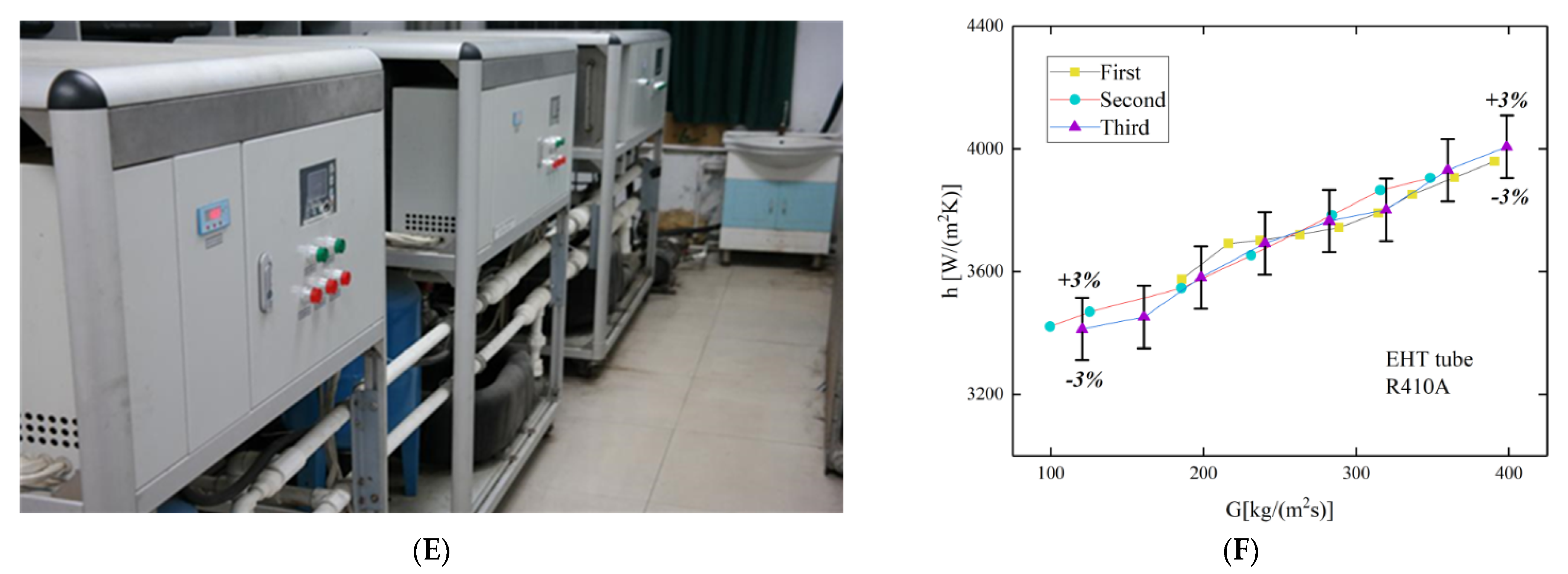
Figure 6A shows a schematic of the experimental facility used in the study. A high-precision bench suitable for condensation heat transfer experiments in tubes with various working fluids such as R410A, R32, and R134a was used. A two-phase heat exchange test section consisted of a refrigerant circulation loop and a water circulation loop. Driven by a digital variable frequency pump, the refrigerant entered a preheating section equipped with a smart temperature control system, where the refrigerant was heated. In the test section, a countercurrent sleeve heat exchanger was used for condensation experiments, as shown in Figure 6B. The effective heat transfer length of the test section was 2.0 m, and a copper tube with an outer diameter of 17.0 mm was selected as the external tube. An enhanced tube with internal petal-like protrusions and staggered dimples (EHT tube) is a complex interior surface tube on the market [12] as shown in Figure 6C. Visualizations of flow patterns of condensation flow using refrigerant R410A in smooth and EHT tubes with a diameter of 12.7 mm were conducted. Geometric parameters for the two tested tubes are listed in Table 1 During the flow condensation experiments, the refrigerant flowed across the tested tubes while the cooling water flowed through the annulus and cooled the refrigerants. The refrigerant flowed from right to left inside a tested tube, and deionized water flowed from left to right in the outer annular region of the tested tube. The exterior of the test section was wrapped with a layer of polyurethane sealant foam, a polyethylene plastic pipe, and a layer of rubber thermal insulation cotton for thermal insulation purposes. Figure 6D,E shows the physical diagram of the test bench. The test facility, experimental data reduction, and repeat condensation flow heat transfer experiments for validation are described in detail in Sun et al. [13]. The experiment was conducted at a saturation temperature of 318 K, an outlet vapor quality from 0.1 to 0.9, and at refrigerant R410A mass fluxes of 100 kg/(m2s). To validate the accuracy of the experimental results, the condensation flow tests of the EHT tube were conducted three times. The experimental results of the heat transfer coefficient for the three times were reproducible within a random error band of ±3% as shown in Figure 6F, which shows that the experimental data have good reproducibility. The uncertainty of the in-tube heat transfer coefficient is 10.2%, which shows a high test accuracy [13].
The visualization section was installed at the export of the test section to observe the condensation flow patterns in a smooth tube and an EHT tube, respectively. By minimizing the diameter difference between the tested tube and the quartz glass tube used for observation in the visualization section, possible turbulence caused by sudden expansion or contraction was avoided. Figure 7 shows a schematic diagram of the image acquisition device. At the central axis between the two stainless steel flanges, a 10 mm quartz glass tube served as a sight glass for flow visualization. Extending from the flange to both sides were stainless steel hex female fittings, reducing hex fittings and hollow nuts welded to the flange. In addition, two copper tubes with a 12.7 mm outside diameter were seamlessly welded to the scope body and the test tube. A Phantom VEO-1010 high-speed camera was utilized to capture the condensation flow patterns with an image acquisition frequency of 4000 fps and a resolution of 1280 × 960 pixels.
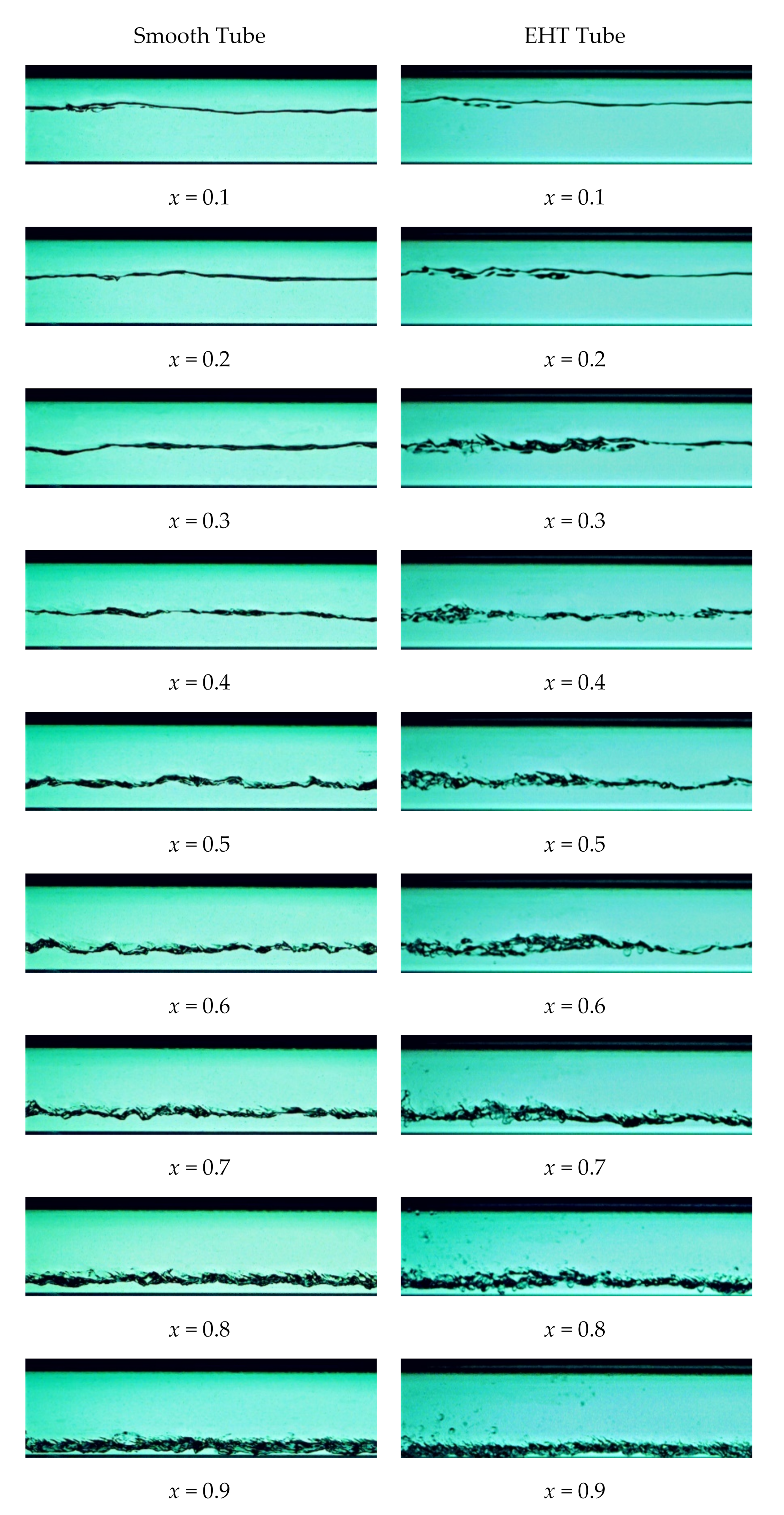
Condensation flow patterns inside smooth and EHT horizontal tubes are shown for comparison in Figure 8. At x = 0.1, both examples of the approximate appearance of initial interface perturbation in the shape of the sinusoidal function inside the two tubes caused by potential fluctuation defined in Equation (5) are images of refrigerant R410A vapor blowing over an R410A liquid surface. In this situation, the vapor caused a relative motion between the stratified interface of liquid and vapor. Vapor velocity increased as vapor quality x progressed from 0.1 to 0.9 in the tested tube, enlarging the influence of vapor shear on the condensate. Large magnitude waves were produced, as observed in stratified wavy flows with increasing vapor quality. The initial interface perturbations (for an example, at x = 0.1) manifest themselves through vapor shears into the form of interpenetrating structures (for an example, at x = 0.9) being generated on the liquid surface; these are the result of flow instabilities between liquid and vapor. The flow rate of the refrigerant flowing through the smooth tube and the EHT tube is the same, at refrigerant R410A mass fluxes of 100 kg/(m2s). Under the same vapor quality of the condensing flow, the refrigerant liquid flow velocity in the smooth tube and in the EHT tube is the same, and the flow velocity of the refrigerant vapor in the two tubes is the same. Thus, the difference between the relative flow velocity of the refrigerant liquid and the vapor in the smooth tube and the EHT tube is also the same. Comparing the photos of the refrigerant flow patterns in the smooth tube and the EHT tube under the same vapor quality in Figure 8, one can see that there is not much difference in the flow patterns between the two photos. Further, in the comparison of the flow patterns between the two columns in Figure 8, one can observe a good agreement between the flow patterns in the smooth tube and the flow patterns in the EHT tube of the same vapor quality in the same row. The results of the experimental observations are consistent with the inferences of Equation (5). It seems that the double layer enhancement surface of the EHT tube has little effect on the flow patterns. Surface topography alters shear stresses at the tube wall instead of the shear stresses on the condensate. In general, surface topography has little effect on initial interface perturbation and interpenetrating structures because initial interface perturbation and interpenetrating structures are primarily controlled by the potential fluctuation. Potential fluctuation is determined by ρ1, v1 and ρ2, v2 of the two fluids as determined by the relation of continuity.
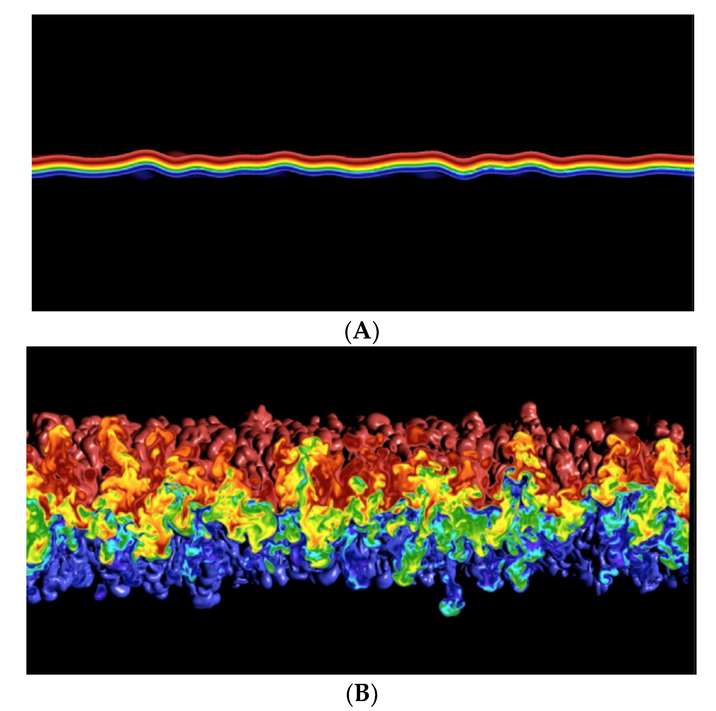
Cabot and Cook [14] show snapshots of density field evolution from DNS of RTI in the fully turbulent regime. The heavy fluid is red, the light fluid is blue, and the mixed fluid is green. The flows are initialized with a stationary interface between the high and low-density fluids, whose vertical position is perturbed with potential fluctuations having a characteristic horizontal wavelength that act to seed the instability. The initial interface perturbations are shown in Figure 9A. The simulations proceeding to interpenetrating structures, with the mixing layer filling 50% of the domain in the vertical direction, are shown in Figure 9B. Figure 8 and Figure 9 present the visualization of the development of initial interface perturbations to interpenetrating structures of flow instability in spatial dimensions by experimental study and DNS, respectively.
3.2. Development of Potential Fluctuation in the Temporal Dimension
Fouling deposits in cooling tower water can provide the appearance of initial interfacial perturbation. The density ρ2 of the fouling layer (fouling sediment particles and water) is greater than the density ρ1 of the fluid (water only) above the fouling layer. The fouling layer and water provide the density and velocity differences needed to observe flow instabilities on the fouling layer surface. As shown in Figure 10A, a test shell-and-tube condenser was installed parallel with the condenser of a 900-kW chiller in a newly built structure on campus. The cooling tower water supplied to the main refrigerant condenser was supplied to the tested tubes in the condenser. The condenser contained sixteen tubes 3.7 m in length installed as eight identical pairs (seven pairs of helical ridge tubes and one pair with smooth tube geometry). The rationale for pairing is to have one of the tubes in a pair operate as a fouling-free control and have the other tube experience chronic fouling. Tubes are paired horizontally to minimize local differences on the condensate outflow side of the tubes. All eight tubes have an inner tube diameter of 15.54 mm and are made with 1024 fins/inch (0.90 mm high) on the outer surface, as shown in Figure 10B. The internal geometric parameters of the helical spine tube ranged from the rib start number, helix angle and height defined in Table 2. Tube 1 is a smooth tube for comparison with the other seven helical spine tubes.
The thermal resistance of the fouling layer was obtained by taking the difference between the heat transfer coefficients of the fouled tube and clean tube in a pair. The tests were carried out under the following operating conditions: Cooling tower water circulated through the tested condenser in a single pass arrangement at a tube side velocity of 1.07 m/s (Re = 16,000). Typical operating conditions were 28.5 °C inlet water temperature, 32.5 °C outlet water temperature and 36.6 °C refrigerant condensation temperature. During a cooling season, data were collected every two days for more than 2570 h. These tests were performed over two cooling seasons in a row to confirm that the fouling data were repeatable [15]. After the experiment in one cooling season was done, foulant samples were removed and chemically analyzed. Analysis showed that 61% of the fouling deposits were calcium carbonate caused by precipitation fouling. The remaining 39% of the fouling deposits were amorphous particles, including silica (from rust, dirt particles, and sand from cooling air), copper oxide (from copper pipe), iron phosphate/silicate (from iron pipe), and silicic acid aluminum (from unidentified aluminum in the system). Analysis showed that a combination of precipitation and particulate fouling occurred in the experiments. An uncertainty analysis was performed [16]. Under typical chiller load condition at 4 °C water temperature rise, the experimental uncertainty in Rf is ±5.7 × 10⁶ m2 K/W. This uncertainty is 12% of the manufacturer’s condenser design rated fouling resistance Rf of ±4.4 × 10⁵ m2 K/W.
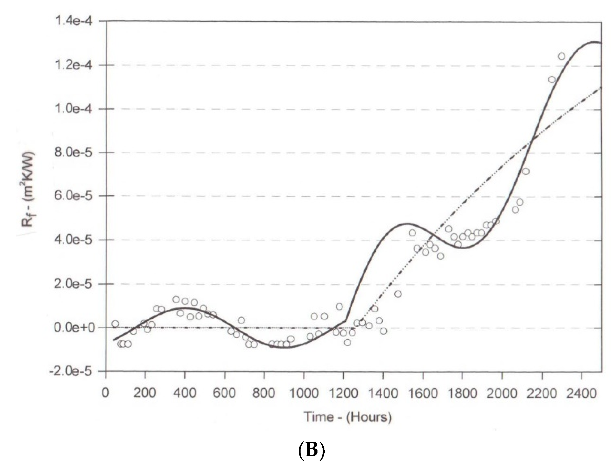
The transport of fouling particles in turbulent flow to the internal tube surface is responsible for the mass transfer of particles to the accumulation surface of a fouling deposit and is part of the combined mechanism of precipitation and particulate fouling. There are three transmission zones: the diffusion zone, the inertia zone, and the impact zone [17]. As the particles approach the surface, boundary layer effects must be considered. For particles smaller than about 10 μm, direct molecular diffusion across the boundary layer fully explains the experimental results; the particle size in this study is about 3.0 μm. Particle transport is in a diffuse zone. The particles move with the fluid and are brought to the wall by Brownian motion across the viscous sublayer. The micron particles may be regarded as macromolecules. The fouling layer is formed due to the deposition of suspended particles in flow. The density of the fouling layer (water and fouling deposit) is not the same as the density of the fluid (water). The water is above the fouling layer. The fouling layer and water provide the required density difference to observe the participating sinusoidal behavior on the fouling layer surface (the interface between the two densities) controlled by the potential fluctuations defined in Equation (5). Figure 11A shows cooling tower water fouling data for eight tested tubes. It shows the relationship between thermal resistance (Rf) and time (t) of the fouling layer. The eight curves all presented sinusoidal behavior [18]. The thermal resistance of the fouling layer was directly proportional to the thickness of the fouling layer. Therefore, the thickness of the fouling layers in the eight tested tubes presented sinusoidal curves as a function of time. The data in Figure 11A are almost overlapped with each other because the cooling tower water fouling data for the eight tested tubes are shown in one figure; the change law seems to be chaotic. To make it clear, the fouling data of Tube 2 is presented individually in Figure 11B. The figure clearly shows the sinusoidal curve. Figure 11 presents evidence of the development of potential fluctuation in the temporal dimension.
The curve of Tube 2 can be correlated by a sinusoidal function, Rf = Asin(λt) = 2.6 × 10⁵ sin(0.0072t). The temporal fluctuation amplitude (A) and temporal fluctuation cycle (λ) for all eight tested tubes are summarized in Table 2. As can be seen in the table, the temporal fluctuation cycle (λ) for the eight tested tubes is the same (λ = 0.072). This indicates that λ is not a function of the geometric parameters of the surface. This is because λ is a parameter of potential fluctuation defined by Equation (5). It is determined by ρ1, v1, and ρ2, v2, of the two fluids between the interface, which is the fouling deposit layer in this study, rather than the shear stresses of the tube wall. The temporal fluctuation cycle (λ) of the oscillatory interface between ρ1 and ρ2 has no relationship with the surfaces underneath ρ1 and ρ2 or the tube wall surfaces constraining the fluids of ρ1 and ρ2. As one can see in Table 2, the amplitude of the fluctuation (A) is a monotone decreasing function of axial element pitch/rib height (p/e), as is the fouling resistance ratio (Rf/Rfp). Rf/Rfp is directly proportional to the thickness of the fouling deposit in the tubes. The thicker the fouling deposit, the larger the amplitude of the fluctuation. Kern and Seaton’s fouling analysis has been a landmark in fouling research since in 1959; they assumed deposit accumulation is the result of two simultaneous opposing events, a constant deposition rate and an increasing removal rate. The removal rate is directly proportional to the thickness of the fouling deposit and the shear stress on the fouling deposit. The different thickness of the fouling deposits resulted in different values of A for the eight tested tubes. These differences are the result of different situations of shear stress in the eight tested tubes: The flow is interrupted by the rib, the boundary layer close to the wall is separated and then reattaches to the wall downstream of the rib when p/e > 5, and the reattachment point vanishes when p/e < 5, thus forcing the main flow to “glide over” the ribs and produce secondary flows between the ribs [19]. The amplitude of the fluctuation (A), a parameter of potential fluctuation, is affected by shear stresses of the tube wall. Figure 11 presents the evidence of the development of potential fluctuations in the temporal dimension.
Some studies on sinusoidal fouling curves in the literature include: (i) fouling data for an extended surface heat exchanger and a mass accumulation probe used in a diesel exhaust environment [20]; (ii) corrosion fouling [21]; (iii) magnetite particulate deposition from water flowing in aluminum tubes using an X-ray technique [22] as shown in Figure 12A; and (iv) the cooling tower water fouling performance of two types of brazed-plate heat exchangers (BPHEs) [23] in Figure 12B.
As one can see in Figure 12B, the wave asymptotic fouling curves for the fouling resistance of cooling tower water in two different brazed-plate heat exchangers (BPHE-1 and BPHE-2, each with a different plate surface) have the same values for λ because λ is not a function of the geometric parameters. Temporal wave fouling data, examples of which are shown in Figure 10 and Figure 11A,B, have been reported in the literature for more than 50 years; however, they have not yet been theoretically analyzed. Instead, researchers have focused on asymptotic fouling and have ignored temporal sinusoidal fouling due to the belief that its wave behavior was generated because of experimental uncertainty [16].
Figure 13, adopted from Ramaprabhu et al. [24], shows the three-dimensional dimensionless Froude numbers obtained for single mode perturbation for RTI. It is the result of numerical simulations. Figure 11 and Figure 13 present sinusoidal data of flow instabilities from experimental study and numerical simulations, respectively.
Visualization of condensation flows using refrigerant R410A in one smooth tube and one three-dimensional enhanced tube presents the development of potential fluctuation in spatial dimensions to show that the surface topography of the tube wall has little effect on initial interface perturbation and interpenetrating structures. Due to the limitation of diagnosis capability of the visualization of condensation flow, this method cannot provide detailed information on the spatial fluctuation amplitude and spatial fluctuation cycle of potential fluctuation. Cooling tower fouling in seven helically ridged tubes and one smooth tube present the development of potential fluctuation in the temporal dimension to further show that the surface topography of the tube wall has no effect on the temporal fluctuation cycle and has an obvious effect on temporal fluctuation amplitude due to change of shear stress situations caused by the surface topography of the tube wall.
The theoretical analysis is supported by experimental evidence as shown in Figure 8 and Figure 11, as well as previous studies as shown in Figure 9, Figure 12 and Figure 13. Based on visualization of condensation flows and cooling tower water fouling data, deductions can be reached. Potential fluctuation presents a sinusoidal interface in the spatial and temporal dimensions with A(x,y,z,t) and λ(x,y,z,t). The λ(x,y,z,t) and A(x,y,z,t) are primarily determined based on the densities (ρ1 and ρ2) and velocities (v1 and v2) of the two fluids involved in the flow instability. The value for A(x,y,z,t) is affected and λ(x,y,z,t) is not affected by the stresses caused by surface topography. Direct experimental evidence and quantitative analysis, with the advancement of diagnostic experimental tools and supercomputing power, are needed to obtain more specific information about potential fluctuation.
4. Conclusions
Potential fluctuations are generated at the interfaces between two moving fluids based on the relation of continuity. I conducted a theoretical analysis of potential fluctuation to demonstrate that potential fluctuation concurrently presents a potential oscillatory wave surface in the temporal and spatial dimensions in flow instabilities as defined by Equation (5). Potential fluctuation is determined by the two densities and two velocities of the two fluids in the instability, as indicated by the relation of continuity. Even before flow instabilities begin to develop, potential fluctuations already internally exist in flow. They are the origin of instabilities and have great influence on the development of interpenetrating structures after forces act on the interface.
I conducted visualization experiments during condensation flows using refrigerant in one smooth tube and one three-dimensional enhanced tube to investigate the development of potential fluctuation in spatial dimensions. Surface topography alters shear stresses at the tube wall and has little effect on initial interface perturbation and interpenetrating structures, which shows that potential fluctuation is primarily determined by ρ1, v1 and ρ2, v2 of the two fluids. I conducted cooling tower fouling experiments in seven helically ridged tubes and one smooth tube to further investigate the amplitude and wavelength of potential fluctuation in the temporal dimension. Amplitude and wavelength were determined based on the densities (ρ1 and ρ2) and velocities (v1 and v2) of the two fluids involved in the flow instability. Amplitude was affected and wavelength was not affected by the stresses caused by surface topography.
Both experimental studies support the theoretical analysis of potential fluctuation. The results of numerical simulation in the literature qualitatively confirm the theoretical study as well. This paper is a first attempt to provide a comprehensive analysis of the potential fluctuation in flow. Direct experimental evidence and quantitative analysis of potential fluctuation are needed in future investigations.
Funding
This work is supported by the National Science Foundation of China (52076187).
Acknowledgments
The author is deeply indebted to Professors: Jianhua Yan, Zhongyang Luo, Xiang Gao, ZitaoYu, Wei Zhong and Academician Kefa Cen in the Department of Energy Engineering in Zhejiang University in China for their support in the long journey of developing the analysis in the past sixteen years.
Conflicts of Interest
The authors declare no conflict of interest.
References
- Brouillette, M. The Richtmyer–Meshkov instability. Annu. Rev. Fluid Mech. 2002, 34, 445–468. [Google Scholar] [CrossRef]
- Hurricane, O.A.; Hansen, J.F.; Robey, H.F.; Remington, B.A.; Bono, M.J.; Harding, E.C.; Drake, R.P.; Kuranz, C.C. A high energy density shock driven Kelvin–Helmholtz shear layer experiment. Phys. Plasmas. 2009, 16, 056305. [Google Scholar] [CrossRef]
- Yabe, T.; Hoshino, H.; Tsuchiya, T. Two- and three-dimensional behavior of Rayleigh–Taylor and Kelvin–Helmholtz instabilities. Phys. Rev. A 1991, 44, 2756–2758. [Google Scholar] [CrossRef] [PubMed]
- Zhou, Y. Rayleigh-Taylor and Richtmyer-Meshkov instability induced flow, turbulence, and mixing. Phys. Rep. 2017, 723, 1–160. [Google Scholar]
- Cook, A.W.; Zhou, Y. Energy transfer in Rayleigh-Taylor instability. Phys. Rev. E 2002, 66, 026312. [Google Scholar] [CrossRef] [PubMed]
- Betti, R.; Hurricane, O.A. Hurricane, Corrigendum: Inertial-confinement fusion with lasers. Nat. Phys. 2016, 12, 435–448. [Google Scholar] [CrossRef]
- Wang, Y.; Zhu, Z.; Hu, R.; Shen, L. Direct numerical simulation of a stationary spherical particle in fluctuating inflows. AIP Adv. 2022, 12, 025019. [Google Scholar] [CrossRef]
- Duan, D.; Cheng, Y.; Ge, M.; Bi, W.; Ge, P.; Yang, X. Experimental and numerical study on heat transfer enhancement by Flow-induced vibration in pulsating flow. Appl. Therm. Eng. 2022, 207, 118–171. [Google Scholar] [CrossRef]
- Wang, C.S.; Chen, C.C.; Chang, W.C.; Liou, T.M. Experimental studies of turbulent pulsating flow and heat transfer in a serpentine channel with winglike turbulators. Int. Commun. Heat Mass Transf. 2022, 131, 105–837. [Google Scholar] [CrossRef]
- Selcuk, S. Investigation of helical strut attached vena cava filter hemodynamic performance. J. Eng. Res. 2021, 10, 174–183. [Google Scholar]
- Li, W. Two-phase heat transfer correlations in three-dimensional hierarchical tube. Int. J. Heat Mass Transf. 2022, 191, 122827. [Google Scholar] [CrossRef]
- Roberts, M.S.; Jacobs, J.W. The effects of forced small-wavelength, finite-bandwidth initial perturbations and miscibility on the turbulent Rayleigh-Taylor instability. J. Fluid Mech. 2016, 787, 50–83. [Google Scholar] [CrossRef]
- Sun, Z.C.; Li, W.; Ma, X.; Ma, L.X.; Yan, H. Transfer, Two-phase heat transfer in horizontal dimpled/protruded surface tubes with petal-shaped background patterns. Int. J. Heat Mass Transf. 2019, 140, 837–851. [Google Scholar] [CrossRef]
- Cabot, W.; Cook, A.W. Reynolds number effects on the Rayleigh–Taylor instability with possible implications for type-1a supernovae. Nat. Phys. 2006, 2, 562–568. [Google Scholar] [CrossRef]
- Li, W. Wave surface of boundary layer. Exp. Therm. Fluid Sci. 2010, 34, 838–844. [Google Scholar] [CrossRef]
- Li, W.; Zhou, K.; Manglik, R.M.; Li, G.; Bergles, A.E. Investigation of CaCO3 fouling in plate heat exchangers. Heat Mass Transf. 2016, 52, 2401–2414. [Google Scholar] [CrossRef]
- Epstein, N. Elements of particle deposition onto nonporous solid surfaces parallel to suspension flows. Exp. Therm. Fluid Sci. 1997, 14, 323–334. [Google Scholar] [CrossRef]
- Li, W. Nonequilibrium Thermal Fluctuations of Flow in Thermal Systems. ASME J. Sol. Energy Eng. 2022, 144, 0210111. [Google Scholar] [CrossRef]
- Li, W.; Fu, P.; Li, H.X.; Li, G.Q. Thors, Numerical-theoretical analysis of heat transfer, pressure drop, and fouling in internal helically ribbed tubes of different geometries. Heat Transf. Eng. 2015, 37, 279–289. [Google Scholar] [CrossRef]
- Grillot, J.M.; Icart, G. Fouling of a cylindrical probe and a finned tube bundle in a diesel exhaust environment. Exp. Therm. Fluid Sci. 1997, 14, 442–454. [Google Scholar] [CrossRef]
- Somerscales, E.F.C. Corrosion Fouling: Liquid Side. In Fouling Science and Technology; Springer: Berlin, Germany, 1988. [Google Scholar]
- Newson, I.H.; Bott, T.R.; Hussain, C.I. Studies of Magnetite Deposition from a Flowing Suspension. Chem. Eng. Commun. 1983, 39, 335–353. [Google Scholar] [CrossRef]
- Cremaschi, L.; Spitler, J.D.; Wu, X.; Lim, E.; Barve, A.; Ramesh, A. Waterside Fouling Performance of Brazed-Plate Type Condensers in Cooling, Tower Applications. HVACR Res. 2011, 17, 198–217. [Google Scholar] [CrossRef]
- Ramaprabhu, P.; Dimonte, G.; Young, Y.-Y.; Calder, A.C.; Fryxwell, B. Limits of the potential flow approach to the single-mode Rayleigh–Taylor problem. Phys. Rev. E 2006, 74, 066308. [Google Scholar] [CrossRef] [PubMed]
Figure 1.
Density field of Rayleigh-Taylor instability [5].
Figure 1.
Density field of Rayleigh-Taylor instability [5].

Figure 2.
Inertial confinement fusion [6].
Figure 2.
Inertial confinement fusion [6].

Figure 4.
Initial interface perturbation of flow instability with sinusoidal wave in two space dimensions [12].
Figure 4.
Initial interface perturbation of flow instability with sinusoidal wave in two space dimensions [12].

Figure 5.
Sinusoidal behavior of individual potential fluctuations in three space dimensions [4].
Figure 5.
Sinusoidal behavior of individual potential fluctuations in three space dimensions [4].

Figure 6.
Systematic diagram of the apparatus for testing condensation flow in tubes [13]: (A) test apparatus, (B) test section, (C) EHT tube, (D) front view, (E) rear view, (F) repeated tests of the EHT tube.
Figure 6.
Systematic diagram of the apparatus for testing condensation flow in tubes [13]: (A) test apparatus, (B) test section, (C) EHT tube, (D) front view, (E) rear view, (F) repeated tests of the EHT tube.


Figure 7.
Acquisition equipment for flow patterns.

Figure 8.
Condensation flow patterns inside a smooth tube and an EHT tube.

Figure 9.
Snapshots of density field from DNS of RTI. Image proceeding were taken from video at t = 1 (A), t = 12 (B) [14].
Figure 9.
Snapshots of density field from DNS of RTI. Image proceeding were taken from video at t = 1 (A), t = 12 (B) [14].

Figure 10.
Systematic diagram of test apparatus of fouling tests in a condenser in a cooling tower system [15]: (A) test apparatus, (B) test tubes.
Figure 10.
Systematic diagram of test apparatus of fouling tests in a condenser in a cooling tower system [15]: (A) test apparatus, (B) test tubes.

Figure 11.
Cooling tower water fouling data [18]: (A) fouling data of the eight tested tubes, (B) fouling data and curve fits of fouled Tube 2.
Figure 11.
Cooling tower water fouling data [18]: (A) fouling data of the eight tested tubes, (B) fouling data and curve fits of fouled Tube 2.


Figure 12.
Sinusoidal behavior of a fouling deposit: (A) magnetite particulate deposition [22]; (B) cooling tower water fouling deposit in brazed-plate heat exchanger condenser [23].

Figure 13.
Froude number vs. hb/Db from 3D single-mode numerical simulations using the FLASH code [24].
Figure 13.
Froude number vs. hb/Db from 3D single-mode numerical simulations using the FLASH code [24].


Table 1.
Geometric parameters of smooth and EHT tubes.
| Parameter | Smooth Tube | EHT Tube |
|---|---|---|
| Material | Cu | Cu |
| Outer diameter, mm | 12.70 | 12.70 |
| Inner diameter, mm | 11.30 | 11.28 |
| Wall thickness, mm | 0.70 | 0.71 |
| Dimple diameter, mm | - | 4.40 |
| Dimple height, mm | - | 1.71 |
| Dimple pitch, mm | - | 9.86 |
| Dimple arrays | - | 4 |
Table 2.
Internal geometric parameters of the eight tested tubes (inside tube diameter = 15.54 mm; included angle between sides of ribs = 41 deg; fin tip thickness = 0.024 mm).
Table 2.
Internal geometric parameters of the eight tested tubes (inside tube diameter = 15.54 mm; included angle between sides of ribs = 41 deg; fin tip thickness = 0.024 mm).
| Tube | Number of Rib Starts ns | Internal Rib Height e (mm) | Helix Angle α (Degree) | Axial Element Pitch/Rib Height p/e | Fouling Resistance at End of Season Rf × 104 (m2 K/W) | Amplitude in Sinusoidal Function A × 105 (m2 K/W) | Cycle in Sinusoidal Function λ (1/h) |
|---|---|---|---|---|---|---|---|
| 2 | 45 | 0.33 | 45 | 2.81 | 1.44 | 2.6 | 0.0072 |
| 5 | 40 | 0.47 | 35 | 3.31 | 0.95 | 2.4 | 0.0072 |
| 3 | 30 | 0.40 | 45 | 3.50 | 0.63 | 2.1 | 0.0072 |
| 6 | 25 | 0.49 | 35 | 5.02 | 0.44 | 1.7 | 0.0072 |
| 7 | 25 | 0.53 | 25 | 7.05 | 0.42 | 1.6 | 0.0072 |
| 8 | 18 | 0.55 | 25 | 9.77 | 0.35 | 1.4 | 0.0072 |
| 4 | 10 | 0.43 | 45 | 9.88 | 0.32 | 1.1 | 0.0072 |
| 1 | n/a | n/a | n/a | n/a | 0.28 | 0.9 | 0.0072 |
Publisher’s Note: MDPI stays neutral with regard to jurisdictional claims in published maps and institutional affiliations. |
© 2022 by the author. Licensee MDPI, Basel, Switzerland. This article is an open access article distributed under the terms and conditions of the Creative Commons Attribution (CC BY) license (https://creativecommons.org/licenses/by/4.0/).
Share and Cite
MDPI and ACS Style
Li, W. Analysis of Potential Fluctuation in Flow. Processes 2022, 10, 2107. https://doi.org/10.3390/pr10102107
AMA Style
Li W. Analysis of Potential Fluctuation in Flow. Processes. 2022; 10(10):2107. https://doi.org/10.3390/pr10102107
Chicago/Turabian StyleLi, Wei. 2022. "Analysis of Potential Fluctuation in Flow" Processes 10, no. 10: 2107. https://doi.org/10.3390/pr10102107
APA StyleLi, W. (2022). Analysis of Potential Fluctuation in Flow. Processes, 10(10), 2107. https://doi.org/10.3390/pr10102107
Note that from the first issue of 2016, this journal uses article numbers instead of page numbers. See further details here.