1. Introduction
In modern manufacturing, the Parallel Machine Scheduling (PMS) problem amounts to scheduling several jobs using various identical machines while fulfilling specific practical requirements, such as minimum total tardiness while executing the jobs [
1,
2,
3,
4,
5]. Thus, the PMS problem can be formulated as an NP-hard optimization problem that requires sophisticated optimization techniques for scheduling the jobs using the available machines while satisfying some practical constraints [
6,
7,
8,
9,
10].
Many algorithms have been proposed in the literature to deal with the PMS problem. According to refs. [
11,
12,
13,
14,
15], the algorithms used in PMS can be globally divided into two main groups: construction and improvement or interchange algorithms. The construction algorithms choose one job at a time and fix it in the available position using dispatching rules. One of the well-known construction rules is the Apparent Tardiness Cost (ATC) rule [
16]. Several scholars have used modified versions of ATC to minimize the total tardiness in PMS [
17,
18,
19,
20,
21,
22,
23].
On the other hand, the improvement or interchange algorithms work on an initial solution and use local interchanges to improve the solution. Several scholars have used meta-heuristics as improvement algorithms, such as Genetic Algorithms (GAs). GAs have been heavily used as improvement algorithms for PMS problems [
24,
25,
26,
27,
28,
29,
30,
31,
32,
33,
34,
35,
36,
37,
38,
39,
40]. Simulated Annealing (SA) [
41,
42], Ant Colony (AC) [
43,
44,
45], Non-dominated Sorting Genetic Algorithm-II (NSGA-II) [
7,
46,
47,
48], NSGA-III [
1,
49,
50], and Non-dominated Ranking GA (NRGA) [
51] have also been used to optimize PMS as improving algorithms.
For example, Wang et al. [
31] proposed modified versions of two meta-heuristics algorithms (GA and SA) to obtain an approximate solution to large-scale PMS problems with unrelated parallel machines. Sharma et al. [
52] proposed and evaluated the effectiveness of a multi-step crossover GA on randomly generated PMS problems of different sizes using identical parallel machines. Laha et al. [
42] proposed a SA meta-heuristics algorithm for minimizing makespan in identical PMS problems. Jia et al. [
45] proposed a fuzzy AC optimization algorithm to obtain better solutions within a convenient time for fuzzy scheduling problems (i.e., jobs characterized by fuzzy processing time) on parallel batch machines with different capacities. Farmand et al. [
8] investigated the effectiveness of two meta-heuristic algorithms (Multi-Objective Particle Swarm Optimization (MOPSO) and NSGA-II) on small, medium, and large-scale PMS problems with identical parallel machines.
In this paper, we consider a large-size identical parallel machine scheduling problem
with
independent jobs and
identical machines with a single server. Traditional computational algorithms, such as Mix Integer Programming (MIP) and GA, usually fail or perform badly in such large-size problems due to computational time limitations and/or memory limitations and the large search space required, respectively. A meta-heuristic algorithm DAS/GA is developed in this paper to overcome these limitations while further boosting the performance of the GA. The problem can be described as follows: given a sequence of
independent jobs
and a set of
identical machines
, the objective is to sequence the jobs on the machines to minimize the total tardiness
of the schedule. Job
is associated with a processing time
and a due date
with an independent setup time
, which is included in
. One server
exists for dispatching the jobs to the available machines according to the dispatching rules in the algorithm. The standard notation for this problem can be denoted as
according to ref. [
53], which is known to be an NP-hard problem [
54]. Individual heuristic algorithms (DAS) and GA are used as benchmarks to assess the effectiveness of the proposed combined DAS/GA algorithm on 18 benchmark problems selected to represent small, medium, and large PMS problems.
The assumptions made in this article are as follows: the jobs are independent; each job has a single operation; the processing times include the corresponding setup times, and the setup times are independent of the sequence; machines are identical and have 100% availability and utilization while jobs are waiting; no preemption, no cancelation, and no priority for jobs are allowed; all of the jobs are available at time zero, and the problem is static and deterministic.
The rest of the article is organized as follows:
Section 2 presents the framework of the proposed heuristic-guided GA;
Section 3 discusses the performance measures used to evaluate the effectiveness of the proposed algorithm to the benchmarks;
Section 4 explains the data generation method for the experimentation problems setup;
Section 5 discusses the results of the application; and finally,
Section 6 concludes the article and highlights future work.
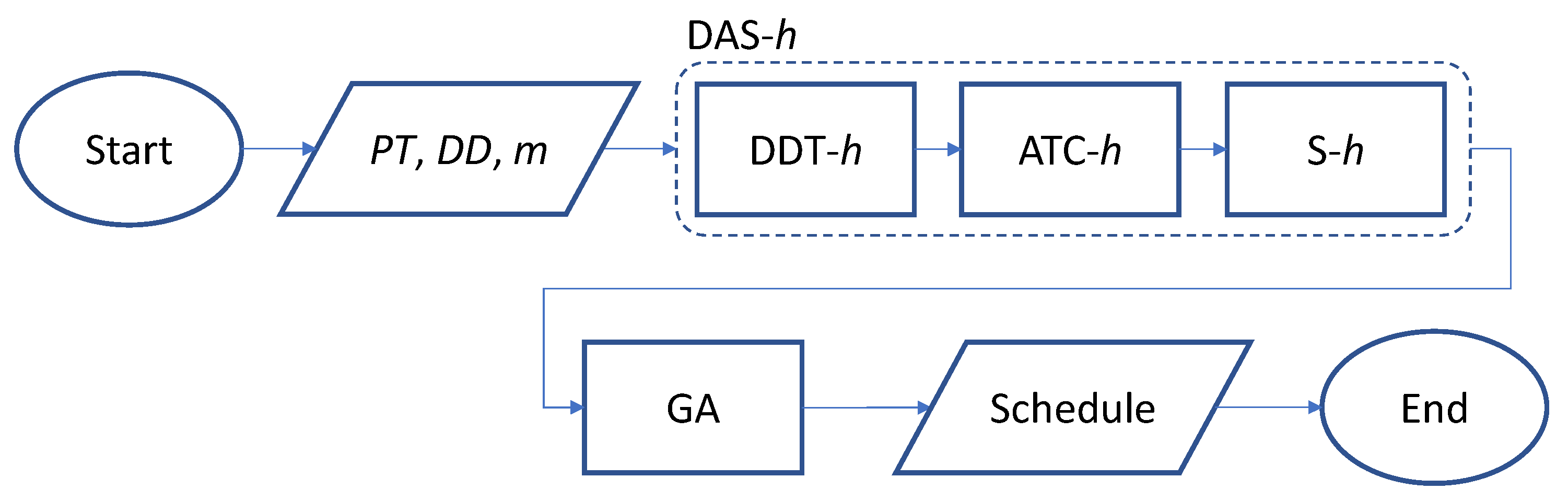
2. The Framework of the Proposed Heuristic-Guided Genetic Algorithm (DAS/GA)
The meta-heuristic algorithm DAS/GA proposed in this article consists of heuristic DAS-
h, followed by GA. DAS-
h itself consists of 3 heuristics working sequentially: Due Date Tightness heuristic (DDT-
h), Apparent Tardiness Cost heuristics (ATC-
h), and Swap heuristic (S-
h).
Figure 1 shows the flowchart of the proposed DAS/GA.
DAS/GA starts with the construction heuristic (DDT-h), which assigns jobs to different machines based on their due dates’ tightness index values. Then, the produced schedule is fed into the modified version of the ATC heuristic (ATC-h) to further improve the schedule. The produced schedule is fed into a third improvement heuristic (S-h), which will fine-adjust the schedule. The output schedule of S-h is used as one chromosome (i.e., schedule) to seed the initial population in the GA. The heuristics and the GA comprising DAS/GA meta-heuristic are discussed in detail in the following sections.
2.1. Due Date Tightness Heuristic (DDT-h)
In DDT-
h, jobs are assigned to different machines based on their Due Date Tightness index
values. This index is calculated by Equation (1), in which the
and
are the due date and the processing time for job
i, respectively. DDT-
h sorts the jobs in an ascending order based on their
values such that a smaller
value indicates a higher priority job.
To illustrate how the DDT-
h works, consider 2 machines and 10 jobs along with their processing times and due dates, as shown in
Table 1. Their
values were calculated according to Equation (1) and are recorded in
Table 1.
The 10 jobs are sorted in ascending order based on their
values, as reported in
Table 2.
After jobs were sorted, the job with the smallest
value is dispatched as the first job on the first machine, the job with the second-smallest
value is dispatched as the first job on the second machine, the job with third-smallest
value is dispatched as the second job on the first machine, and so on. The resulting schedule is summarized in
Table 3.
2.2. Apparent Tardiness Cost Heuristic (ATC-h)
The Apparent Tardiness Cost heuristic (ATC-
h) is an iterative heuristic that schedules jobs one at a time from a set of remaining available jobs. The heuristic contains a priority index
that changes dynamically with time
. Variations of ATC-
h were explained, among other references, in refs. [
17,
20]. We highlight the main aspects of ATC-
h in this article for convenience and modify it to suit the
problem at hand. The
is calculated by multiplying two terms, which are the Weighted Shortest Processing Time (
) and the Least Slack (LS), as in Equation (2):
The Weighted Shortest Processing Time (
) is given by Equation (3):
and the LS is given by Equation (4):
where
is the cumulative time for predecessor job
k,
is the mean of the processing times for the remaining jobs, and
is a look-ahead parameter, which is determined through experimentation. According to ref. [
17],
can be calculated as in Equation (5):
Substituting Equations (3) and (4) in Equation (2) gives the final equation for
as in Equation (6):
where
is given by Equation (5). It should be noted that the processing time for a job includes its setup time, and the setup time for the job is independent of the sequence that includes the job, as stated in assumption 3 in this article. Hence, the equations reported in ref. [
17], which assume a dependent setup time to derive
, should be modified from their original form in ref. [
17] to Equations (4)–(6).
As seen in Equation (3), is the inverse of the processing times. This means that jobs with lower processing times have higher priority (providing everything else remains the same in ). Moreover, Equation (4) shows that has two possible values: value 1 when the slack value for the job is negative, which indicates that the job is tardy, or any value between 0 and 1 when the slack value is not negative, which indicates that the job is not tardy. This means that a tardy job has the highest possible value and consequently has the highest possible value among the jobs with equal processing times.
Every time a machine is available, the priority indices values of all the remaining jobs are re-calculated, and the job with the highest value is chosen to be processed next. The decision is dynamic, as the value of the job changes over time because it depends on , the cumulative time for its predecessor.
The ATC-
h needs an initial schedule to work on. This matter makes the final schedule for ATC-
h dependent on the initial schedule provided.
Table 4 shows a possible initial schedule for ATC-
h.
Table 5 shows the
values generated for the data in
Table 1 based on the initial schedule provided in
Table 4.
Table 6 shows the schedule produced using ATC-
h.
Figure 2 shows the standardized values of
and
for the 10 jobs described in
Table 1. In ATC-
h, as
value, the Due Date Tightness (DDT), increases, the
value decreases, and consequently the priority of the job decreases, while in DDT-
h, as the DDT value increases, the
value increases but the priority of the job decreases.
The Figure shows that the two heuristics have the same basic behavior for jobs with small values of DDT like jobs 2, 3 and 7 but have fundamentally different behavior for jobs with large values like jobs 4 and 8. This difference in the behavior is because the ATC-h takes into account the cumulative processing time for the predecessor in calculating while DDT-h does not. The effect of the on the values in ATC-h is evident in jobs 2 and 8, where both jobs have very close values even though they have a big difference in their DDT values.
2.3. Swap Heuristic (S-h)
The aim of the Swap Heuristic (S-h) is to fine-adjust the schedule by removing one job (with positive tardiness) at a time from a tardy machine and assigning it to the machine with the lowest total tardiness. This heuristic is a fine-adjusting heuristic, so it is meant to be applied after ATC-h, which is a coarse-adjusting heuristic. The aim of this heuristic is to level the load on the machines. S-h is similar to ATC-h in terms of the need for an initial schedule and in terms of using the cumulative times in their calculations.
The pseudo-code for this heuristic is as follows (Algorithm 1):
| Algorithm 1: The pseudo-code of the Swap Heuristic (S-h) |
|---|
| 1: | Input schedule from ATC-h |
| 2: | Calculate the tardiness for each machine in machine set |
| 3: | Determine the machine with lowest |
| 4: | Determine the set that contains the rest of the other machines such that |
| 5: | Determine the set of jobs on |
| 6: | Calculate |
| 7: | Do WHILE the overall total tardiness is improving or termination condition is reached |
| 8: | FOR all machines indexed in do the following |
| 9: | FOR all jobs indexed in do the following |
| 10: | Calculate the cumulative processing time for job i on |
| 11: | IF do the following |
| 12: | Remove job from and assign it to the end of the schedule for |
| 13: | Update , , ,, and |
| 14: | Go to DO WHILE loop |
| 15: | END IF |
| 16: | END FOR indexed |
| 17: | END FOR indexed |
| 18: | END DO WHILE |
| 19: | Report the new Schedule |
The heuristic chooses the job to be moved according to the Ineq. 7 (Equation (7)).
Ineq. 7 states that moving a tardy job from any machine in to the end of the schedule for always results in an improvement in the overall tardiness of the schedule. The left-hand side of the inequality is a quasi-representation of the new tardiness value for the removed job in the new machine, while the right-hand side is a quasi-representation of the tardiness value for the removed job in its original machine. If the left-hand side is less than the right-hand side of the inequality, then removing job from the current machine and assigning it to guarantees enhancement of the overall total tardiness of the schedule by the difference between the left-hand side and the right-hand side values.
To illustrate the effect of this heuristic, consider the data in
Table 7 and the corresponding proposed schedule in
Table 8.
The total tardiness for machine 1 is 7802 and for machine 2 is 1934; the overall total tardiness for the schedule is 9736. The cumulative processing time for machine 2, which is
in this case, is 2434; hence, feeding the data of job 10 in Ineq. 7 gives a correct inequality, as shown below:
Thus, removing job 10 from machine 1 and assigning it at the end of the schedule for machine 2 should improve the overall total tardiness for the schedule by 2301 − 2285 = 16. In fact, removing job 10 from machine 1 and assigning it at the end of the schedule for machine 2 gives an overall total tardiness of 9720, which is 16 units less than the total tardiness of the original schedule, with total tardiness for machine 1 of 5501 and total tardiness for machine 2 of 4219. It should be noticed here how S-h levels the load on the machines and enhances the overall total tardiness of the schedule.
2.4. Genetic Algorithm (GA)
The GA has been used intensively in PMS with the aim of minimizing the overall total tardiness of the schedule [
25,
33,
34,
35]. GA has two kinds of operations: the genetic operation and the evolution operation. Crossover and mutation in GA belong to the genetic operation, while the selection mechanism belongs to the evolution operation [
55]. The crossover operator in GA aims to roughly search the solution space while the mutation operator aims to finely search the solution space by exploiting the promising areas found by the crossover operator [
56].
Chromosome representation, mutation, and selection strategies should be tailored to fit the problem at hand. These strategies are explained in the following sections.
2.4.1. Chromosome Representation
In this proposed GA, the chromosome consists of rows, one row for each machine, and columns (positions) for each row, to ensure that each machine has at least one job on it. In this representation, gene means that the position on the machine is occupied by job . In this representation, each gene carries three pieces of information: the value of the gene itself represents the job, while the position of the gene, determined by and indices, represents the machine and the position on that machine for the job. This representation ensures the feasibility of the chromosomes and offspring and thus avoids the need for any repair actions.
Consider the data used in
Table 1.
Table 9 shows one possible chromosome for this data. The phenotype can be easily retrieved from the genotype in this representation, as gene
means that job 5 is the second job to be processed on machine 2, while
means that there are no jobs processed in position 7 or beyond for machine 1.
2.4.2. Fitness Function
In this GA, the fitness function used is the overall total tardiness of the schedule, as expressed in Equation (8):
where
,
and
are the start time, processing time, and due date for gene
.
The fitness function value for the chromosome in
Table 9 is as follows:
2.4.3. Mutation
This GA is a crossover-free GA in which only mutation is used to produce the offspring from a single parent. Four different mutation types were used to mutate the selected chromosome. The Two Genes Exchange mutation (TGEm) affects only two jobs on the same machine, as it chooses two random jobs from a randomly selected machine and switches their positions. The Number of Jobs mutation (NoJm) changes the number of jobs on two randomly selected machines as it swaps randomly selected jobs from one randomly selected machine to another randomly selected one, provided that the minimum of one job per machine constraint is conserved. NoJm imitates the S-h, but it differs from S-h in two aspects. First, S-h swaps one job each time it is applied while NoJm may swap more than one job each time it is applied. Second, unlike S-h, NoJm does not guarantee that the change is beneficial. The Flip Ends mutation (FEm) flips the ends of the schedule for a randomly selected machine such that the first job becomes the last job and the last job becomes the first job on that machine. Flip Middle mutation (FMm), flips the sequence of the jobs between two randomly selected positions near the middle of the machine’s schedule.
TGEm plays the role of the traditional mutation in the GA, in which it generates a limited disturbance in the chromosome; hence, it performs fine search. The other three types of mutations play the role of crossover in the GA, as they introduce high disturbances in the chromosome; hence, they play the role of coarse search. The offspring produced by these four types of mutations are always feasible offspring thanks to the chromosome representation discussed earlier. Consequently, there is no need for any repair actions on the offspring. Moreover, in this GA, a 25% mutation rate is adopted. This means that the number of offspring generated by mutation is the same as the population size, as each chromosome selected for the mutation will produce 4 offspring.
2.4.4. Selection
An elitist selection strategy is adopted in this GA. Under this strategy, all the parents and the offspring form a pool in which they have to compete for their survival. Those who have better fitness values will be selected as the parents of the next generation.
2.5. Mathematical Model
Binary programming for
is formulated in studies such as refs. [
57,
58]. The objective function of this model is
In this mathematical model, indices , and are indices for job, position, and machine, respectively, and is the number of positions on the machine. Moreover, if job is processed in position at machine and is “0” otherwise, is the completion time for position j at machine , is a positive value that represents the tardiness value for position at machine .
Equation (9) calculates the overall total tardiness of the schedule by summing the individual tardiness values for the positions on the machines. Equation (10) guarantees that each job is assigned only once, while Equation (11) guarantees that each position on each machine, if occupied, will be occupied only once. Equation (12) calculates the cumulative processing time for the job, and Equations (13) and (14) together dictate that if the position on the machine is occupied by a tardy job, then the tardiness of the position equals the tardiness of that job; otherwise, the tardiness of the position and consequently the tardiness of the job is zero.
3. Performance Measures
The performance of DAS-
h, DAS/GA, and GA was measured in this article using two performance measures suggested by ref. [
17], (Relative Error (
) and Average Relative Improvement (
)), and a third performance measure that is suggested in this article: the standardized overall total tardiness
.
is the difference between the tardiness of the method used
and the tardiness of the optimal schedule
found by the binary programming model discussed in
Section 2.5 using CPLEX software relative to
. Mathematically
is given by Equation (16). It should be noted that this measure can only be used when
. If
could not be found due the memory limitations or if
,
will be substituted by
which is the best
found among the different methods used to solve the problem.
is used only with GA and DAS/GA to measure their tardiness
with respect to the tardiness of DAS-
h, which is
. Mathematically, ARI is given by Equation (17):
is the relative deviation between the overall total tardiness of the method and the minimum overall total tardiness among the methods used, divided by the overall total tardiness among the methods used. Mathematically,
is given by Equation (18):
It should be noted that and is the same for cases where .
5. Results and Experiments
Table 10 shows the performance measures for 18 problems generated according to Fisher’s standard method as discussed earlier. It should be noted that CPLEX software did not find the optimal solution, Opt.
for problems beyond problem 11 due to memory limitations. This shows the importance of this work and other related works in solving big NP-hard PMS problems where binary programming fails due to technical issues.
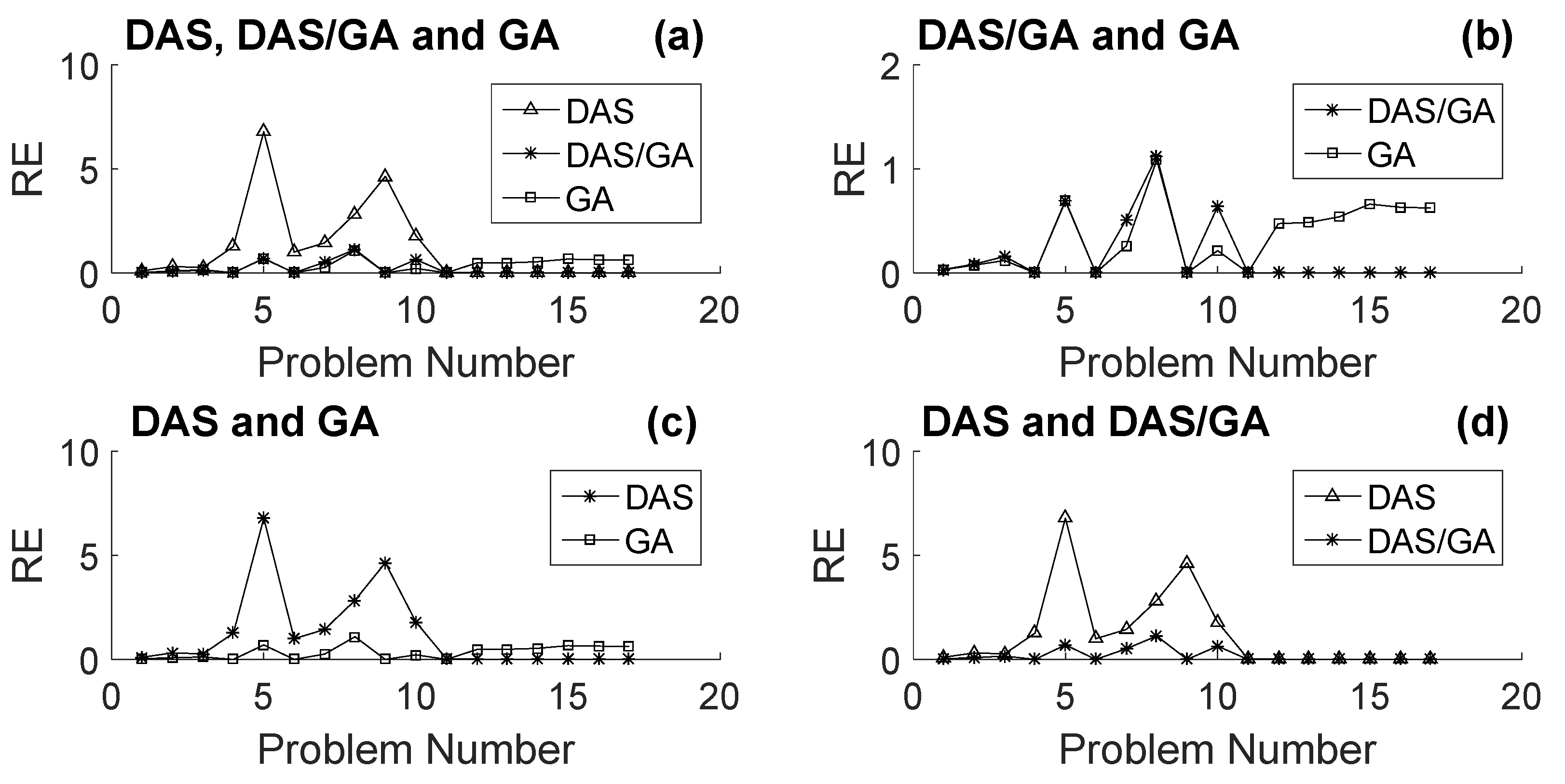
Figure 3a shows a comparison between the performances of the different methods using the
measure.
Figure 3b shows that the performance of GA slightly outperformed the performance of DAS/GA for small problems and significantly for medium problems. On the other hand, for large problems, the performance of DAS/GA significantly outperformed the performance of GA. This means that DAS-
h helped GA improve its performance significantly in large problems but deteriorated its performance for medium problems.
Figure 3c shows that the trend between the performances of GA and DAS-
h is the same as the trend captured in
Figure 4b between GA and DAS/GA. The performance of GA slightly outperformed the performance of DAS-
h for small problems and significantly for medium problems, while for large problems the performance of DAS-
h significantly outperformed the performance of GA. From
Figure 3b,c, one can see that the behavior of DAS-
h masks the behavior of DAS/GA for large problems, as DAS/GA has the same behavior of DAS-
h relative to GA in this range of problem sizes. The comparison between the performance of DAS-
h and DAS/GA shown in
Figure 3d supports this argument. The Figure shows that DAS/GA slightly outperformed DAS-
h for small problems and significantly for medium problems; the methods had a negligible difference in their performance for large problems.
The negligible difference in performance between DAS-
h and DAS/GA shown in
Figure 3d for large problems suggests that when combining DAS-
h with GA to form the DAS/GA meta-heuristic, DAS/GA will be trapped in a region of good local optima created by DAS-
h; consequently, the effect of GA will be negligible as it is trapped in this region.
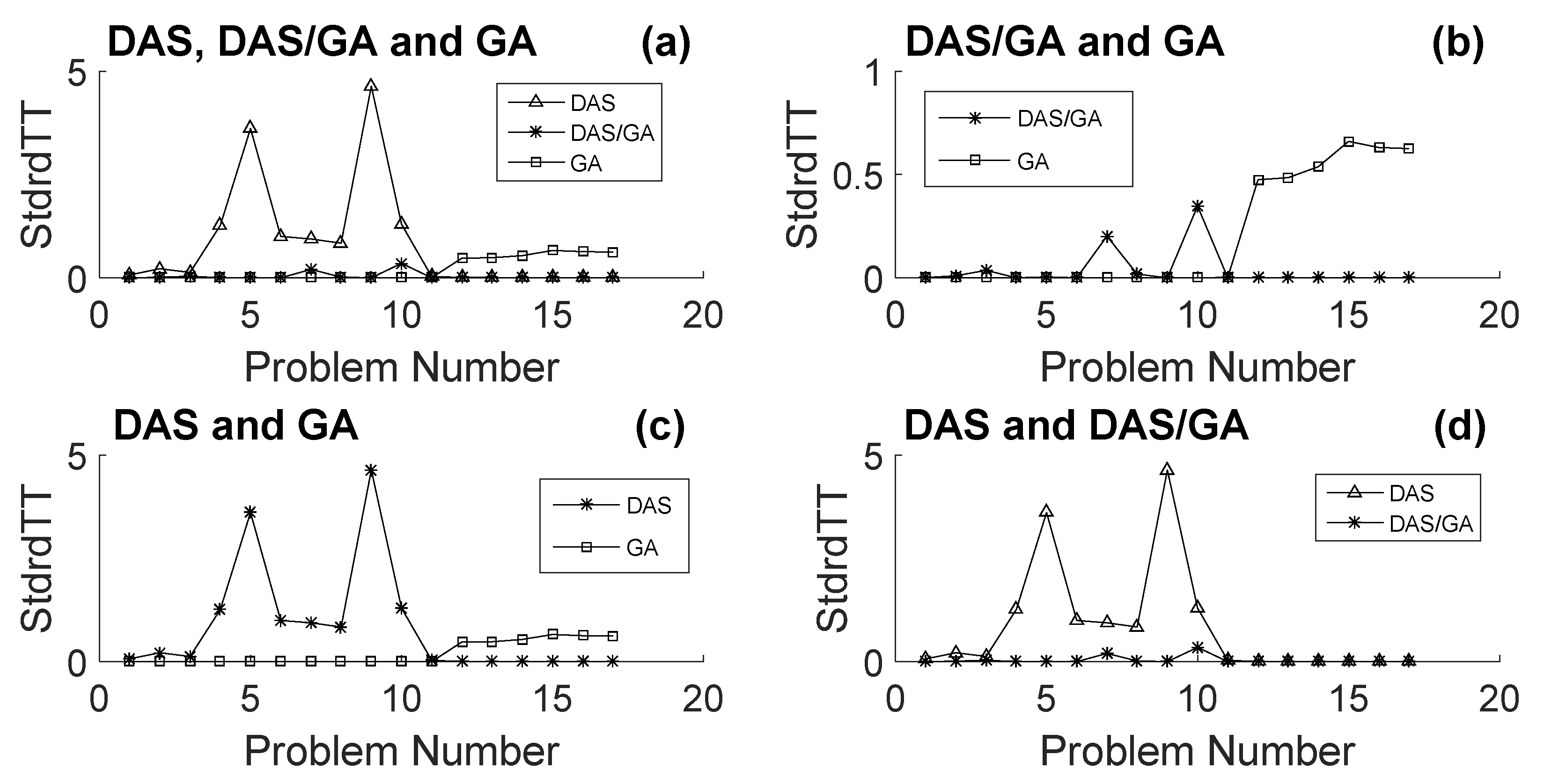
In
Figure 4, the standardized total tardiness values
for the different methods were compared.
Figure 4a shows the exact same trends as found in
Figure 3a between the performances of the different methods but using the
performance measure.
Figure 4b shows that GA slightly outperformed DAS/GA for small problems and significantly for medium problems. For large problems, DAS/GA significantly outperformed GA, which is the same as the trend in
Figure 3b.
Figure 4c shows the same trend found in
Figure 3c between the performances of GA and DAS-
h.
Figure 4d shows that DAS/GA outperformed DAS-
h for small problems and significantly for medium problems; however, the methods had a negligible difference in their performance for large problems, which is the same trend as found in
Figure 4d.
Figure 5 shows a comparison between DAS/GA and GA using
measure. The figure reveals the same trend found earlier using
and
measures in
Figure 3b and
Figure 4b, respectively: GA slightly outperformed DAS/GA for small problems and especially for medium problems. For large problems, DAS/GA significantly outperformed GA. DAS-
h helped GA to improve its performance significantly in large problems but deteriorated its performance for small and especially for medium problems, as the
values for DAS/GA for large problems are almost constant and approximately 1, but for small problems and especially for medium problems, the values are less than 1.
Moreover, looking at the values for DAS/GA for large problems supports the argument made earlier: DAS-h creates a region of good local optima for large size problems that trap GA in it and renders the effect of GA negligible, and hence in this region DAS-h dictates the behavior of DAS/GA. The values of support this argument, as the values for large problems are almost 1, which indicates that the behavior of DAS/GA is very close to the behavior of DAS-h, and hence the effect of GA is almost negligible in DAS/GA compared to the effect of DAS-h.
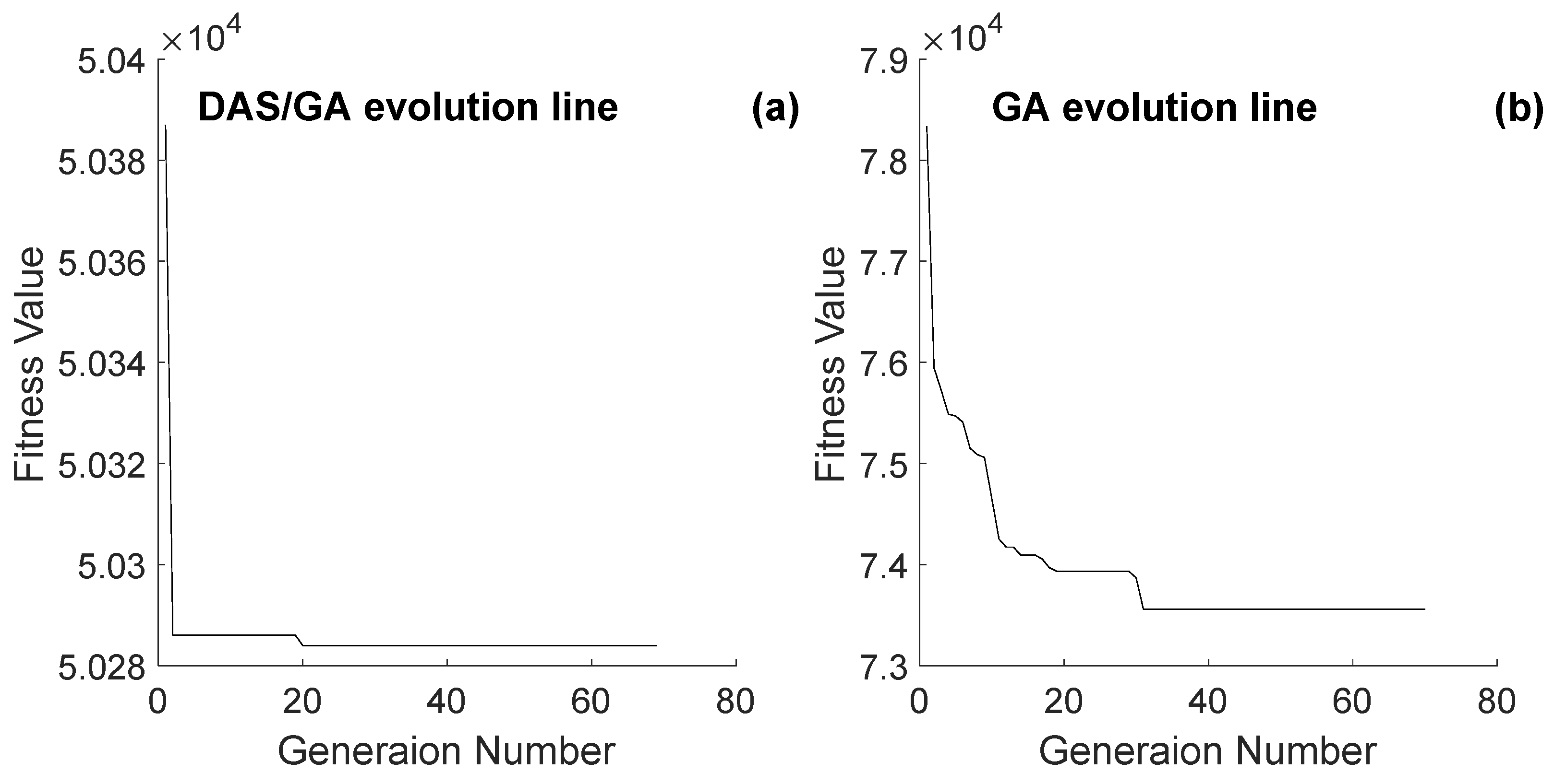
Figure 6 compares the evolution line of DAS/GA and GA for problem 500_10_05_05. The Figure shows the same basic behavior for their evolution lines, except that DAS/GA’s evolution line, shown in
Figure 6b, started from a better point and reached a better fitness value than GA. Moreover, the figure shows that GA had a higher number of enhancement points in its evolution line than DAS/GA. This observation agrees with what was noted earlier about the effect of the region of local optima that DAS-
h introduces in DAS/GA.
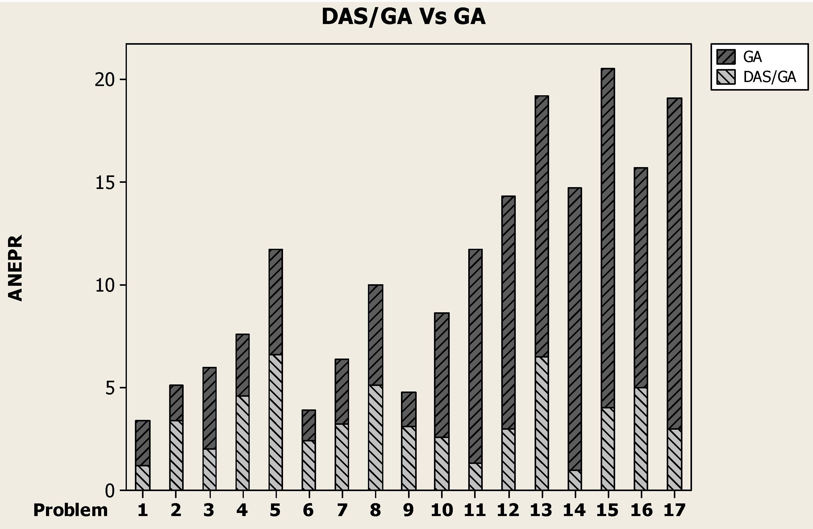
To explore this observation more,
Figure 7 shows a comparison between Average Number of Enhancements Per Replicate (ANEPR) for both meta-heuristics DAS/GA and GA. It is noted that as the problem size increased, the ANEPR for the GA method increased significantly, while for the DAS/GA method, the ANEPR was independent of the problem size, as the DAS/GA method showed a random relation between ANEPR and the problem size.
This shows that generating a strong initial solution for DAS/GA for large-size problems using DAS-
h will cause DAS/GA to be trapped in a region of local optima and hence limit the number of enhancements made to the strong initial solution. This matter makes the difference between the performances of DAS-
h and DAS/GA negligible, as revealed in
Figure 3d and
Figure 4d and the DAS/GA curve in
Figure 5, and hence supports the argument made earlier that DAS-
h dictates the behavior of DAS/GA in this region of large-size problems.
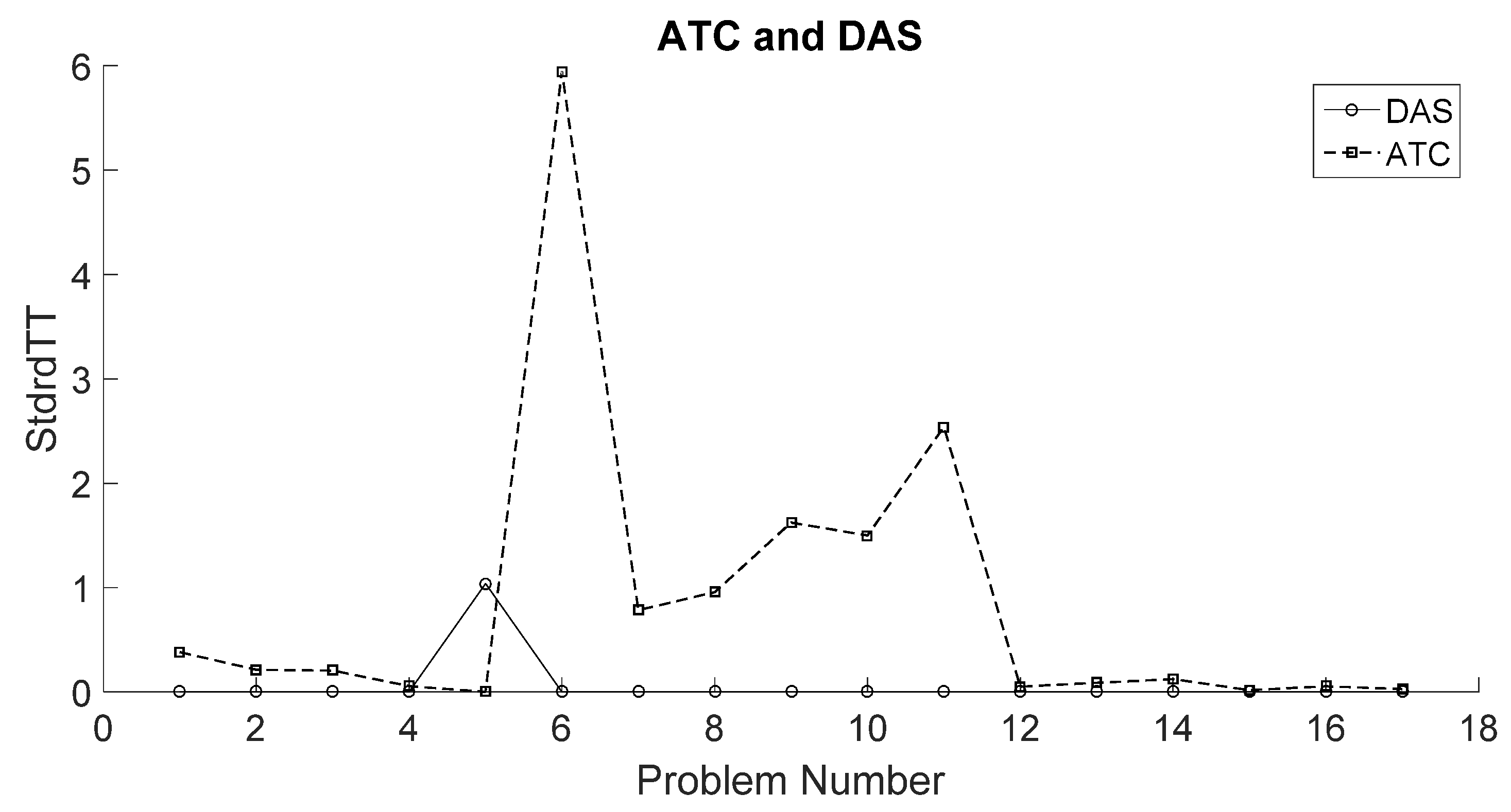
Figure 8 shows a comparison between the performance of ATC-
h and DAS-
h. The Figure shows that DAS-
h outperformed ATC-
h for most of the problems, whether they are small, medium, or large. Moreover, the Figure shows that the largest difference between the two heuristics is for the medium-size problems, where DAS-
h significantly outperformed ATC-
h.
This superior performance of DAS-h can be linked to the structure of this heuristic, where DDT-h first constructs a good initial feasible schedule; then, this schedule is coarse-tuned using ATC-h, after which the S-h fine-tunes the schedule.
This superior performance of DAS-h in medium-range problems explains the strong deterioration in the performance of DAS/GA relative to GA in medium-size problems. DAS-h generates a region of local optima that traps DAS/GA, and consequently the performance of DAS/GA is limited in this region to the performance of DAS-h. Unlike the case with large-size problems, in medium-size problems GA alone can reach better regions than the region provided by DAS-h in DAS/GA; therefore, GA alone outperforms the performance of DAS/GA in medium-size problems, as the region provided by DAS-h traps DAS/GA in it and limits the capabilities of GA in DAS/GA to reach better regions.


