Acetone–Butanol–Ethanol Fermentation Phenomenological Models for Process Studies: Parameter Estimation and Multi-Response Model Reduction with Statistical Analysis

Abstract

A phenomenological multi-response multi-parameter Acetone–Butanol–Ethanol fermentation dynamic model is developed and calibrated for fermentation process studies. The model was constructed based on other models reported in the literature and was calibrated with a maximum likelihood parameter estimation over Acetone–Butanol–Ethanol fermentation experimental data from the literature. After parameter estimation, a rigorous statistical analysis was conducted to evaluate standard deviations of estimated parameters and predicted responses as well as their respective 95% probability confidence intervals for correct parameters and responses. The significance of parameters was assessed via a Fisher’s F test. From the Base-Model with 17 parameters, a tight, more compact, Reduced-Model was developed with 9 highly significant parameters after deleting 8 nonsignificant parameters from the Base-Model and re-estimating the remaining 9 parameters. This Reduced-Model showed good adherence to the experimental data and had better performance comparatively relative to the Base-Model with 17 parameters using two different inhibition functions reported in the literature. The Reduced-Model is sufficiently good for preliminary engineering and economic assessments of ABE fermentation processes.

1. Introduction

Acetone–Butanol–Ethanol (ABE) fermentation gets its name due to the simultaneous production of acetone, butanol, and ethanol by Clostridium sp. bacteria over sucrose substrates. This process was used in industrial scales at the beginning of the 20th century due to the high acetone demand for the production of cordite, which was used as an alternative for gunpowder during World War I [1]. At this time, the first ABE fermentation patent was filed by Charles Weizmann [2].

However, in the decade of the 1950s, new petrochemical processes for Butanol and Acetone productions initiated operations around the world, with incredible low-cost performance and high efficiency thanks to low-cost utilities and low-cost raw materials from the petroleum industry, which experienced a boom at that time. The immediate consequence was that ABE fermentation lost its importance and became practically economically unfeasible due to the high competitiveness of petroleum and petrochemical industries. As a result, until the middle of the 1980s, there were no important industries in the world using ABE fermentation for the production of n-butanol [1]. In parallel, studies on ABE fermentation were also almost abandoned and reinitiated only in the 1980s due to high oil prices that started with the Oil Crisis in the preceding decade. However, the Oil Crisis did not stop in the 1970s and indeed became a chronical and cyclic event throughout the incoming decades until today. Consequently, the continued Oil Crisis raised the prices of petroleum and petrochemical commodities, deflagrating a research boom on alternative fermentative routes for the production of fuel and chemical commodities. This gives rise to several large-scale successful industrial fermentation routes around the world, such as the bioethanol industry from sugarcane in Brazil, which is currently the first in importance in the world. In a similar manner, ABE fermentation research experienced a rebirth in the 1980s. Mulchandani and Volesky (1986) [3] was one of the high-quality studies on ABE fermentation of the 1980s. Among other things, this study presented a large set of high-quality multi-response experimental points on dynamic ABE fermentation and also developed a successful dynamic multi-response model for this fermentation.

In addition, about 20 years ago, the interest on sustainable processes that are not dependent on fossil fuels such as carbon raw materials started growing due to a different factor, namely, climate change concerns. In other words, the development and study of technologies based on renewable raw materials for chemical and biofuel production increased substantially once more. In concordance with this trend, the interest for ABE fermentation renewed, and several studies have been conducted, aiming to improve ABE fermentation’s economic competitiveness against the fossil-based petrochemical route [4].

The main challenge for the economic feasibility of ABE fermentation is the toxicity of metabolites produced by the microorganism itself, primarily butanol. This toxicity inhibits microorganism growth and results in low ABE titers that are not higher than 20 g/L [1]. Yang and Tsao (1994) [5] showed, by using an experiment design, that not only butanol but also acetic and butyric acids inhibit Clostridium sp.’s growth. However, authors such as Rochón et al. (2017) [6] do not consider such inhibitions in their mathematical modeling, raising the question of whether this acid inhibition is prevalent or not.

There are two main approaches researchers follow to solve this problem. The first approach uses synthetic biology, using concepts such as the metabolic adaptation and genetic engineering of butanol-producing bacteria to improve their tolerance to inhibitory substances. Jiang et al. (2009) [7] engineered a Clostridium acetobutylicum to decrease the effects of acetone-producing genes in order to increase final butanol titers and productivity. The study resulted in a butanol yield improvement from 57% to 70.8%. Jiménez-Bonilla et al. (2020) [8] overexpressed efflux pump genes from Pseudomonas putida on Clostridium saccharoperbutylacetonicum in order to enhance the tolerance to lignocellulosic-biomass-derived inhibitors for bio-butanol production. Even though butanol productivity was not changed, the engineered strain was capable of growing in media containing notable inhibition compounds such as furfural and ferulic acid, making way for the utilization of lignocellulosic raw materials for the production of butanol. The second approach seeks to improve butanol productivity via alternative process schemes and alternative raw materials without changing microorganism. Some authors tested alternative raw materials such as black strap molasses and spent coffee grounds to produce biobutanol via ABE fermentation [9,10]. Saadatinavaz et al. (2021) [11] applied a hydrothermal pretreatment to orange waste to produce biobutanol, biohydrogen, and biomethane, achieving yields as high as 42.3 kg butanol per 1000 kg of orange waste. In terms of process configuration, some studies mainly attempt to remove butanol from the fermentation broth while growth is still happening in order to decrease inhibition and to enhance butanol productivity. This is often called in situ butanol recovery. Setlhaku et al. (2013) [12] investigated gas stripping and per-evaporation techniques to remove butanol from the media. Gas stripping was able to achieve butanol concentrations up to 59 g/L, while per-evaporation produced permeates with 167 g/L of butanol. Valles et al. (2021) [13] applied gas stripping as an in situ product recovery process to simultaneous saccharification and fermentation fed-batch processes. The authors were able to increase butanol productivity by 100% when compared with the same process without product recovery.

1.1. n-Butanol: Applications and Market

n-Butanol is a four-carbon saturated linear alcohol mainly used for the production of acetates and acrylates. Its world market value is estimated at USD 3.1 billion in 2020, and it is projected to reach USD 4.0 billion by 2025 [14]. It is mostly used as a secondary chemical to produce derivatives, such as acetates, acrylates, glycolic ethers, and butylic esters. These derivatives are used, primarily, for cosmetics, shampoos, detergents, and soaps and to improve fragrances and perfumes [14]. As a biofuel in fuel blends, n-butanol can be used in current vehicle engines; it has a high energy density and increases the tolerance to water contamination [15]. As an additive, when n-butanol is mixed to another fuel used in internal combustion engines, it only generates carbon dioxide, making it an environment friendly biofuel. Compared to ethanol, it has higher heat capacities, lower vapor pressure, and is less volatile and less corrosive [16].

1.2. ABE Fermentation Mathematical Modeling

ABE fermentation has been modeled since the 1980s. The developed models range from simple fermentation stoichiometric equations [17] to complex kinetics equations based on microorganism metabolic routes. Older models represented the ABE fermentation process in a macroscopic manner, associating the quantity of the consumed substrate to generated biomasses and metabolites, as is the case with the model from Mulchandani and Volesky (1986) [3]. Newer models aim to quantify metabolic fluxes, looking for intracellular production bottlenecks and the optimization of substrate utilization as in the models of Shinto et al. (2007) [18] and Buehler and Mesbah (2016) [19]. Even though the necessity of modeling metabolic fluxes is clear and valuable for understanding cell mechanisms, the pragmatic approach based on older models is more useful on practical grounds for process engineering, as it simplifies calculations and process simulations for cost-estimation purposes and techno-economic feasibility studies.

The effect of the inhibition on the microorganism growth rate still poses a modeling challenge. Inhibition is often represented as an additional factor relative to the microorganism specific growth-rate term, as shown in Equation (1), where the inhibition term $f\left(I\right)$ can be expressed in various ways, as shown in Table 1.

$$\mu ={\mu }_{max}\frac{S}{K_S+S}f\left(I\right)$$

(1)

For the most part, authors often develop models to represent their experiments in order to assess which variable impacts more on productivity to optimize their processing unit or to assess the impact of one variable on another. These models are usually tied to the design of experiments and ANOVA analysis in order to judge the significance of the model and their parameters. Many studies have been recently reported in the literature with this type of approach [20,21,22].

Table 1. Inhibition terms reported in the literature for ABE fermentation.

Reference	Inhibition Term
Mulchandani & Volesky (1986) [3]	$f\left(I\right)=\{\begin{array}{c}\mathit{exp}\left[-0.01\left(B+BA\right)\right],(B+BA)<8.0 \mathrm{g}/\mathrm{L}\\ 2.16-0.153\left(B+BA\right),8.0\le \left(B+BA\right)\le 13.9 \mathrm{g}/\mathrm{L}\end{array}$
Yang and Tsao (1994) [5]	$f\left(I\right)=1-{\left(\frac{AA}{C_{maa}}\right)}^{maa}-{\left(\frac{BA}{C_{mba}}\right)}^{mba}-{\left(\frac{B}{C_{mb}}\right)}^{mb}-m_1{\left(\frac{AA}{C_{maa}}\right)}^{maa}{\left(\frac{B}{C_{mb}}\right)}^{mb}-m_2{\left(\frac{BA}{C_{mba}}\right)}^{mba}{\left(\frac{B}{C_{mb}}\right)}^{mb}$
Velázquez-Sánchez and Aguilar-López (2019) [23]	$f\left(I\right)=\left(1-\frac{B}{K_P}\right)$
Eom et al. (2015) [24]	$f\left(I\right)={\left(1-\frac{B}{K_B}\right)}^{i_B}{\left(1-\frac{X}{K_X}\right)}^{i_X}$
Buehler and Mesbah (2016) [19]	$f\left(I\right)=\left(\frac{1}{1+\frac{B}{K_B}}\right)\left(1-{\left(\frac{BA}{B{A}_{mas}}\right)}^{mba}\right)\left(1-m_{pH}\left(5.6-pH\right)\right)$
Rochón et al. (2017) [6]	$f\left(I\right)={\left(1-\frac{B}{K_P}\right)}^a$

Table 1. Inhibition terms reported in the literature for ABE fermentation.

Reference	Inhibition Term
Mulchandani & Volesky (1986) [3]	$f\left(I\right)=\{\begin{array}{c}\mathit{exp}\left[-0.01\left(B+BA\right)\right],(B+BA)<8.0 \mathrm{g}/\mathrm{L}\\ 2.16-0.153\left(B+BA\right),8.0\le \left(B+BA\right)\le 13.9 \mathrm{g}/\mathrm{L}\end{array}$
Yang and Tsao (1994) [5]	$f\left(I\right)=1-{\left(\frac{AA}{C_{maa}}\right)}^{maa}-{\left(\frac{BA}{C_{mba}}\right)}^{mba}-{\left(\frac{B}{C_{mb}}\right)}^{mb}-m_1{\left(\frac{AA}{C_{maa}}\right)}^{maa}{\left(\frac{B}{C_{mb}}\right)}^{mb}-m_2{\left(\frac{BA}{C_{mba}}\right)}^{mba}{\left(\frac{B}{C_{mb}}\right)}^{mb}$
Velázquez-Sánchez and Aguilar-López (2019) [23]	$f\left(I\right)=\left(1-\frac{B}{K_P}\right)$
Eom et al. (2015) [24]	$f\left(I\right)={\left(1-\frac{B}{K_B}\right)}^{i_B}{\left(1-\frac{X}{K_X}\right)}^{i_X}$
Buehler and Mesbah (2016) [19]	$f\left(I\right)=\left(\frac{1}{1+\frac{B}{K_B}}\right)\left(1-{\left(\frac{BA}{B{A}_{mas}}\right)}^{mba}\right)\left(1-m_{pH}\left(5.6-pH\right)\right)$
Rochón et al. (2017) [6]	$f\left(I\right)={\left(1-\frac{B}{K_P}\right)}^a$

Specifically, for ABE fermentation, Gattermayr et al. (2021) [25] used an experimental design and model to find out that substrates (glucose) must not be limited and butyric acid should be supplied at a rate of 7.5 mmol.L⁻¹·h⁻¹ in order to maximize its specific butanol production. Recent studies also used phenomenological models to represent their fermentations, although proper statistical analyses were not conducted to assess estimated parameters and responses [26,27].

1.3. The Present Work

With the increasing growth of biotechnology and fermentation processes at the industrial scale, there is an increasing need of techno-economic feasibility analysis to advance different grounds imposed by engineering projects. Being able to calculate and predict mass/energy balances by using mathematical modeling and process simulations is vital for performing such assessments. This entails the need of consistent phenomenological multi-response models that reliably reproduce dynamic or steady-state fermentation processes. Since these are semi-empirical models, they have to be calibrated with reliable experimental data from the literature. To accomplish this, a statistically sound estimation procedure must be followed.

A complete statistical analysis for model’s calibration regarding multi-response ABE fermentation does not exist in the literature. To fill this gap, the present work develops a sufficiently comprehensive multi-response ABE dynamic model and calibrates it according to rigorous statistical procedures over multi-response ABE fermentation dynamic data from the literature. The approach is based on the multi-response Maximum Likelihood Principle and prescribes several rounds of parameter estimation and subsequent parameter elimination by using significance tests in order to reach a tight Reduced-Model with all parameters being sufficiently significant. The achieved multi-response Reduced-Model can reproduce, with sufficient accuracy, ABE fermentations in both dynamic and in steady-state modes. This model is able to support the preliminary techno-economic feasibility analysis of the ABE fermentation process as a whole.

2. Methods

Aiming at to implement an ABE fermentation kinetic model on a computational simulation environment for technology assessment, it is important that the model is based on a species that already has pure properties and binary interaction parameters incorporated in the professional process simulator in question. Because of this, the utilization of more structured fermentation models that consider complex metabolites, coenzymes, and complex reaction pathways is not easy (or even possible) to implement in professional process simulators. In this regard, non-structured models have become more attractive. In consequence, this study will develop an ABE fermentation model based on the non-structured model of Mulchandani and Volesky (1986) [3] here referred to as the MV-Model.

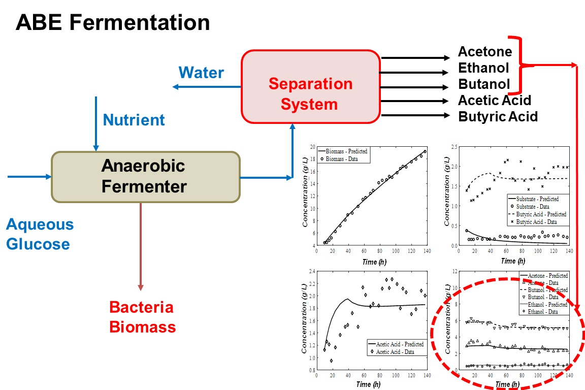
2.1. ABE Fermentation Model Description

An ABE fermentation model is developed based on the Mulchandani and Volesky (1986) [3] model, which represents a continuous ABE fermentation process with cell retention. To formulate it, the following assumptions are adopted:

(1)

The carbon source is the only limiting substrate;

(2)

There is no limitation of nitrogen and nutrients;

(3)

There is product inhibition;

(4)

Acetic acid and butyric acid are reduced to acetone and butanol, respectively;

(5)

Acetone and butanol are also produced directly from carbon substrates;

(6)

Ethanol is produced from carbon substrates only;

(7)

Fermentation is performed at 37 °C and a pH of 4.5 under anaerobic conditions;

(8)

All cells are considered metabolically active and viable.

The microbial growth rate is based on the classical Monod Equation [28] with the addition of inhibition term $f(I)$, as seen in Equations (2) and (3). This term takes into account the growth inhibition by the presence of butanol and/or butyric acid, modeled as an exponential equation when the concentration sum is below 8.0 g/L and by a linear equation when this sum is between 8.0 and 13.9 g/L. According to the authors, this approach encompasses all inhibition ranges from the metabolites, where B and BA represent butanol and butyric acid concentrations in g/L, respectively. Therefore, the biomass generation rate is represented by Equation (3), where ${\mu }_{\max }$ is the maximum growth rate, $K_S$ is the substrate’s affinity constant, and S is the substrate’s concentration (g/L).

$$f(I)=\{\begin{array}{c}\mathit{exp}\left(-0.01(B+BA)\right), (B+BA)<8.0 \mathrm{g}/\mathrm{L}\\ 2.16-0.153(B+BA), 8.0\le (B+BA)\le 13.9 \mathrm{g}/\mathrm{L}\end{array}$$

(2)

$$r_x=\frac{{\mu }_{\max }S.X.f(I)}{K_S+S}$$

(3)

The substrate’s consumption rate is modeled according to Pirt (1975) [29]. In addition, acid reduction to alcohol demands energy, which is obtained by substrate consumption. Therefore, consumption and energy generation terms were added to Equation (4), where $k_1$ and $k_2$ are kinetic constants and $K_{BA}$ and $K_{AA}$ are butyric acid and acetic acid saturation constants, respectively.

$$-r_S=\left(\frac{1}{Y_{X/S}}\mu +m+\left(\frac{S}{K_S+S}\right)\left(\frac{k_{1}BA}{K_{BA}+BA}+\frac{k_{2}AA}{K_{AA}+AA}\right)\right)X$$

(4)

The net butyric acid production rate is the difference between its production and consumption rates in Equation (5), wherein the first term ($r_{BA,P}$) represents the acid production rate calculated by using its yield coefficient in Equation (6), where $Y_{BA/S}$ is the butyric acid yield coefficient, $Y_{X/S}$ is cell yield coefficient, $m$ is cell maintenance coefficient, and $X$ is the biomass concentration (g/L). The butyric acid consumption rate is written as a function of acid and substrate concentrations. These functions are similar to the Langmuir adsorption isotherm and represent the adsorption of butyric acid on the cell wall, as shown in Equation (7). By arranging Equations (6) and (7), Equation (8) gives the net butyric acid consumption rate, where $k_6$ is a fitting parameter.

$$r_{BA}=r_{BA,P}-r_{BA,C}$$

(5)

$$r_{BA,P}=Y_{BA,P}(-r_S)=\frac{Y_{BA/S}}{Y_{X/S}}{r}_X+Y_{BA/S}mX$$

(6)

$$r_{BA,C}=\frac{k_{6}BA}{K_{BA}+BA}\left(\frac{S}{K_S+S}\right)X$$

(7)

$$r_{BA}=\left(Y_{BA/S}m+\left(\frac{S}{K_S+S}\right)\left(\frac{Y_{BA/S}}{Y_{X/S}}{\mu }_{\max }f(I)-\frac{k_{6}BA}{K_{BA}+BA}\right)\right)X$$

(8)

For acetic acid, its net production rate ($r_{AA}$) is analogous to the butyric acid production rate and is represented in Equation (9), where $k_9$ is another fitting parameter.

$$r_{AA}=\left(Y_{AA/S}m+\left(\frac{S}{K_S+S}\right)\left(\frac{Y_{AA/S}}{Y_{X/S}}{\mu }_{\max }f(I)-\frac{k_{9}AA}{K_{AA}+AA}\right)\right)X$$

(9)

The butanol production rate is represented by the sum of its production via substrate conversion and via butyric acid conversion, as shown in Equation (10). The first term is expressed in terms of the butanol yield coefficient ($Y_{B/S}$) in Equation (11) and the second term is similar to butyric acid’s conversion in Equation (12), where $k_{14}$ is another fitting parameter. Using Equations (11) and (12) on Equation (10), the butanol net production rate is written in Equation (13).

$$r_B=r_{B,S}+r_{B,BA}$$

(10)

$$r_{B,S}=Y_{B/S}(-r_S)=\frac{Y_{B/S}}{Y_{X/S}}{r}_X+Y_{B/S}mX$$

(11)

$$r_{B,BA}=k_{14}\frac{BA}{K_{BA}+BA}\left(\frac{S}{K_S+S}\right)X$$

(12)

$$r_B=\left(Y_{B/S}m+\left(\frac{S}{K_S+S}\right)\left(\frac{Y_{B/S}}{Y_{X/S}}{\mu }_{\max }f(I)-\frac{k_{14}BA}{K_{BA}+BA}\right)\right)X$$

(13)

The acetone production rate is expressed similarly as the butanol rate in Equation (14), where $k_{15}$ is a fitting parameter.

$$r_A=\left(Y_{A/S}m+\left(\frac{S}{K_S+S}\right)\left(\frac{Y_{A/S}}{Y_{X/S}}{\mu }_{\max }f(I)-\frac{k_{15}AA}{K_{BA}+AA}\right)\right)X$$

(14)

Finally, the ethanol production rate is expressed as a function of the substrate consumption rate using its yield coefficient in Equation (15).

$$r_E=\left(\frac{Y_{E/S}}{Y_{X/S}}{\mu }_{\max }\frac{S}{K_S+S}f(I)+Y_{E/S}m\right)X$$

(15)

With all components production and consumption rates, the ABE fermentation bioreactor dynamics (considering cell retention) is modeled by using Equations (16)–(22), where $D$ is the process dilution rate and $S_0$ is the substrate feed concentration. This ABE fermentation model represented by Equations (16)–(22) is referred as the Base-Model and has 17 adjustable parameters (${\mu }_{max}, k_1, k_2, Y_{X/S}, m, Y_{BA/S}$, $k_6, Y_{B/S}, Y_{AA/S}, k_9, Y_{A/S}, Y_{E/S}$, $k_{14}, k_{15}, K_S, K_{AA}, K_{BA}$). Notice that after parameter estimation and the deletion of nonsignificant parameters and re-estimation, the Base-Model becomes the Reduced-Model, which is far different from the MV-Model of Mulchandani and Volesky (1986) [3] because the MV-Model did not experience such a statistical treatment.

$$\frac{dX(t)}{dt}=r_X$$

(16)

$$\frac{dS(t)}{dt}=D(S_0-S)+r_S$$

(17)

$$\frac{dAA(t)}{dt}=-D.AA+r_{AA}$$

(18)

$$\frac{dBA(t)}{dt}=-D.BA+r_{BA}$$

(19)

$$\frac{dA(t)}{dt}=-D.A+r_A$$

(20)

$$\frac{dB(t)}{dt}=-D.B+r_B$$

(21)

$$\frac{dE(t)}{dt}=-D.E+r_E$$

(22)

2.2. Parameter Estimation

Parameter estimation is conducted via the Maximum Likelihood Principle, which is implemented for non-linear explicit multi-response models with known inputs, which is the ABE fermentation case. The main reference is [30]. Firstly, the symbols have to be defined as follows:

• $y_n$: nth response of the model where n is a response index (n = 1, 2,…, NR);
• NR: Number of model responses; for the ABE fermentation model NR = 7;
• I, k: Experiment indexes (i, k = 1, 2,…, NE);
• NE: Number of experiments; for the ABE fermentation model NE = 27;
• ${\underset{\_}{y}}_i$: NRx1 vector of observed response values for experiment $i$;
• $\underset{\_}{\underset{\_}{y}}$: NRxNE matrix of observed responses for all experiments
   $\underset{\_}{\underset{\_}{y}}=\left[\begin{array}{cccc}{\underset{\_}{y}}_1& {\underset{\_}{y}}_2& \cdots & {\underset{\_}{y}}_{NE}\end{array}\right]$;
• ${\underset{\_}{\eta }}_i$: Unknown NRx1 vector of correct response values for experiment $i$;
• $\underset{\_}{x}$: NIx1 vector of independent (input) variables of the model
   (NI is number of inputs);
• ${\underset{\_}{x}}_i$: Known vector $\underset{\_}{x}$ for experiment $i$;
• $\underset{\_}{\beta }$: Unknown NPx1 vector of correct model parameters;
• ${\underset{\_}{\beta }}^t=\left[{\beta }_0 {\beta }_1\dots {\beta }_q\right]$ ($NP=q+1$);
• $\underset{\_}{\widehat{\beta }}$: NPx1 vector of estimated model parameters;
• ${\underset{\_}{\widehat{y}}}_i$: NRx1 vector of estimated responses for experiment $i$;
• $\underset{\_}{\underset{\_}{\widehat{y}}}$:NRxNE matrix of estimated responses for all experiments
   $\underset{\_}{\underset{\_}{\widehat{y}}}=\left[\begin{array}{cccc}{\underset{\_}{\widehat{y}}}_1& {\underset{\_}{\widehat{y}}}_2& \cdots & {\underset{\_}{\widehat{y}}}_{NE}\end{array}\right]$;
• ${\underset{\_}{\underset{\_}{W}}}_i$: Weight matrix for responses of experiment i; this matrix is related to the inverse of the variance–covariance matrix of responses for experiment i;
• ${\sigma }_{\epsilon }^2$: Unknown fundamental variance of the problem;
• $\underset{\_}{\underset{\_}{Cov}}({\underset{\_}{y}}_i)={\sigma }_{\epsilon }^2{\underset{\_}{\underset{\_}{W}}}_i^{-1}$: NRxNR variance–covariance matrix of responses of experiment i;
• ${\underset{\_}{\underset{\_}{X}}}_i$: NRxNP Jacobian matrix of model responses to parameters $\underset{\_}{\widehat{\beta }}$ for experiment i.

In addition, the following statistical assumptions are imposed:

(1)

The experiments are independent; i.e., data from experiment i are not influenced by other experiments;

(2)

Experimental responses are independent and each one obeys a normal distribution around the correct response value with the variance given by ${\sigma }_{\epsilon }^2{(0.1*y_{n,k})}^2 (n=1\dots NR, k=1\dots NE)$;

(3)

The model is correct; i.e., with the correct parameter vector ($\underset{\_}{\beta }$), the model generates the correct response vector (${\underset{\_}{\eta }}_i$) for experiment i with inputs ${\underset{\_}{x}}_i$.

From Assumption II, the probability density function (PDF) of the vector of responses for the ith experiment ${\underset{\_}{y}}_i$ is provided by Equation (23), which can be inputted as shown in Equation (24).

$$PDF({\underset{\_}{y}}_i)=\frac{1}{{(2\pi )}^{NR/2}\sqrt{\underset{\_}{\underset{\_}{Cov}}({\underset{\_}{y}}_i)}}\mathit{exp}\left\{-\frac{1}{2}{\left({\underset{\_}{y}}_i-{\underset{\_}{\eta }}_i\right)}^t{\left[\underset{\_}{\underset{\_}{Cov}}({\underset{\_}{y}}_i)\right]}^{-1}\left({\underset{\_}{y}}_i-{\underset{\_}{\eta }}_i\right)\right\}$$

(23)

$$PDF({\underset{\_}{y}}_i)=\frac{\sqrt{\left|{\underset{\_}{\underset{\_}{W}}}_i\right|}}{{(2\pi {\sigma }_{\epsilon }^2)}^{NR/2}}\mathit{exp}\left\{-\frac{1}{2{\sigma }_{\epsilon }^2}{\left({\underset{\_}{y}}_i-{\underset{\_}{\eta }}_i\right)}^t{\underset{\_}{\underset{\_}{W}}}_i\left({\underset{\_}{y}}_i-{\underset{\_}{\eta }}_i\right)\right\}$$

(24)

The Likelihood function for the vector of responses of experiment i is obtained by replacing ${\underset{\_}{\eta }}_i$ by ${\underset{\_}{\widehat{y}}}_i$ in Equation (24), leading to Equation (25) [30].

$$L\left({\underset{\_}{y}}_i,\underset{\_}{\widehat{\beta }}\right)=\frac{\sqrt{\left|{\underset{\_}{\underset{\_}{W}}}_i\right|}}{{(2\pi {\sigma }_{\epsilon }^2)}^{NR/2}}\mathit{exp}\left\{-\frac{1}{2{\sigma }_{\epsilon }^2}{\left({\underset{\_}{y}}_i-{\underset{\_}{\widehat{y}}}_i\right)}^t{\underset{\_}{\underset{\_}{W}}}_i\left({\underset{\_}{y}}_i-{\underset{\_}{\widehat{y}}}_i\right)\right\}$$

(25)

With Assumption I, the total Likelihood function for all experiments is given by Equation (26), which is transformed in Equation (27) after logarithms.

$$L\left(\underset{\_}{\underset{\_}{y}},\underset{\_}{\widehat{\beta }}\right)={\displaystyle \prod _{k=1}^{NE} L\left({\underset{\_}{y}}_k,\underset{\_}{\widehat{\beta }}\right)}$$

(26)

$$\mathit{ln}L\left(\underset{\_}{\underset{\_}{y}},\underset{\_}{\widehat{\beta }}\right)=\frac{1}{2}{\displaystyle \sum _{k=1}^{NE} \mathit{ln}\left|{\underset{\_}{\underset{\_}{W}}}_k\right|}-\frac{NR.NE}{2}\mathit{ln}(2\pi {\sigma }_{\epsilon }^2)-\frac{1}{2{\sigma }_{\epsilon }^2}{\displaystyle \sum _{k=1}^{NE} {\left({\underset{\_}{y}}_k-{\underset{\_}{\widehat{y}}}_k\right)}^t{\underset{\_}{\underset{\_}{W}}}_k\left({\underset{\_}{y}}_k-{\underset{\_}{\widehat{y}}}_k\right)}$$

(27)

The estimation of $\underset{\_}{\widehat{\beta }}$ is performed by maximizing the logarithm of the Likelihood function in Equation (27), which corresponds to minimizing the weighted sum of squares in the last term of Equation (27), since the other terms are constant in Equation (27). This is the objective function for minimization in the Maximum Likelihood Principle and is given in Equation (28) [30]. This minimization was conducted in Matlab^® R2016a. To construct the response weight matrices ${\underset{\_}{\underset{\_}{W}}}_k (k=1\dots NE)$, Assumption II and Assumption I are used again alongside $\underset{\_}{\underset{\_}{Cov}}({\underset{\_}{y}}_i)={\sigma }_{\epsilon }^2{\underset{\_}{\underset{\_}{W}}}_i^{-1}$, leading to Equation (29).

$$\Phi =\frac{1}{2}{\displaystyle \sum _{k=1}^{NE} {\left({\underset{\_}{\widehat{y}}}_k-{\underset{\_}{y}}_k\right)}^t{\underset{\_}{\underset{\_}{W}}}_k\left({\underset{\_}{\widehat{y}}}_k-{\underset{\_}{y}}_k\right)}$$

(28)

$${\underset{\_}{\underset{\_}{W}}}_k=\left(\begin{array}{ccc}\raisebox{1ex}{$1$}\!\left/ \!\raisebox{-1ex}{${(0.1y_{1,k})}^2$}\right.& 0& \begin{array}{cc}\dots & 0\end{array}\\ 0& \raisebox{1ex}{$1$}\!\left/ \!\raisebox{-1ex}{${(0.1y_{2,k})}^2$}\right.& \begin{array}{cc}\dots & 0\end{array}\\ \begin{array}{c}⋮\\ 0\end{array}& \begin{array}{c}⋮\\ 0\end{array}& \begin{array}{cc}\ddots & ⋮\\ \dots & \raisebox{1ex}{$1$}\!\left/ \!\raisebox{-1ex}{${(0.1y_{NR,k})}^2$}\right.\end{array}\end{array}\right)$$

(29)

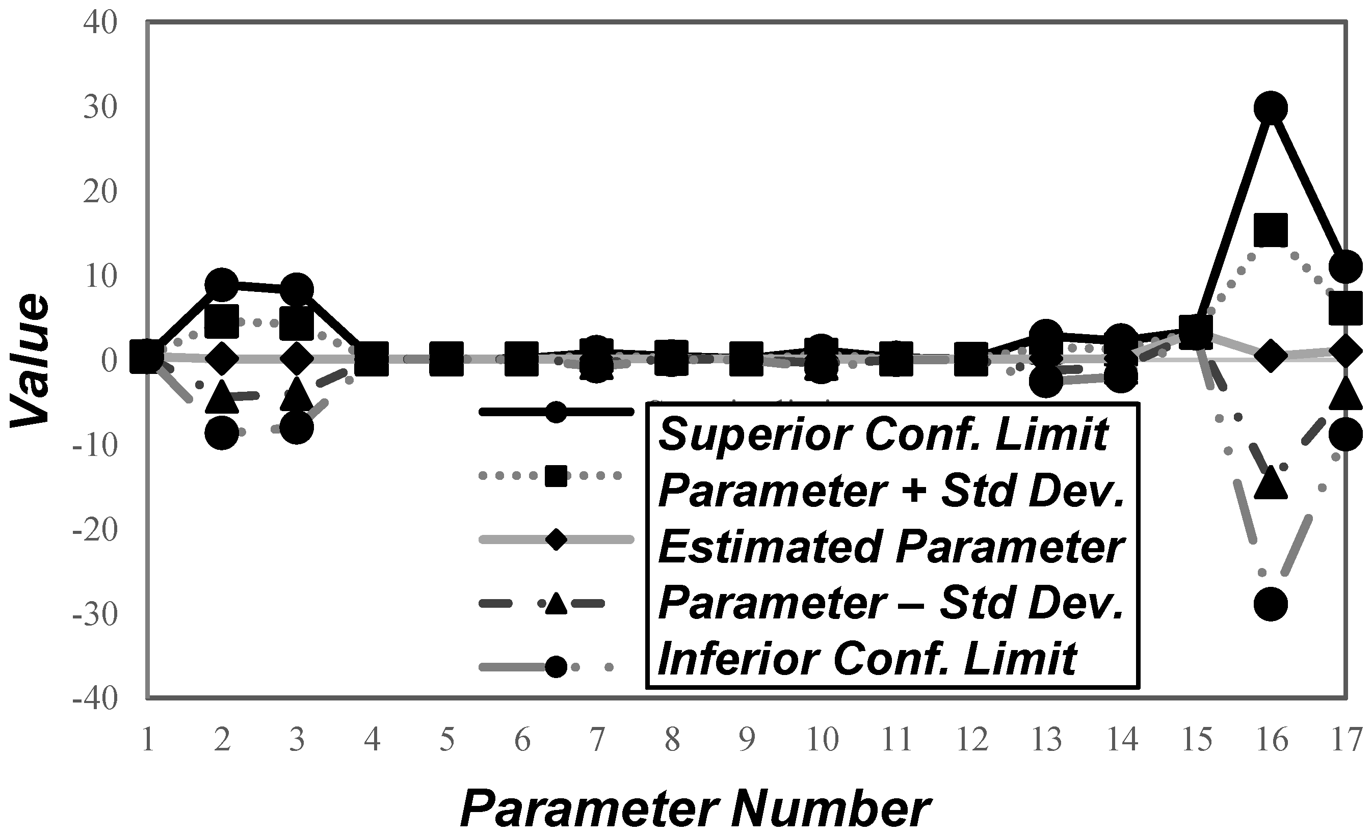
2.3. Statistical Analysis of Estimated Parameters

Statistical analysis has the objective of evaluating the quality of the estimated parameters and estimated responses by means of parameter standard deviations, correct parameter confidence intervals, standard deviations of the estimated responses, and correct response confidence intervals. These calculations are conducted with estimators of the variance–covariance matrix of estimated parameters and estimated responses. All estimators used in this analysis are characterized before utilization.

Admitting that the vector of estimated parameters ($\underset{\_}{\widehat{\beta }}$) is close to the (unknown) vector of correct parameters ($\underset{\_}{\beta }$), a linearization of the predicted response vector of experiment k is constructed in Equation (30). Applying the stationary point condition to the incumbent $\underset{\_}{\widehat{\beta }}$ in Equation (31) and using Equations (28) and (30), one obtains Equation (32). Using Equation (30) in Equation (32), one can write an asymptotic expression for $\underset{\_}{\widehat{\beta }}$ in Equation (33) in order to perform the statistical analysis [30].

$${\underset{\_}{\widehat{y}}}_k\cong {\underset{\_}{\eta }}_k+{\underset{\_}{\underset{\_}{X}}}_k\left(\underset{\_}{\widehat{\beta }}-\underset{\_}{\beta }\right)$$

(30)

$${\underset{\_}{\nabla }}_{\widehat{\beta }}\mathsf{\Phi }=\underset{\_}{0}$$

(31)

$${\displaystyle \sum }_{k=1}^{NE} {\underset{\_}{\underset{\_}{X}}}_k^t{\underset{\_}{\underset{\_}{W}}}_k\left({\underset{\_}{\widehat{y}}}_k-{\underset{\_}{y}}_k\right)=\underset{\_}{0}$$

(32)

$$\underset{\_}{\widehat{\beta }}=\underset{\_}{\beta }+{\left[{\displaystyle \sum }_{k=1}^{NE} {\underset{\_}{\underset{\_}{X}}}_k^t {\underset{\_}{\underset{\_}{W}}}_k {\underset{\_}{\underset{\_}{X}}}_k\right]}^{-1}{\displaystyle \sum }_{k=1}^{NE} {\underset{\_}{\underset{\_}{X}}}_k^t{\underset{\_}{\underset{\_}{W}}}_k\left({\underset{\_}{y}}_k-{\underset{\_}{\eta }}_k\right)$$

(33)

With Equation (33), estimator $\underset{\_}{\widehat{\beta }}$ can be characterized. Since $\underset{\_}{\widehat{\beta }}$ is a linear function of normal vectors $\underset{\_}{y_n}$, $\underset{\_}{\widehat{\beta }}$ also follows a multivariate normal distribution. In addition, since the expected value of responses comprises their correct values in Equation (23), $E\left({\underset{\_}{y}}_k\right)={\underset{\_}{\eta }}_k$, Equation (33) gives $E\left(\underset{\_}{\widehat{\beta }}\right)=\underset{\_}{\beta }$; i.e., $\underset{\_}{\widehat{\beta }}$ is an unbiased estimator, where E(.) is the expectancy operator. Lastly, since experiments are independent by Assumption I, one can write Equation (34). By the definition of the variance–covariance matrix of $\underset{\_}{\widehat{\beta }}$ in Equation (35), Equation (36) is obtained via Equations (33) and (34).

$$E\left\{\left({\underset{\_}{y}}_k-{\underset{\_}{\eta }}_k\right){\left({\underset{\_}{y}}_j-{\underset{\_}{\eta }}_j\right)}^t\right\}=\{\begin{array}{c}\underset{\_}{\underset{\_}{0}},k\ne j\\ {\sigma }_{\epsilon }^2{\underset{\_}{\underset{\_}{W}}}_k^{-1},k=j\end{array} (k, j=1\dots NE)$$

(34)

$$\underset{\_}{\underset{\_}{Cov}}\left(\underset{\_}{\widehat{\beta }}\right)=E\left[\left(\underset{\_}{\widehat{\beta }}-E\left(\underset{\_}{\widehat{\beta }}\right)\right){\left(\underset{\_}{\widehat{\beta }}-E\left(\underset{\_}{\widehat{\beta }}\right)\right)}^t\right]$$

(35)

$$\underset{\_}{\underset{\_}{Cov}}\left(\underset{\_}{\widehat{\beta }}\right)={\sigma }_{\epsilon }^2{\left[{\displaystyle {\displaystyle \sum }_{k=1}^{NE}} {\underset{\_}{\underset{\_}{X}}}_k^t {\underset{\_}{\underset{\_}{W}}}_k {\underset{\_}{\underset{\_}{X}}}_k\right]}^{-1}$$

(36)

Now, when $NE\to \infty$, ${\displaystyle {\displaystyle \sum }_{k=1}^{NE}} {\underset{\_}{\underset{\_}{X}}}_k^t {\underset{\_}{\underset{\_}{W}}}_k {\underset{\_}{\underset{\_}{X}}}_k\to \underset{\_}{\underset{\_}{\infty }}$ and ${\left[{\displaystyle {\displaystyle \sum }_{k=1}^{NE}}\left({\underset{\_}{\underset{\_}{X}}}_k^t {\underset{\_}{\underset{\_}{W}}}_k {\underset{\_}{\underset{\_}{X}}}_k\right)\right]}^{-1}\to \underset{\_}{\underset{\_}{0}}$. Consequently, $NE\to \infty$ implies $\underset{\_}{\underset{\_}{Cov}}\left(\underset{\_}{\widehat{\beta }}\right)\to \underset{\_}{\underset{\_}{0}}$; hence, $\underset{\_}{\widehat{\beta }}$ is also a consistent (coherent) estimator [30].

The characterization of the estimator of predicted responses ${\underset{\_}{\widehat{y}}}_k (k=1\dots NE)$ is analogous to the case of $\underset{\_}{\widehat{\beta }}$. With Equation (30), ${\underset{\_}{\widehat{y}}}_k$ is a linear function of $\underset{\_}{\widehat{\beta }}$ and, therefore, follows a multi-variate normal distribution as well. Moreover, by Equation (30), since $E\left(\underset{\_}{\widehat{\beta }}\right)=\underset{\_}{\beta }$, $E\left({\underset{\_}{\widehat{y}}}_k\right)={\underset{\_}{\eta }}_k$; i.e., estimator ${\underset{\_}{\widehat{y}}}_k$ is also unbiased. Finally, using Equation (30) with the definition of the variance–covariance matrix for ${\underset{\_}{\widehat{y}}}_k$ in Equation (37), Equation (38) is obtained. In a similar manner as used in the previous discussion, when $NE\to \infty$, $\underset{\_}{\underset{\_}{Cov}}\left(\underset{\_}{\widehat{\beta }}\right)\to \underset{\_}{\underset{\_}{0}}$; hence, $\underset{\_}{\underset{\_}{Cov}}\left({\underset{\_}{\widehat{y}}}_k\right)\to \underset{\_}{\underset{\_}{0}}$. Thus, the estimator of predicted responses ${\underset{\_}{\widehat{y}}}_k$ is also consistent (coherent).

$$\underset{\_}{\underset{\_}{Cov}}\left({\underset{\_}{\widehat{y}}}_k\right)=E\left[\left({\underset{\_}{\widehat{y}}}_k-E\left({\underset{\_}{\widehat{y}}}_k\right)\right){\left({\underset{\_}{\widehat{y}}}_k-E\left({\underset{\_}{\widehat{y}}}_k\right)\right)}^t\right]$$

(37)

$$\underset{\_}{\underset{\_}{Cov}}\left({\underset{\_}{\widehat{y}}}_k\right)={\underset{\_}{\underset{\_}{X}}}_k\left(\underset{\_}{\underset{\_}{ Cov}}\left(\underset{\_}{\widehat{\beta }}\right)\right) {\underset{\_}{\underset{\_}{X}}}_k^t$$

(38)

As the variance–covariance matrices of $\underset{\_}{\widehat{\beta }}$ and ${\underset{\_}{\widehat{y}}}_k$ depend on the unknown fundamental variance ${\sigma }_{\epsilon }^2$ via Equation (36), an estimator for ${\sigma }_{\epsilon }^2$ is needed. It can be shown [30] that the best estimator for ${\sigma }_{\epsilon }^2$ is the statistic $S_R^2$, which is the weighted sum of residue squares in Equation (39). With $S_R^2$ in place of ${\sigma }_{\epsilon }^2$, one can write estimators $\underset{\_}{\underset{\_}{C\stackrel{⌢}{o}v}}\left(\underset{\_}{\widehat{\beta }}\right)$ and $\underset{\_}{\underset{\_}{C\stackrel{⌢}{o}v}}\left({\underset{\_}{\widehat{y}}}_k\right)$ for $\widehat{\underset{\_}{\underset{\_}{Cov}}}\left(\underset{\_}{\widehat{\beta }}\right)$ and $\underset{\_}{\underset{\_}{Cov}}\left({\underset{\_}{\widehat{y}}}_k\right)$ in Equations (40) and (41).

$$S_R^2={\widehat{\sigma }}_{\epsilon }^2=\left(\frac{1}{NR.NE-NP}\right){\displaystyle \sum }_{k=1}^{NE} {\left({\underset{\_}{y}}_k-{\underset{\_}{\widehat{y}}}_k\right)}^t{\underset{\_}{\underset{\_}{W}}}_k\left({\underset{\_}{y}}_k-{\underset{\_}{\widehat{y}}}_k\right)$$

(39)

$$\underset{\_}{\underset{\_}{C\stackrel{⌢}{o}v}}\left(\underset{\_}{\widehat{\beta }}\right)=S_R^2{\left[{\displaystyle \sum }_{k=1}^{NE} {\underset{\_}{\underset{\_}{X}}}_k^t {\underset{\_}{\underset{\_}{W}}}_k {\underset{\_}{\underset{\_}{X}}}_k\right]}^{-1}$$

(40)

$$\underset{\_}{\underset{\_}{C\stackrel{⌢}{o}v}}\left({\underset{\_}{\widehat{y}}}_k\right)={\underset{\_}{\underset{\_}{X}}}_k\left(\underset{\_}{\underset{\_}{ C\stackrel{⌢}{o}v}}\left(\underset{\_}{\widehat{\beta }}\right)\right) {\underset{\_}{\underset{\_}{X}}}_k^t$$

(41)

As the diagonal terms of variance–covariance matrices are variances, estimators of standard deviations of estimated parameters and standard deviations of estimated responses are given by square roots of the respective diagonal terms of $\underset{\_}{\underset{\_}{C\stackrel{⌢}{o}v}}\left(\underset{\_}{\widehat{\beta }}\right)$, $\underset{\_}{\underset{\_}{C\stackrel{⌢}{o}v}}\left({\underset{\_}{\widehat{y}}}_k\right)$, as in Equations (42) and (43).

$${\widehat{\sigma }}_{{\widehat{\beta }}_k}=\sqrt{{\left(\underset{\_}{\underset{\_}{C\stackrel{⌢}{o}v}}\left(\underset{\_}{\widehat{\beta }}\right)\right)}_{kk}}$$

(42)

$${\widehat{\sigma }}_{{\widehat{y}}_{n,k}}=\sqrt{{\left(\underset{\_}{\underset{\_}{C\stackrel{⌢}{o}v}}\left({\underset{\_}{\widehat{y}}}_k\right)\right)}_{nn}}$$

(43)

Correct parameter and correct response confidence intervals with probability (1 − α) × 100% (α = 0.05) are found via Student’s t theorem. One can show [30] that the left-hand-side of Equation (44) follows a Student PDF with NR.NE-NP degrees of freedom, as written in Equation (44).

$$\frac{{\widehat{\beta }}_k-{\beta }_k}{\sqrt{{\left(\underset{\_}{\underset{\_}{C\stackrel{⌢}{o}v}}(\underset{\_}{\widehat{\beta }})\right)}_{kk}}}\to t_{\nu =NR.NE-NP}$$

(44)

Defining $t_{1-\alpha /2} (\alpha =0.05)$ as the abscissa of t PDF (at NR.NE-NP degrees of freedom) with 1 − α/2 probability (α = 0.05), Equation (45) can be written; consequently, the confidence interval with 1 − α (0.95 = 95%) probability for the correct parameter β_k (k = 1…NP) is given by Equation (46).

$$-t_{1-\alpha /2}\le \frac{{\widehat{\beta }}_k-{\beta }_k}{\sqrt{{\left(\underset{\_}{\underset{\_}{C\stackrel{⌢}{o}v}}\left(\underset{\_}{\widehat{\beta }}\right)\right)}_{kk}}}\le t_{1-\alpha /2} (probability 1-\alpha )$$

(45)

$${\widehat{\beta }}_k-t_{1-\alpha /2}{\widehat{\sigma }}_{{\widehat{\beta }}_k}\le {\beta }_k\le {\widehat{\beta }}_k+t_{1-\alpha /2}{\widehat{\sigma }}_{{\widehat{\beta }}_k} (probability 1-\alpha )$$

(46)

In a similar manner, the 1 − α probability confidence interval for the nth correct response of experiment k (n = 1…NR, k = 1…NE) is obtained via Equation (47).

$${\widehat{y}}_{n,k}-t_{1-\alpha /2}{\widehat{\sigma }}_{{\widehat{y}}_{n,k}}\le {\eta }_{n,k}\le {\widehat{y}}_{n,k}+t_{1-\alpha /2}{\widehat{\sigma }}_{{\widehat{y}}_{n,k}} (probability 1-\alpha )$$

(47)

To evaluate the significance of estimated parameters, Fisher’s F Test is used. The significance test is formulated by assuming the null hypothesis that ${\beta }_k$ is not significant and is indistinguishable from zero. In this case, it can be shown [30] that the group at the left-hand-side of Equation (48) follows Fisher PDF with ${\nu }_A=1$ and ${\nu }_B=NR\cdot NE-NP$ degrees of freedom, as shown in Equation (48).

The significance of parameter ${\beta }_k$ is established if the null hypothesis is denied when Equation (49) is satisfied, where ${\varphi }_{1-\alpha }$ is the abscissa of the Fisher PDF with ${\nu }_A=1$ and ${\nu }_B=NR\cdot NE-NP$ degrees of freedom for probability 1 − α (α = 0.05). In this case, there is a $\left(1-\alpha \right).100\%$ probability that parameter ${\beta }_k$ is significant to the model and should be kept. On the other hand, if Equation (49) is not satisfied, additional criteria are defined in order to try establishing lower parameter significance. If Equation (50) is true, ${\beta }_k$ is probably significant but has a small value; i.e., in principle, ${\beta }_k$ should not be removed from the model, and new information is required for a complete assessment of its significance. On the other hand, if Equation (51) is true, ${\beta }_k$ is probably nonsignificant, and new information is required for a complete assessment of its lack of significance. Finally, if Equation (52) is true, parameter ${\beta }_k$ is definitely nonsignificant to the model. In other words, if Equation (52) is true, parameter ${\beta }_k$ should definitely be removed from the model and all remaining significant parameters should be re-estimated in order to improve performance.

$$\frac{{\widehat{\beta }}_k^2}{{\left(\underset{\_}{\underset{\_}{C\stackrel{⌢}{o}v}}\left(\underset{\_}{\widehat{\beta }}\right)\right)}_{kk}}\to F\left({\nu }_A=1,{\nu }_B=NR.NE-NP\right)$$

(48)

$$\frac{{\widehat{\beta }}_k^2}{{\left(\underset{\_}{\underset{\_}{C\stackrel{⌢}{o}v}}\left(\underset{\_}{\widehat{\beta }}\right)\right)}_{kk}}>{\varphi }_{1-\alpha }$$

(49)

$$\frac{{\varphi }_{1-\alpha }}{1.1}\le \frac{{\beta }_k^2}{{\left(\underset{\_}{\underset{\_}{C\stackrel{⌢}{o}v}}\left(\underset{\_}{\widehat{\beta }}\right)\right)}_{kk}}\le {\varphi }_{1-\alpha }$$

(50)

$$\frac{{\varphi }_{1-\alpha }}{2.5}\le \frac{{\widehat{\beta }}_k^2}{{\left(\underset{\_}{\underset{\_}{C\stackrel{⌢}{o}v}}\left(\underset{\_}{\widehat{\beta }}\right)\right)}_{kk}}<\frac{{\varphi }_{1-\alpha }}{1.1}$$

(51)

$$\frac{{\widehat{\beta }}_k^2}{\left(\underset{\_}{\underset{\_}{C\stackrel{⌢}{o}v}}\left(\underset{\_}{\widehat{\beta }}\right)\right)}<\frac{{\varphi }_{1-\alpha }}{2.5}$$

(52)

2.4. Analysis of Sensitivity to Input Variables

To test the representativeness of the model with estimated parameters, disturbances are applied over the two most important input variables of the model, namely: (i) substrate feed flowrate (impacting directly on the dilution rate) and (ii) substrate feed concentration. Thus, the objective is to compare the responses to undisturbed inputs against the model’s responses to disturbed inputs in order to observe whether other forms of inhibition have to be sought to improve the model behavior. For undisturbed and disturbed inputs, an initial concentration of the substrate was considered in the bioreactor of 5.0 g/L and the inoculum of 0.5 g/L.

Table 2. Inputs variations for sensitivity analysis (Base-Case is code 0).

Code	Type of Disturbance	Substrate Feed Concentration (g/L)	Feed Flowrate (m3/h)
0	Undisturbed Base-Case	35	35.6
+1/0	+43% Feed Concentration Disturbance	50	35.6
−1/0	−43% Feed Concentration Disturbance	20	35.6
0/+1	+85% Feed Flowrate Disturbance	35	66
0/−1	−89% Feed Flowrate Disturbance	35	4

discriminates the input variations imposed to assess the model and the respective identification codes.

The original model of Mulchandani and Volesky (1986) [3]—MV-Model—is the benchmark virtual plant for obtaining in silico data from various fermentation times. Three models were then compared with the MV-Model.

The first model—Reduced-Model—was obtained via a two-step procedure: (i) Parameters of the Base-Model (Equations (16)–(22) with 17 parameters) were estimated over experimental data from [3]; (ii) nonsignificant parameters of the Base-Model were deleted via significance F tests and the remaining significant parameters were re-estimated by another round of parameter estimation, giving rise to the Reduced-Model. As shown in Section 3, the Reduced-Model only has 9 parameters.

The other two models correspond to the Base-Model in Equations (12)–(22), carrying its 17 original parameters but with different inhibition functions—$f(I)$ function in Equation (1)—reported in the literature compared to Equations (53) and (54).

Equation (53) is the Yang and Tsao (1994) [5] function, which considers isolated inhibitions by acetic acid, butyric acid, and butanol, as well as crossed inhibitions from interactions of these species. The Base-Model with 17 parameters adopting Yang and Tsao [5] inhibition is the second model for comparison and is referred to as the Yang–Tsao-Model.

Equation (54) is the Rochón et al. (2017) [6] inhibition function that does not consider inhibition by acids and considers inhibition only from butanol. The Base-Model with 17 parameters adopting Rochón et al. (2017) [6] inhibition is the third model for comparison and is referred to as the Rochón-Model.

$$f\left(I\right)=1-{\left(\frac{AA}{C_{maa}}\right)}^{maa}-{\left(\frac{BA}{C_{mba}}\right)}^{mba}-{\left(\frac{B}{C_{mb}}\right)}^{mb}-m_1{\left(\frac{AA}{C_{maa}}\right)}^{maa}{\left(\frac{B}{C_{mb}}\right)}^{mb}-m_2{\left(\frac{BA}{C_{mba}}\right)}^{mba}{\left(\frac{B}{C_{mb}}\right)}^{mb}$$

(53)

$$f\left(I\right)={\left(1-\frac{B}{K_P}\right)}^a$$

(54)

For each proposed model—Reduced-Model, Yang–Tsao-Model, and Rochón-Model—parameters were obtained via the methodology described in Section 2.3 using in silico model responses to perform parameter estimation via the Maximum Likelihood Principle. The estimated parameters of all models were used to calculate concentration profiles for the disturbed and undisturbed substrate concentration and dilution rates in Table 2.

After calibration, the Reduced-Model, Yang–Tsao-Model, and Rochón-Model were compared in terms of adherence of their predicted responses to the responses generated by the MV-Model via the squared error measure defined by Equation (55) (Equation (39) could also be used), where $NE, NR, NP$ are, respectively, the numbers of experiments, responses, and parameters.

$${\epsilon }^2=\frac{{\displaystyle \sum _{k=1}^{NE}{\displaystyle \sum _{n=1}^{NR} {\left(\frac{{\widehat{y}}_{n,k}-{\widehat{y}}_{n,k}^{MV-Model}}{{\widehat{y}}_{n,k}^{MV-Model}}\right)}^2}}}{NE.NR-NP}$$

(55)

3. Results and Discussion

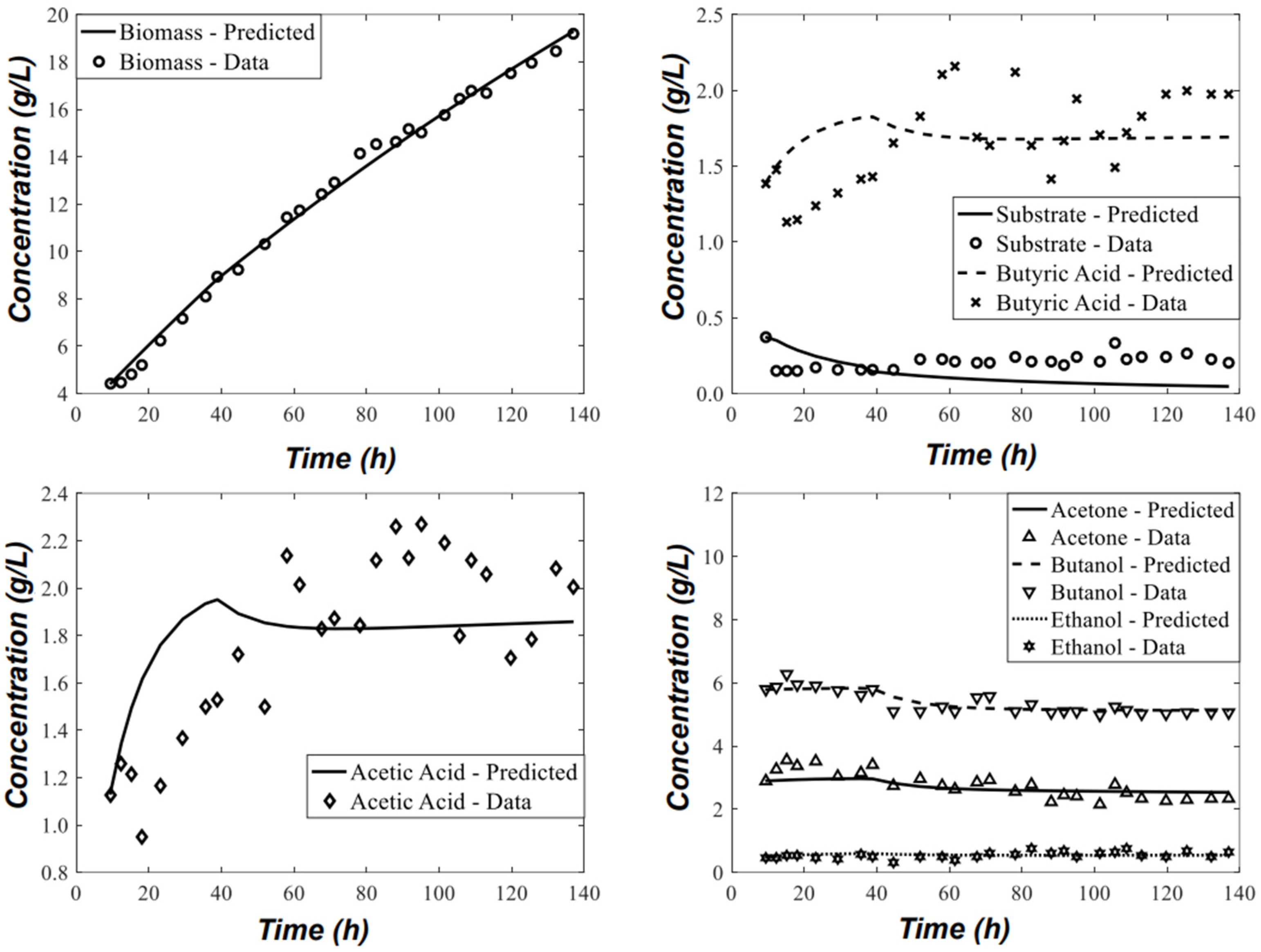
3.1. Parameter Estimation and Statistical Analysis

The ABE fermentation Base-Model—Equations (16)–(22)—was adjusted relative to experimental data via a minimization of the objective function in Equation (28), resulting in 17 parameter values shown in

Table 3. Estimated parameters for the Base-Model with 17 parameters.

Parameter Number	Parameter	Estimated Value	Unit	Confidence Interval (95% Probability)
1	${\mu }_{max}$	0.3488	h−1	$0.2833\le {\mu }_{max}\le 0.4143$
2	$k_1$	0.0588	gsubst/gcel.h	$-8.7363\le k_1\le 8.8540$
3	$k_2$	0.0972	gsubst/gcel.h	$-8.0278\le k_2\le 8.2222$
4	$Y_{X/S}$	0.0564	gcel/gsubst	$0.0214\le Y_{X/S}\le 0.0914$
5	$m$	0.0575	gsubst/gcel.h	$0.0405\le m\le 0.0745$
6	$Y_{BA/S}$	0.0573	gBA/gsubst	$0.0028\le Y_{BA/S}\le 0.1118$
7	$k_6$	0.0298	gBA/gcel.h	$-0.7728\le k_6\le 0.8323$
8	$Y_{B/S}$	0.1613	gB/gsubst	$-0.0403\le Y_{B/S}\le 0.3629$
9	$Y_{AA/S}$	0.0650	gAA/gsubst	$0.0049\le Y_{AA/S}\le 0.1252$
10	$k_9$	0.0487	gAA/gcel.h	$-0.9311\le k_9\le 0.1252$
11	$Y_{A/S}$	0.0728	gA/gsubst	$-0.0399\le Y_{A/S}\le 0.1855$
12	$Y_{E/S}$	0.0177	gE/gsubst	$0.0093\le Y_{E/S}\le 0.0262$
13	$k_{14}$	0.0967	gB/gcel.h	$-2.5875\le k_{14}\le 2.7808$
14	$k_{15}$	0.1143	gA/gcel.h	$-2.0068\le k_{15}\le 2.2355$
15	$K_S$	3.2054	g/L	$3.0614\le K_S\le 3.3493$
16	$K_{AA}$	0.3975	g/L	$-28.9374\le K_{AA}\le 29.7323$
17	$K_{BA}$	1.0405	g/L	$-8.8492\le K_{BA}\le 10.9303$

. The experimental data of observed responses of ABE fermentation come from [3]. Figure 1 shows the model regression and predicted response adherence to experimental data. Base-Model adheres satisfactorily to biomass, acetone, butanol, and ethanol curves, while acetic and butyric acid predictions could not fully represent the data throughout the fermentation time because the Base-Model predictions of acetic and butyric acids remained constant after t = 60 h, while experimental data oscillated. An important fact about ABE fermentation is that acetic and butyric acids are intermediate compounds in the production of butanol and acetone. That is, acids are produced firstly and then converted into the final products butanol and acetone. However, butanol and acetone are also produced directly from the substrate, while ethanol is only produced from the substrate. This implies that ABE fermentation has two distinct phases regarding acetic and butyric acids behaviors [3]. In the first phase, acids are produced and accumulate in the broth until certain concentrations are reached (known as the acid break), after which the conversion of acids into the final products butanol and acetone dominates until a low acid concentration is attained, which again deflagrates acid production and the cycle reinitiates. This mechanism is a possible reason for the concentration oscillation of acids around the almost constant model values. Unfortunately, it is hard for semi-empirical non-structured microbial models to capture such complex dynamics specific for intermediate acetic and butyric acids, despite the correct prediction of their average concentrations. This oscillatory behavior of acid concentrations around the model values was also observed by Mulchandani and Volesky (1986) [3] and their model also exhibited a similar shortcoming. However, the important fact with respect to the steady-state production of butanol, acetone, and ethanol via anaerobic cell-retention ABE fermentation from glucose is that the main responses are correctly predicted, such as biomass growth, substrate consumption, and butanol, acetone, and ethanol productions. That is, the model is still useful for the process analysis of ABE fermentation since solvent and biomass outputs are essentially correct, and acids are not exported; i.e., after product separation, recovered acids are returned to the fermenter because it is important to allow the microorganism to finalize its conversion into valuable solvents.

The confidence intervals of correct parameters at 95% probability and standard deviations of estimated parameters of the Base-Model with 17 parameters are shown in Figure 2 and Table 3. It is seen that there are some parameters with near zero values that have large confidence intervals (e.g., parameters No. 2, 3, 13, 14, 16, and 17). The underlying reason is related with the fact that the majority of these parameters are probably nonsignificant to the model, as confirmed in

Table 4. Fisher F test results for the 17 parameters of the Base-Model.

Parameter Number	Parameter	Test Value	Fisher Test Abscissa φ1−α	Result
1	${\mu }_{max}$	110.3981	3.8961	Significant
2	$k_1$	1.743 × 10−4	3.8961	Nonsignificant
3	$k_2$	5.576 × 10−4	3.8961	Nonsignificant
4	$Y_{X/S}$	10.1117	3.8961	Significant
5	$m$	44.4632	3.8961	Significant
6	$Y_{BA/S}$	4.3046	3.8961	Significant
7	$k_6$	0.0054	3.8961	Nonsignificant
8	$Y_{B/S}$	2.4946	3.8961	Probably Nonsignificant
9	$Y_{AA/S}$	4.5595	3.8961	Significant
10	$k_9$	0.0096	3.8961	Nonsignificant
11	$Y_{A/S}$	1.6276	3.8961	Probably Nonsignificant
12	$Y_{E/S}$	17.2535	3.8961	Significant
13	$k_{14}$	0.0051	3.8961	Nonsignificant
14	$k_{15}$	0.0113	3.8961	Nonsignificant
15	$K_S$	1931.0	3.8961	Significant
16	$K_{AA}$	7.153 × 10−4	3.8961	Nonsignificant
17	$K_{BA}$	0.0431	3.8961	Nonsignificant

. Regarding the remaining parameters, their narrow confidence intervals unveil that they are important to the model and were satisfactorily estimated with low standard deviations.

Table 4 shows the Fisher F-Test with 95% probability to assess the significance of the 17 parameters of the Base-Model. Eight parameters were spotted as definitely nonsignificant ($k_1, k_2$, $k_6, k_9$, $k_{14}, k_{15}, K_{AA}, K_{BA}$), while two are probably nonsignificant ($Y_{B/S}, Y_{A/S}$). The eight nonsignificant parameters are related to the energy requirement to produce or consume intermediate acids in the fermentation. As commented in Section 2, these acids were supposed to have adsorption on the cell wall. Hence, these nonsignificant parameters suggest that this adsorption phenomenon is not significant in a macroscopic scale, although it can be further assessed by more structured models to find internal and metabolic bottlenecks of their production and consumption. The two parameters identified as probably nonsignificant, $Y_{B/S}$ and $Y_{A/S}$, constitute a somewhat surprising outcome regarding the model structure because these parameters represent butanol and acetone production yields from the substrate and are strongly related to biochemical performances. Moreover, it can be seen in Table 4 that their significance scores are smaller than the Fisher abscissa but have the same order of magnitude, while all definitely non-significant parameters reached scores of much inferior orders of magnitude. Therefore, the status of Y_B/S and Y_A/S is a different one, and it cannot be said that they are simply nonsignificant. These parameters are important in the model because they are related to product generation directly from the substrate (i.e., not coming from the reduction of butyric and acetic acids), a phenomenon that is known to exist in ABE fermentation [3]. Thus, it is reasonable to keep these two parameters in the Reduced-Model after removing the eight definitely nonsignificant parameters.

The eight definitely nonsignificant parameters were removed from the Base-Model (i.e., were considered zero) and the remaining nine parameters were re-estimated again and statistically analyzed to re-evaluate their significance and confidence intervals. This new model with only nine adjustable parameters is the Reduced-Model. The new rate equations of the Reduced-Model after deleting the eight parameters are represented by Equations (56)–(62), with the same bioreactor dynamics in Equations (16)–(22).

$$r_x=\{\begin{array}{l}\frac{{\mu }_{max}S}{K_S+S}\mathit{exp}\left[-0.01\left(B+BA\right)\right]X, (B+BA)<8.0\mathrm{g}/\mathrm{L}\\ \frac{{\mu }_{max}S}{K_S+S}\left[2.16-0.153\left(B+BA\right)\right]X, 8.0\le \left(B+BA\right)\le 13.9\mathrm{g}/\mathrm{L}\end{array}$$

(56)

$$-r_S=\left(\frac{1}{Y_{X/S}}\mu +m\right)X$$

(57)

$$r_{AA}=\left(\frac{Y_{AA/S}}{Y_{X/S}}{\mu }_{max}\frac{S}{K_S+S}f\left(I\right)+Y_{AA/S}.m\right)X$$

(58)

$$r_{BA}=\left(\frac{Y_{BA/S}}{Y_{X/S}}{\mu }_{max}\frac{S}{K_S+S}f\left(I\right)+Y_{BA/S}.m\right)X$$

(59)

$$r_A=\left(\frac{Y_{A/S}}{Y_{X/S}}{\mu }_{max}\frac{S}{K_S+S}f\left(I\right)+Y_{A/S}.m\right)X$$

(60)

$$r_B=\left(\frac{Y_{B/S}}{Y_{X/S}}{\mu }_{max}\frac{S}{K_S+S}f\left(I\right)+Y_{B/S}.m\right)X$$

(61)

$$r_E=\left(\frac{Y_{E/S}}{Y_{X/S}}{\mu }_{max}\frac{S}{K_S+S}f\left(I\right)+Y_{E/S}.m\right)X$$

(62)

Table 5. Parameter estimation and 95% probability confidence intervals of correct parameters for the Reduced-Model with 9 parameters.

Parameter Number	Parameter	Estimated Value	Unit	Confidence Interval (95% Probability)
1	${\mu }_{max}$	0.3244	h−1	$0.2739\le {\mu }_{max}\le 0.3749$
2	$Y_{X/S}$	0.0538	gcel/gsubst	$0.0506\le Y_{X/S}\le 0.0569$
3	$m$	0.0521	gsubst/gcel.h	$0.0389\le m\le 0.0652$
4	$Y_{BA/S}$	0.0541	gBA/gsubst	$0.0481\le Y_{BA/S}\le 0.0601$
5	$Y_{B/S}$	0.1688	gB/gsubst	$0.1486\le Y_{B/S}\le 0.1890$
6	$Y_{AA/S}$	0.0582	gAA/gsubst	$0.0502\le Y_{AA/S}\le 0.0661$
7	$Y_{A/S}$	0.0854	gA/gsubst	$0.0734\le Y_{A/S}\le 0.0973$
8	$Y_{E/S}$	0.0173	gE/gsubst	$0.0161\le Y_{E/S}\le 0.0185$
9	$K_S$	2.8923	g/L	$2.8066\le K_S\le 2.9781$

shows the new estimated parameters and their confidence intervals for the Reduced-Model. Figure 3 depicts the 95% probability confidence intervals of correct parameters—in terms of percentages relative to the absolute estimated value—for the Reduced-Model with 9 parameters. All confidence intervals are narrow and well-behaved, indicating a well-posed parameter estimation of significant parameters. As can be seen in

Table 6. Fisher F test of significance for the 9 parameters of the Reduced-Model.

Parameter Number	Parameter	Test Value	Fisher Test Abscissa	Result
1	${\mu }_{max}$	160.776	3.8936	Significant
2	$Y_{X/S}$	1119.0	3.8936	Significant
3	$m$	60.746	3.8936	Significant
4	$Y_{BA/S}$	313.904	3.8936	Significant
5	$Y_{B/S}$	271.948	3.8936	Significant
6	$Y_{AA/S}$	207.651	3.8936	Significant
7	$Y_{A/S}$	198.535	3.8936	Significant
8	$Y_{E/S}$	805.819	3.8936	Significant
9	$K_S$	4430.0	3.8936	Significant

, all nine parameters of the Reduced-Model have passed the Fisher F-Test of significance with flying colors, including the two parameters, $Y_{B/S}, Y_{A/S}$, that were deemed as probably nonsignificant in the old Base-Model. Parameters $Y_{B/S}, Y_{A/S}$ regained their status in the Reduced-Model because the smaller set of parameters forced a re-distribution of importance among them, reinforcing the role of $Y_{B/S}, Y_{A/S}$ for a successful predictive performance. This is a common outcome in parameter estimation coupled to significance analysis. However, this is also a symptom that the important status of $Y_{B/S}, Y_{A/S}$ in the phenomenology of ABE fermentation was limpidly recognized in the Reduced-Model after the removal of several redundant or non-significant parameters and their associated algebraic terms. It is probable that the excessive set of 17 parameters in the Base-Model may have cloaked the critical importance of $Y_{B/S}, Y_{A/S}$ for the mechanism of butanol and acetone production, while the roles of $Y_{B/S}, Y_{A/S}$ are more evident in this mechanism in the Reduced-Model. Additionally, to represent a process with a Reduced-Model with less parameters is a positive outcome since the Reduced-Model is installable in professional simulators requiring less machine effort and that are quicker. In addition, less experimentation is required to adjust the Reduced-Model, saving bench costs and time.

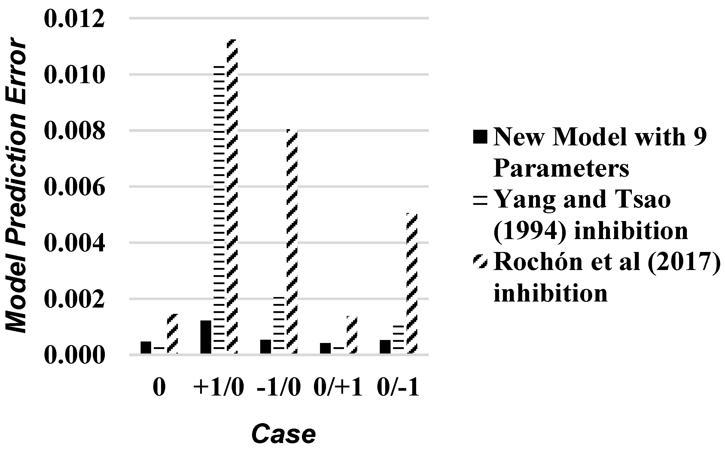
3.2. Input Variables Sensitivity Analysis

Reduced-Model, Yang–Tsao-Model, and Rochón-Model were compared in terms of the adherence of their predicted responses relative to the responses generated by the MV-Model—via the error measured by Equation (55)—under disturbances directed to the input variables specified in Table 2. In all five cases in Table 2, the simulated fermentation time was 120 h.

Figure 4 shows the average deviation via Equation (55) of each compared model—Reduced-Model, Yang–Tsao-Model, and Rochón-Model—relative to the MV-Model. Over (undisturbed) Case 0, the new Reduced-Model (9 parameters), the Yang–Tsao-Model (17 parameters), and the Rochón-Model (17 parameters) attained low errors, indicating that at these Case 0 conditions the three models behave similarly to the MV-Model.

On the other hand, on the four input disturbed cases (Table 2), only the Reduced-Model could attain a better adherence to the MV-Model, while the Yang–Tsao-Model and the Rochón-Model exhibited some lack of adherence, particularly the latter. Since the Reduced-Model has lesser parameters than the original MV-Model and also than the Yang–Tsao-Model and the Rochón-Model (these with different inhibition functions), it is evident that the Reduced-Model is the best model to use under undisturbed inputs or under disturbed inputs. In addition, the Reduced-Model will always require a lower number of experiments for calibration via parameter estimation, attaining inferior standard deviations with respect to parameters/responses and narrower correct parameter/response confidence intervals, which mean less generated uncertainty.

Among the cases in Figure 4, Case +1/0 stands out as all models attained greater errors. This can be explained by the limitations of the MV-Model [3]. The authors discuss that for feed substrate concentrations above 52 g/L, the MV-Model generated higher errors since there is no steady-state for ABE fermentation, while the predicted responses stabilize, as seen in Figure 1. Therefore, since the feed substrate concentration of Case +1/0 is close to this limit, the models may have difficulties in predicting correct concentrations, resulting in an increase in errors.

For all cases, the model with Rochón et al. (2017) [6] inhibition attained the highest errors among all models, which may entail two explanations: (i) ABE fermentation is not only inhibited by butanol, as the authors suppose, and modeling must also incorporate terms for acetic acid and butyric acid inhibitions as well; (ii) butanol is the predominant inhibition factor, as the authors suppose, but how this inhibition occurs may need a different mathematical approach. Among all models, the Reduced-Model with 9 parameters attained the best performance on the undisturbed case and on the four input-disturbed cases.

4. Conclusions

A phenomenological multi-response model was developed for ABE fermentation based on the Mulchandani and Volesky [3] ABE model. The Base-Model with 17 parameters was adjusted via the Maximum Likelihood Principle for multi-response models relative to experimental data from [3]. After statistical analysis, parameter significance tests, nonsignificant parameter deletion, and re-estimation, a tight and more compact Reduced-Model with 9 parameters was developed. This new Reduced-Model is improved compared to the Base-Model with 17 parameters because it is smaller, runs with less numerical effort, and, above all, has parameters/responses with lower standard deviations and narrower 95% probability confidence intervals for correct parameters/responses, which result in lower generated uncertainties. The Reduced-Model was compared with the Mulchandani and Volesky [3] original model and with the Base-Model using alternative inhibition functions reported in the literature. It was found that the Reduced-Model adhered well to the Mulchandani and Volesky [3] model, with improved efficiencies than the Base-Model with alternative inhibition functions. Thus, the Reduced-Model is the best substitute of the Mulchandani and Volesky [3] model and is appropriate for preliminary ABE fermentation process studies and evaluations.

References

1. Ndaba, B.; Chiyanzu, I.; Marx, S. n-Butanol derived from biochemical and chemical routes: A review. Biotechnol. Rep. 2015, 8, 1–9. [Google Scholar] [CrossRef] [Green Version]
2. Weizmann, C. Production of Acetone and Alcohol by Bacteriological Processes. US Patent 1315585A, 9 September 1919. [Google Scholar]
3. Mulchandani, A.; Volesky, B. Modelling of the acetone-butanol fermentation with cell retention. Can. J. Chem. Eng. 1986, 64, 625–631. [Google Scholar] [CrossRef]
4. Tao, L.; He, X.; Tan, E.C.D.; Zhang, M.; Aden, A. Comparative Techno-Economic Analysis and Reviews of n-Butanol Production from Corn Grain and Corn Stover. Biofuels Bioprod. Biorefining 2014, 8, 342–361. [Google Scholar] [CrossRef]
5. Yang, X.; Tsao, G.T. Mathematical modeling of inhibition kinetics in acetone-butanol fermentation by Clostridium acetobutylicum. Biotechnol. Prog. 1994, 10, 532–538. [Google Scholar] [CrossRef]
6. Rochón, E.; Ferrari, M.D.; Lareo, C. Integrated ABE fermentation-gas stripping process for enhanced butanol production from sugarcane-sweet sorghum juices. Biomass Bioenergy 2017, 98, 153–160. [Google Scholar] [CrossRef]
7. Jiang, Y.; Xu, C.; Dong, F.; Yang, Y.; Jiang, W.; Yang, S. Disruption of the acetoacetate decarboxylase gene in solvent-producing Clostridium acetobutylicum increases the butanol ratio. Metab. Eng. 2009, 11, 284–291. [Google Scholar] [CrossRef] [PubMed]
8. Jiménez-Bonilla, P.; Zhang, J.; Wang, Y.; Blersch, D.; de-Bashan, L.-E.; Guo, L.; Wang, Y. Enhancing the tolerance of Clostridium saccharoperbutylacetonicum to lignocellulosic-biomass-derived inhibitors for efficient biobutanol production by overexpressing efflux pumps genes from Pseudomonas putida. Bioresour. Technol. 2020, 312, 123532. [Google Scholar] [CrossRef]
9. Iyyappan, J.; Bharathiraja, B.; Varjani, S.; PraveenKumar, R.; Muthu Kumar, S. Anaerobic biobutanol production from black strap molasses using Clostridium acetobutylicum MTCC11274: Media engineering and kinetic analysis. Bioresour. Technol. 2021, 346, 126405. [Google Scholar] [CrossRef] [PubMed]
10. López-Linares, J.C.; García-Cubero, M.T.; Coca, M.; Lucas, S. Efficient biobutanol production by acetone-butanol-ethanol fermentation from spent coffee grounds with microwave assisted dilute sulfuric acid pretreatment. Bioresour. Technol. 2021, 320, 124348. [Google Scholar] [CrossRef]
11. Saadatinavaz, F.; Karimi, K.; Denayer, J.F.M. Hydrothermal pretreatment: An efficient process for improvement of biobutanol, biohydrogen, and biogas production from orange waste via a biorefinery approach. Bioresour. Technol. 2021, 341, 125834. [Google Scholar] [CrossRef]
12. Setlhaku, M.; Heitmann, S.; Górak, A.; Wichmann, R. Investigation of gas stripping and pervaporation for improved feasibility of two-stage butanol production process. Bioresour. Technol. 2013, 136, 102–108. [Google Scholar] [CrossRef]
13. Valles, A.; Álvarez-Hornos, J.; Capilla, M.; San-Valero, P.; Gabaldón, C. Fed-batch simultaneous saccharification and fermentation including in-situ recovery for enhanced butanol production from rice straw. Bioresour. Technol. 2021, 342, 126020. [Google Scholar] [CrossRef]
14. Mascal, M. Chemicals from biobutanol: Technologies and markets. Biofuels Bioprod. Biorefining 2012, 6, 483–493. [Google Scholar] [CrossRef]
15. Da Silva Trindade, W.R.; dos Santos, R.G. Review on the characteristics of butanol, its production and use as fuel in internal combustion engines. Renew. Sustain. Energy Rev. 2017, 69, 642–651. [Google Scholar] [CrossRef]
16. Bharathiraja, B.; Jayamuthunagai, J.; Sudharsanaa, T.; Bharghavi, A.; Praveenkumar, R.; Chakravarthy, M.; Yuvaraj, D. Biobutanol—An impending biofuel for future: A review on upstream and downstream processing tecniques. Renew. Sustain. Energy Rev. 2017, 68, 788–807. [Google Scholar] [CrossRef]
17. Papoutsakis, E.T. Equations and calculations for fermentations of butyric acid bacteria. Biotechnol. Bioeng. 1984, 26, 174–187. [Google Scholar] [CrossRef]
18. Shinto, H.; Tashiro, Y.; Yamashita, M.; Kobayashi, G.; Sekiguchi, T.; Hanai, T.; Kuriya, Y.; Okamoto, M.; Sonomoto, K. Kinetic modeling and sensitivity analysis of acetone–butanol–ethanol production. J. Biotechnol. 2007, 131, 45–56. [Google Scholar] [CrossRef]
19. Buehler, E.A.; Mesbah, A. Kinetic Study of Acetone-Butanol-Ethanol Fermentation in Continuous Culture. PLoS ONE 2016, 11, e0158243. [Google Scholar] [CrossRef]
20. Lian, T.; Zhang, W.; Cao, Q.; Wang, S.; Yin, F.; Chen, Y.; Zhou, T.; Dong, H. Optimization of lactate production from co-fermentation of swine manure with apple waste and dynamics of microbial communities. Bioresour. Technol. 2021, 336, 125307. [Google Scholar] [CrossRef]
21. Martinez-Burgos, W.J.; Sydney, E.B.; de Paula, D.R.; Medeiros, A.B.P.; de Carvalho, J.C.; Molina, D.; Soccol, C.R. Hydrogen production by dark fermentation using a new low-cost culture medium composed of corn steep liquor and cassava processing water: Process optimization and scale-up. Bioresour. Technol. 2021, 320, 124370. [Google Scholar] [CrossRef]
22. Mota, T.R.; Oliveira, D.M.; Simister, R.; Whitehead, C.; Lanot, A.; dos Santos, W.D.; Rezende, C.A.; McQueen-Mason, S.J.; Gomez, L.D. Design of experiments driven optimization of alkaline pretreatment and saccharification for sugarcane bagasse. Bioresour. Technol. 2021, 321, 124499. [Google Scholar] [CrossRef] [PubMed]
23. Velázquez-Sánchez, H.I.; Aguilar-López, R. Multi-Objective Optimization of an ABE Fermentation System for Butanol Production as Biofuel. Int. J. Chem. React. Eng. 2019, 17, 20180214. [Google Scholar] [CrossRef]
24. Eom, M.-H.; Kim, B.; Jang, H.; Lee, S.-H.; Kim, W.; Shin, Y.-A.; Lee, J.H. Dynamic Modeling of a Fermentation Process with Ex situ Butanol Recovery (ESBR) for Continuous Biobutanol Production. Energy Fuels 2015, 29, 7254–7265. [Google Scholar] [CrossRef]
25. Gattermayr, F.; Herwig, C.; Leitner, V. Effect of changes in continuous carboxylate feeding on the specific production rate of butanol using Clostridium saccharoperbutylacetonicum. Bioresour. Technol. 2021, 332, 125057. [Google Scholar] [CrossRef] [PubMed]
26. Petre, E.; Selişteanu, D.; Roman, M. Advanced nonlinear control strategies for a fermentation bioreactor used for ethanol production. Bioresour. Technol. 2021, 328, 124836. [Google Scholar] [CrossRef] [PubMed]
27. Pradhan, N.; d’Ippolito, G.; Dipasquale, L.; Esposito, G.; Panico, A.; Lens, P.N.L.; Fontana, A. Kinetic modeling of hydrogen and L-lactic acid production by Thermotoga neapolitana via capnophilic lactic fermentation of starch. Bioresour. Technol. 2021, 332, 125127. [Google Scholar] [CrossRef] [PubMed]
28. Monod, J. The Growth of Bacterial Cultures. Annu. Rev. Microbiol. 1949, 3, 371–394. [Google Scholar] [CrossRef] [Green Version]
29. Pirt, S.J. Principles of Microbe and Cell Cultivation; John Wiley & Sons: New York, NY, USA, 1975. [Google Scholar]
30. De Medeiros, J.L.; Barbosa, L.C.; Araújo, O.Q.F. Equilibrium Approach for CO2 and H2S Absorption with Aqueous Solutions of Alkanolamines: Theory and Parameter Estimation. Ind. Eng. Chem. Res. 2013, 52, 9203–9226. [Google Scholar] [CrossRef]
Figure 1. ABE fermentation Base-Model with 17 parameters: predicted concentration versus time against experimental values.
Processes 10 01978 g001
Figure 2. Correct parameters confidence interval with 95% probability for the Base-Model with 17 parameters.
Processes 10 01978 g002
Figure 3. Parameter confidence intervals for the Reduced-Model with 9 parameters (95% probability).
Processes 10 01978 g003
Figure 4. Sensitivity to input variables: adherence of Reduced-Model (9 parameters), Yang–Tsao-Model (17 parameters), and Rochón-Model (17 parameters) [6] over fermentation responses generated with the MV-Model for 120 h of ABE fermentation.
Processes 10 01978 g004