A T-S Fuzzy Quaternion-Value Neural Network-Based Data-Driven Generalized Predictive Control Scheme for Mecanum Mobile Robot

Abstract

Four-mecanum-wheeled omnidirectional mobile robots (FMOMR) are widely used in many practical scenarios because of their high mobility and flexibility. However, the performance of trajectory tracking would be degenerated largely due to various reasons. To deal with this issue, this paper proposes a data-driven algorithm by using the T-S fuzzy quaternion-value neural network (TSFQVNN). TSFQVNN is tailored to obtain the controlled autoregressive integral moving average (CARIMA) model, and then the generalized predictive controller (GPC) is designed based on the CARIMA model. In this way, the spatial relationship between the three-dimensional pose coordinates can be preserved and training times can be reduced. Furthermore, the convergence of the proposed algorithm is verified by the Stone–Weierstrass theorem, and the convergence conditions of the algorithm are discussed. Finally, the proposed control scheme is applied to the three-dimensional (3D) trajectory tracking problem on the arc surface, and the simulation results prove the necessity and feasibility of the algorithm.

1. Introduction

Nowadays, mobile robots appear in many industrial applications, such as logistics [1], the chemical industry [2,3], shopping malls [4], and other fields. Compared with four-wheel car-like mobile robots, FMOMR, due to their high mobility and flexibility, have been widely used in soccer robots, nursing robots, mobile manipulators, etc. [5,6]. However, in practical applications, FMOMR would inevitably be affected by time-delays, nonlinear frictions, and unknown external disturbances, resulting in great performance degeneration in trajectory tracking. Therefore, there are great challenges to realize accurate trajectory tracking for FMOMR [7,8].

Usually, there are at least two methods to perform the modeling work, such as black box modeling and non-black box modeling. The latter requires a clear physical model or at least structure parameters. In [9,10,11], researchers created the model for FMOMR from the point of kinematics. However, the kinematics model is not accurate enough for the existence of uncertainty. Black box modeling methods can make up for the shortcomings of mechanism modeling, and they are suitable for nonlinear system modeling, such as neural network [12,13], even though some important information can be wasted or ignored. For example, there is plenty of empirical knowledge, and rule-based information cannot be utilized by neural networks for their structure characteristic. In addition, the tool of fuzzy logic has come in vogue for solving the problem of uncertainty and nonlinearity [14,15]. Generally, the fuzzy logic system does not obtain the ability to learn, but behaves well by combining with the neural networks, such as the fuzzy differential neural network [16], the fuzzy wavelet neural network [17], and the fuzzy recurrent wavelet neural network [18]. However, the huge computation and memory demands prevent the aforementioned fuzzy neural networks from being implemented in practical systems.

In addition, in many practical applications, the ability to move along the spherical or arc surface is required, which requires taking the dynamics of FMOMR in 3D space into account. Under these circumstances, the aforementioned learning-based methods are usually simplified to multiple multi-input–single-output (MISO) systems when they are used to approximate a multi-input–multi-output (MIMO) system, which would miss the spatially structured relations among those 3D pose coordinates [19]. Recently, the quaternion neural network has been regarded as an effective method to identify 3D or four-dimensional (4D) systems [20,21]. The core idea of the quaternion neural network is to use quaternion to represent 3D or 4D input information, so as to capture the inherent structured information through Hamilton product [19]. In the meantime, a quaternion weight linking two quaternion units only has four degrees of freedom, whereas the corresponding weight parameter of standard BP neural network is $4\times 4=16$, i.e., a fourfold memory saving is achieved by using a quaternion neural network [22]. Because of these benefits, the quaternion neural network plays an important role in the field of speech recognition [23], color image compression [20], wind forecasting, etc. [24]. However, it still has the common shortcoming of the neural network, which does not have the ability to deal with uncertain information and cannot make effective use of empirical knowledge. Therefore, we consider a tailored fuzzy quaternion neural network to represent the dynamics of FMOMR with structured spatial information preserved. On the other hand, we can obtain a set of T-S fuzzy models through TSFQVNN. Then, because the consequent of the T-S fuzzy model is very similar to the CARIMA model, we can convert them into the CARIMA model. Finally, for the CARIMA model, a 3D trajectory tracking controller is designed by using multivariable generalized predictive control.

Compared to the existing works, the proposed approach has several advantages. (1) Those existing trajectory tracking control schemes for FMOMR in [7,8,25] could only realize trajectory tracking in a two-dimensional plane. This strategy realizes the trajectory tracking of FMOMR on the arc surface. (2) The proposed system identification method not only has the advantages of the fuzzy logic system and neural network, but also gives full play to the benefits of quaternion representation. In this way, the algorithm can identify 3D or 4D systems with better performance, and the number of weight updates is less than that of [12,13,14,15,16,17,18]. (3) The universal approximation of TSFQVNN is proven by the Stone–Weierstrass theorem, and its stability is analyzed by the Lyapunov theory. (4) Different from the existing fuzzy generalized predictive controller [26,27], the proposed CARIMA-based controller preserves the correlation between multi-dimensional pose coordinates. Simulation results show that the designed controller can obtain higher 3D trajectory tracking accuracy.

The rest of the paper is organized as follows. Section 2 presents a formulation of the problem. Section 3 introduces TSFQVNN. Section 4 presents the TSFQVNN-GPC. In Section 5, simulations for FMOMR 3D trajectory tracking based on TSFQVNN-GPC, are provided to show the effectiveness of the proposed method. Finally, Section 6 draws a conclusion.

2. Problem Description

In this paper, we consider the situation that the FMOMR could move on a circular arc or a spherical surface, which makes the FMOMR kinematic model a 4-input-3-output system. The input and output data come from a four rotate speed input for mecanum wheels and position output of the robot body along the x, y, and z axes among the world coordinate system. Figure 1 describes a scene in which FMOMR move on the internal surface of a cylindrical cavity. The robot mainly consists of a mobile robot body, mecanum wheels, and continuum manipulator. There are various functional devices equipped in the mobile robot body, and the four mecanum wheels can move in any direction on the surface. The continuum manipulator installed on the front of the robot body can achieve inspection operation in a spatially complex environment. At the same time, many uncertainties in FMOMR lead to a complex and imprecise modeling process. This makes it impossible to guarantee that an effective motion controller can be used for FMOMR with different structural designs. Therefore, the ”data-based“ method can be used to control the motion of the mobile robot.

First, to compensate for the lack of self-learning ability of the T-S fuzzy logic system, many researchers use the fuzzy neural network for system identification. Figure 2 describes the structure of the T-S fuzzy neural network (TSFNN). For the FMOMR system, the implementation of TSFNN requires the 4-input-3-output system to be divided into three 4-input-1-output systems. Finally, three T-S fuzzy models with 4-input-1-output can be obtained. The characteristics of T-S fuzzy model afterparts are helpful to build the CARIMA model, and then design the GPC controller based on the CARIMA model to realize FMOMR 3D trajectory tracking control.

Three T-S fuzzy models with 4-input-1-output can be obtained from TSFNN above.

$$\begin{array}{c}\hfill {\mathbb{R}}_j^r:if\begin{array}{c}u\begin{array}{c}is\end{array}\begin{array}{c}{\mu }_j\end{array}\end{array},Then\begin{array}{c}{y}_j^r(k+1)={\left(p_{0j}^r\right)}^T+{\left(p_{ij}^r\right)}^T{U}^r\end{array},\\ \hfill j=1,\cdots ,N,r=1,2,3,\end{array}$$

(1)

where $U^r=[y^r\left(k\right),y^r(k-1),\dots ,y^r(k-n_a+1),u(k-1),\dots ,u(k-n_b)]$ is the input and output variable. ${\mu }_j=[A_{1j},\dots ,A_{n_{a}j},B_{1j},\dots ,B_{n_{b}j}]$ denotes the $jth$ membership function. ${\left(p_{ij}^r\right)}^T={[a_{1j}^r,\dots ,a_{n_{a}j}^r,b_{1j}^r,\dots ,b_{n_{b}j}^r]}^T$ represents the jth consequent parameter. It can be regarded as the parameter of the jth linear submodel of the rth T-S fuzzy model.

Then the CARIMA model is obtained by weighted summation of the T-S fuzzy model above, and finally, the 3D trajectory tracking controller is designed by GPC.

3. T-S Fuzzy Quaternion-Value Neural Network Identification

In this part, TSFQVNN and its learning algorithm are introduced, and it is proven that the fuzzy neural network model can approximate any nonlinear system with any accuracy. In addition, the stability analysis is achieved by the method of Lyapunov stability analysis.

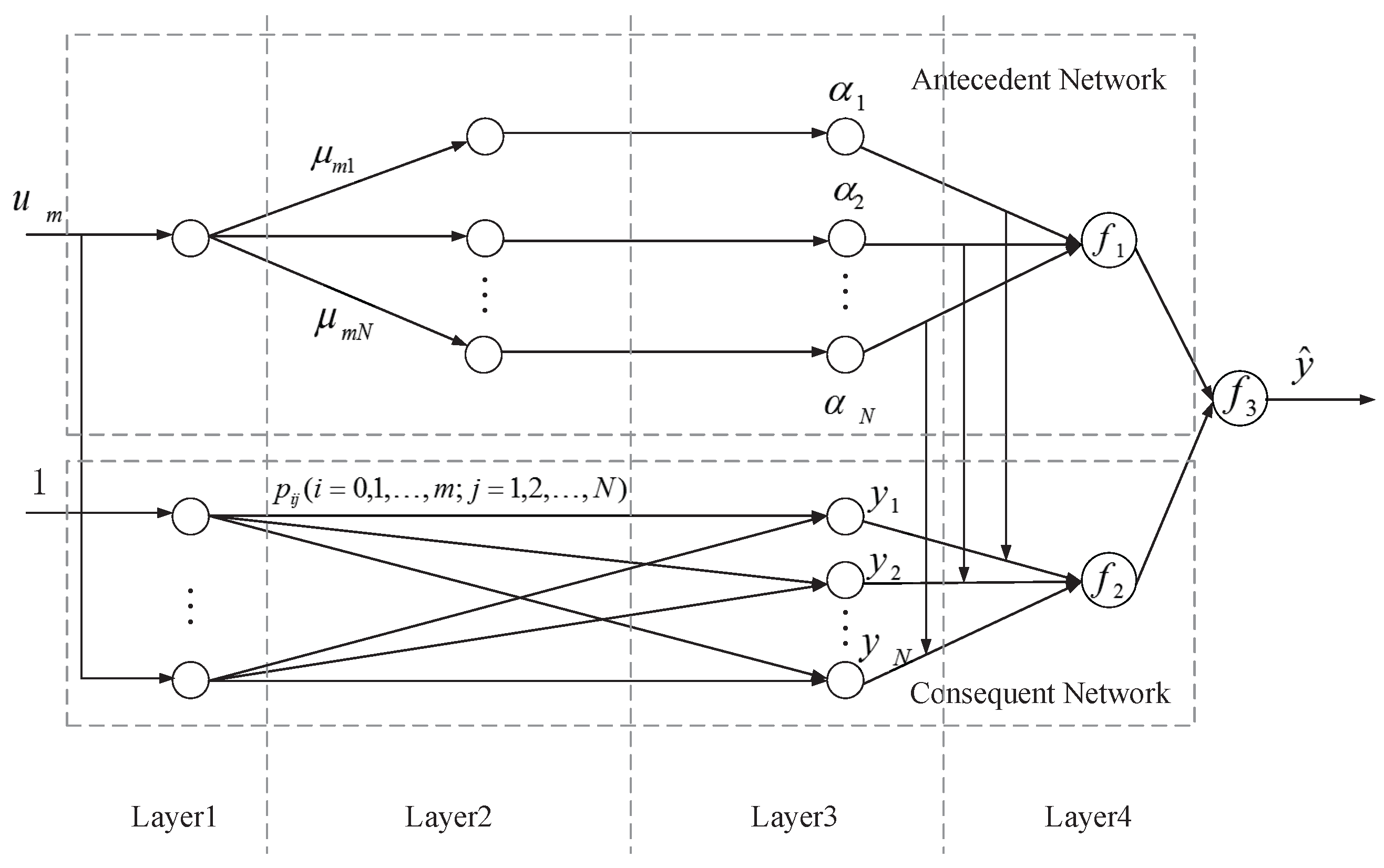
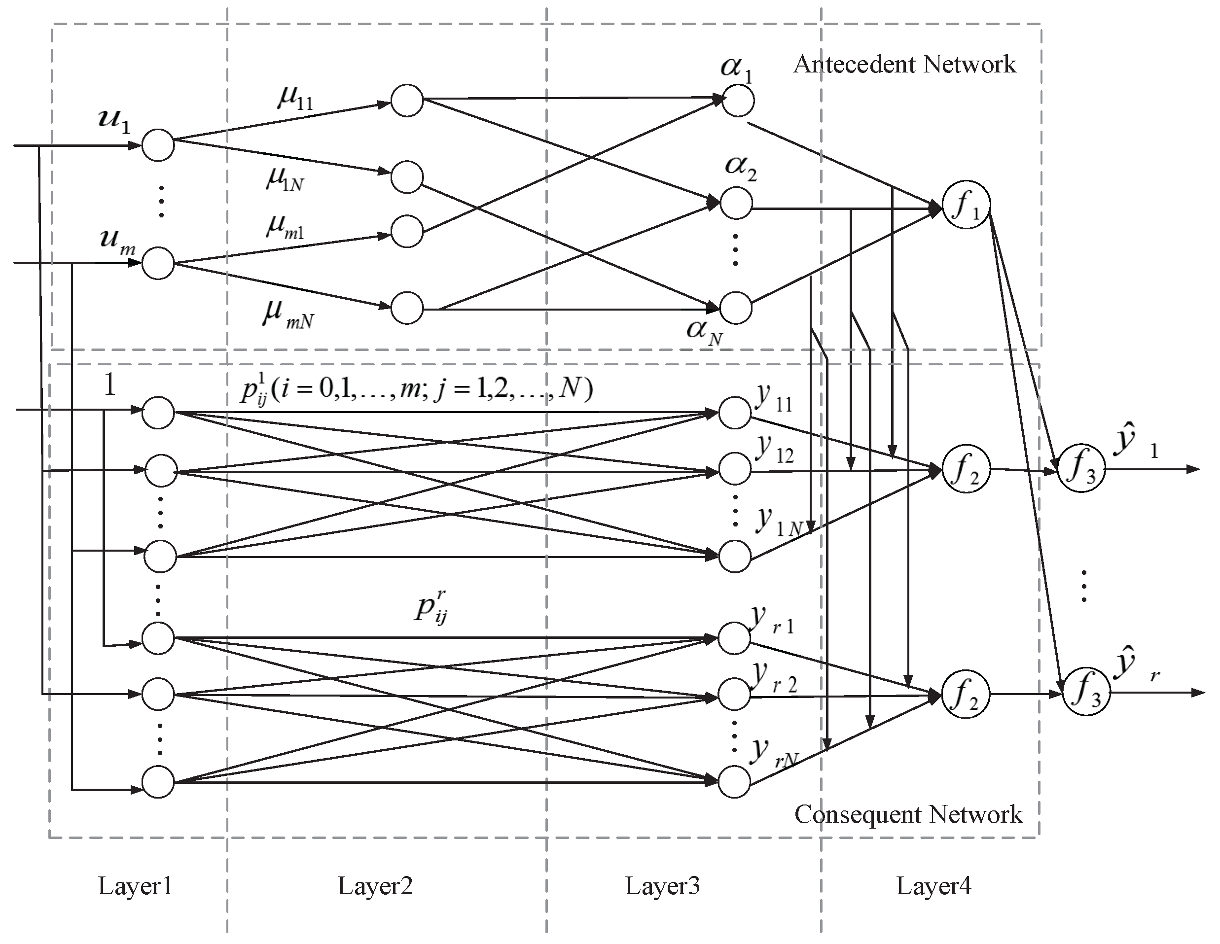
3.1. T-S Fuzzy Quaternion-Value Neural Network

First of all, a network structure is supposed to be introduced of the TSFQVNN. It has four layers, and each input and output is a quaternion neuron in Figure 3, for the sake of simplicity. Therefore, the network structure looks more concise than the TSFNN structure, and the four-layer structure of TSFQVNN is identified with the TSFNN layers structure. In the antecedent network, we do not need to divide the MIMO system into subsystems according to its dimension of input variable, but adopt the quaternion method. Furthermore, the output of the consequent network can benefit from the quaternion as well. In this way, the traditional TSFNN with quaternion-value can handle with the trajectory tracking problem in 3D space well from the degree of structured information representation and memory saving. The detailed descriptions of the four layers are as follows.

• Layer 1: The first layer is defined by N input variable $u_i$:

  $$\begin{array}{cc}\hfill u_i\left(k\right)& =u_i^{Re}+\mathbf{i}{u}_i^{Im\left(i\right)}+\mathbf{j}{u}_i^{Im\left(j\right)}+\mathbf{k}{u}_i^{Im\left(k\right)},\hfill \\ \hfill & k=1,\dots ,n,i=1,\dots ,m,\hfill \end{array}$$

  (2)

  where m and n are the dimension of input vector and order of the system, respectively.
• Layer 2: The second layer fuzzifies the data from the first layer and gets the membership function ${\mu }_{ij}(j=1,\dots ,N)$. N denotes the fuzzy partition number of $u_i$. Then, we use the Gaussian function as the split-activation function because the split-activation function can avoid a large number of singularities in the process of solving [22]. We have:

  $$\begin{array}{c}\hfill {\mu }_{ij}\left(u_i\right)=exp\left[\frac{-(\left(u_i\left(k\right)\right)-{\left(c_{ij}\right)}^2)}{\left({\sigma }_{ij}^2\right)}\right],\end{array}$$

  (3)

  where the initial values $c_{ij}^0$ and ${\sigma }_{ij}^0$ of $c_{ij}$ and ${\sigma }_{ij}$ are calculated from the fuzzy c-means (FCM) methods [28]. The formula is as follows:

  $$c_{ij}^0={\left(c_{ij}^0\right)}^{Re}+\mathbf{i}{\left(c_{ij}^0\right)}^{Im\left(i\right)}+\mathbf{j}{\left(c_{ij}^0\right)}^{Im\left(j\right)}+\mathbf{k}{\left(c_{ij}^0\right)}^{Im\left(k\right)},$$

  (4)

  $${\sigma }_{ij}^0={\left({\sigma }_{ij}^0\right)}^{Re}+\mathbf{i}{\left({\sigma }_{ij}^0\right)}^{Im\left(i\right)}+\mathbf{j}{\left({\sigma }_{ij}^0\right)}^{Im\left(j\right)}+\mathbf{k}{\left({\sigma }_{ij}^0\right)}^{Im\left(k\right)}.$$

  (5)
  The following is the real part for example, and the rest can be obtained in this way:

  $${\left(c_{ij}^0\right)}^{Re}=\frac{{\sum }_{k=1}^N{\left({\mu }_{ij}^{Re}\left(k\right)\right)}^{\varrho }{u}_i^{Re}\left(k\right)}{{\sum }_{k=1}^N{\left({\mu }_{ij}^{Re}\left(k\right)\right)}^{\varrho }},$$

  (6)

  $${\left({\sigma }_{ij}^0\right)}^{Re}=\sqrt{\frac{{\sum }_{k=1}^N{\mu }_{ij}^{Re}\left(k\right){(u_i^{Re}\left(k\right)-{\left(c_{ij}^0\right)}^{Re}\left(k\right))}^2}{{\sum }_{k=1}^N{\mu }_{ij}^{Re}\left(k\right)}},$$

  (7)

  where $\varrho ϵ(1,\infty )$ is a weighted exponent.
• Layer 3: Each node in the antecedent network represents a fuzzy rule. The fuzzy method of single point fuzzy set is adopted for the input value, namely:

  $${\alpha }_j=\prod _{i=1}^m{\mu }_{ij}^{Re}+\mathbf{i}\prod _{i=1}^m{\mu }_{ij}^{Im\left(i\right)}+\mathbf{j}\prod _{i=1}^m{\mu }_{ij}^{Im\left(j\right)}+\mathbf{k}\prod _{i=1}^m{\mu }_{ij}^{Im\left(k\right)}.$$

  (8)

  .

  $$y_j=y_j^{Re}+\mathbf{i}{y}_j^{Im\left(i\right)}+\mathbf{j}{y}_j^{Im\left(j\right)}+\mathbf{k}{y}_j^{Im\left(k\right)},$$

  (9)

  where $y_j^{Re}=p_{0j}^{Re}+p_{1j}^{Re}{u}_1^{Re}+\dots +p_{mj}^{Re}{u}_m^{Re}$.
• Layer 4: The fourth layer is the output layer and contains three functions, $f_1$, $f_2$, $f_3$. The function $f_1$ sums the fitness of the fuzzy antecedent, and then the function $f_2$ and $f_3$ can calculate the output of the system. We have

  $$f_1=\sum _{j=1}^N{\alpha }_j^{Re}+\mathbf{i}\sum _{j=1}^N{\alpha }_j^{Im\left(i\right)}+\mathbf{j}\sum _{j=1}^N{\alpha }_j^{Im\left(j\right)}+\mathbf{k}\sum _{j=1}^N{\alpha }_j^{Im\left(k\right)},$$

  (10)

  $$f_2=\sum _{j=1}^N{\alpha }_j{y}_j,$$

  (11)

  $$f_3=\frac{f_2^{Re}}{f_1^{Re}}+\mathbf{i}\frac{f_2^{Im\left(i\right)}}{f_1^{Im\left(i\right)}}+\mathbf{j}\frac{f_2^{Im\left(j\right)}}{f_1^{Im\left(j\right)}}+\mathbf{k}\frac{f_2^{Im\left(k\right)}}{f_1^{Im\left(k\right)}}.$$

  (12)
  Consequently the system forecast output is

  $$\begin{array}{cc}\hfill \widehat{y}& =\frac{{\sum }_{j=1}^N{\left({\alpha }_j\right)}^{Re}{\left(y_j\right)}^{Re}}{{\sum }_{j=1}^N{\left({\alpha }_j\right)}^{Re}}+\mathbf{i}\frac{{\sum }_{j=1}^N{\left({\alpha }_j\right)}^{Im\left(i\right)}{\left(y_j\right)}^{Im\left(i\right)}}{{\sum }_{j=1}^N{\left({\alpha }_j\right)}^{Im\left(i\right)}}\hfill \\ \hfill & +\mathbf{j}\frac{{\sum }_{j=1}^N{\left({\alpha }_j\right)}^{Im\left(j\right)}{\left(y_j\right)}^{Im\left(j\right)}}{{\sum }_{j=1}^N{\left({\alpha }_j\right)}^{Im\left(j\right)}}+\mathbf{k}\frac{{\sum }_{j=1}^N{\left({\alpha }_j\right)}^{Im\left(k\right)}{\left(y_j\right)}^{Im\left(k\right)}}{{\sum }_{j=1}^N{\left({\alpha }_j\right)}^{Im\left(k\right)}}.\hfill \end{array}$$

  (13)

The T-S fuzzy model composed of N rules can be obtained from TSFQVNN above. We have

$$\begin{array}{c}\hfill {\mathbb{R}}_j:if\begin{array}{c}u\begin{array}{c}is\end{array}\begin{array}{c}{\mu }_j\end{array}\end{array},Then\begin{array}{c}{y}_j(k+1)={\left(p_{0j}\right)}^T+{\left(p_{ij}\right)}^{T}U\end{array},\\ \hfill j=1,\cdots ,N,\end{array}$$

(14)

where $U=[y\left(k\right),y(k-1),\dots ,y(k-n_a+1),u(k-1),\dots ,u(k-n_b)]$ is the input and output variable. ${\mu }_j=[A_{1j},\dots ,A_{n_{a}j},B_{1j},\dots ,B_{n_{b}j}]$ is the jth membership function. ${\left(p_{ij}\right)}^T={[a_{1j},\dots ,a_{n_{a}j},b_{1j},\dots ,b_{n_{b}j}]}^T$ is the jth consequent parameter. It can be regarded as the parameter of the jth linear submodel.

Remark 1.

For 3D and 4D systems, TSFNN needs to update the weight three or four times, while TSFQVNN only needs to update the weight once. This makes TSFQVNN identification faster and less computational.

3.2. The Learning Algorithm

The rules for TSFQVNN learning is defined. Take the error cost function as

$$E=\frac{1}{2}\sum _{l=1}^M\mid y_l-{\widehat{y}}_l{\mid }^2,$$

(15)

where $y_i$ is reference output, ${\widehat{y}}_i$ represents forecast output, M denotes the number of output neurons, and $\left|x\right|\stackrel{def}{=}\sqrt{x_1^2+x_2^2+x_3^2+x_4^2}$ for a quaternion $x=x_1+\mathbf{i}{x}_2+\mathbf{j}{x}_3+\mathbf{k}{x}_4$.

For a sufficiently small learning constant $\epsilon >0$, and the thresholds are supposed to be updated according to the following equations:

$$\begin{array}{c}\hfill \mathrm{\Delta }{p}_{0j}\stackrel{def}{=}-\epsilon \left(\frac{\partial E}{\partial {\left(p_{0j}\right)}^{Re}}+\mathbf{i}\frac{\partial E}{\partial p_{0j}^{Im\left(i\right)}}+\mathbf{j}\frac{\partial E}{\partial p_{0j}^{Im\left(j\right)}}+\mathbf{k}\frac{\partial E}{\partial p_{0j}^{Im\left(k\right)}}\right),\end{array}$$

(16)

$$\begin{array}{cc}\hfill \mathrm{\Delta }{p}_{ij}& \stackrel{def}{=}-\epsilon \left(\frac{\partial E}{\partial p_{ij}^{Re}}+\mathbf{i}\frac{\partial E}{\partial p_{ij}^{Im\left(i\right)}}+\mathbf{j}\frac{\partial E}{\partial p_{ij}^{Im\left(j\right)}}+\mathbf{k}\frac{\partial E}{\partial p_{ij}^{Im\left(k\right)}}\right),\hfill \end{array}$$

(17)

where $\mathrm{\Delta }$ denotes the correction of a parameter, $\epsilon$ is the learning rate, and because of the complicated relationship between its size, speed and accuracy of network convergence, it is necessary to adjust the learning rate through multiple tests.

The above Equations (16) and (17) can be expressed as:

$$\mathrm{\Delta }d{p}_{ij}={\overline{f}}_2\mathrm{\Delta }d{p}_{0j},\mathrm{\Delta }d{p}_{0j}=\epsilon e_l(1-f_3)f_3,$$

(18)

where $e_l=e_l^{Re}+\mathbf{i}{e}_l^{Im\left(i\right)}+\mathbf{j}{e}_l^{Im\left(j\right)}+\mathbf{k}{e}_l^{Im\left(k\right)}=y_l-{\widehat{y}}_l$ denotes the error between ${\widehat{y}}_l$ and the target output signal $y_l$. We have

$$\mathrm{\Delta }{p}_{ij}={\overline{u}}_j\mathrm{\Delta }{p}_{0j},$$

(19)

$$\begin{array}{cc}\hfill \mathrm{\Delta }{p}_{0j}& =\left(1-f_1^{Re}\right)f_1^{Re}·Re\left[\sum _{j=1}^N(\mathrm{\Delta }d{p}_{0j}\times \mathrm{\Delta }{\overline{dp}}_{ij})\right]\hfill \\ \hfill & +\mathbf{i}\left(1-f_1^{Im\left(i\right)}\right)f_1^{Im\left(i\right)}·Im\left(i\right)\left[\sum _{j=1}^N(\mathrm{\Delta }d{p}_{0j}\times \mathrm{\Delta }{\overline{dp}}_{ij})\right]\hfill \\ \hfill & +\mathbf{j}\left(1-f_1^{Im\left(j\right)}\right)f_1^{Im\left(j\right)}·Im\left(j\right)\left[\sum _{j=1}^N(\mathrm{\Delta }d{p}_{0j}\times \mathrm{\Delta }{\overline{dp}}_{ij})\right]\hfill \\ \hfill & +\mathbf{k}\left(1-f_1^{Im\left(k\right)}\right)f_1^{Im\left(k\right)}·Im\left(k\right)\left[\sum _{j=1}^N(\mathrm{\Delta }d{p}_{0j}\times \mathrm{\Delta }{\overline{dp}}_{ij})\right],\hfill \end{array}$$

(20)

where $\overline{x}\stackrel{def}{=}{x}_1-\mathbf{i}{x}_2-\mathbf{j}{x}_3-\mathbf{k}{x}_4$, $Re\left[x\right]\stackrel{def}{=}{x}_1$, $Im\left(i\right)\left[x\right]\stackrel{def}{=}{x}_2$, $Im\left(j\right)\left[x\right]\stackrel{def}{=}{x}_3$, $Im\left(k\right)\left[x\right]\stackrel{def}{=}{x}_4$ for a quaternion $x=x_1+\mathbf{i}{x}_2+\mathbf{j}{x}_3+\mathbf{k}{x}_4$.

Therefore, by the Formulas (18)–(20), $\mathrm{\Delta }{p}_{0j}$ and $\mathrm{\Delta }{p}_{ij}$ can be simply expressed as follows, respectively. We have

$$\begin{array}{c}\hfill \mathrm{\Delta }{p}_{0j}=(1-f_1)f_1·\epsilon e_l\sum _{j=1}^N(1-f_3)f_3\times \mathrm{\Delta }{\overline{dp}}_{ij}=\epsilon e_l{f}_4,\end{array}$$

(21)

$$\begin{array}{cc}\hfill & \mathrm{\Delta }{p}_{ij}={\overline{u}}_j{e}_l{f}_4=\epsilon e_l{f}_5.\hfill \end{array}$$

(22)

In addition, the center $c_{ij}$ and width ${\sigma }_{ij}$ of membership function are further modified. The gradient descent algorithm is applied to the modification of parameters, namely:

$$\begin{array}{cc}\hfill \mathrm{\Delta }{c}_{ij}& \stackrel{def}{=}-\epsilon \left(\frac{\partial E}{\partial c_{ij}^{Re}}+\mathbf{i}\frac{\partial E}{\partial c_{ij}^{Im\left(i\right)}}+\mathbf{j}\frac{\partial E}{\partial c_{ij}^{Im\left(j\right)}}+\mathbf{k}\frac{\partial E}{\partial c_{ij}^{Im\left(k\right)}}\right),\hfill \end{array}$$

(23)

$$\begin{array}{cc}\hfill \mathrm{\Delta }{\sigma }_{ij}& \stackrel{def}{=}-\epsilon \left(\frac{\partial E}{\partial {\sigma }_{ij}^{Re}}+\mathbf{i}\frac{\partial E}{\partial {\sigma }_{ij}^{Im\left(i\right)}}+\mathbf{j}\frac{\partial E}{\partial {\sigma }_{ij}^{Im\left(j\right)}}+\mathbf{k}\frac{\partial E}{\partial {\sigma }_{ij}^{Im\left(k\right)}}\right),\hfill \end{array}$$

(24)

where j denotes the jth rule. i represents the ith input vector.

Remark 2.

Compared with the gradient descent method used in TSFNN weight updating, the Hamilton product used in TSFQVNN’s gradient descent method can capture these internal latent relations within the features of a quaternion and restore the spatial relations within 3D coordinates.

3.3. Proof of Global Approximation

Due to the application of fuzzy neural network in modeling work, it is necessary to prove its global approximation property.

Formula (13) can be treated as the set of fuzzy systems, named Y, and then Stone–Weierstrass theorem [29] is used to prove the global approximation ability of the model. First, it is proved that y satisfies the three conditions given in the Stone–Weierstrass theorem.

Lemma 1.

$(Y,d_{\infty })$is an algebra.

Proof. 

Assume $f_{11}$, $f_{22}ϵY$, which are described in detail as follows:

$$f_{11}\left(u\right)=d_1+\mathbf{i}{d}_2+\mathbf{j}{d}_3+\mathbf{k}{d}_4$$

(25)

$$f_{22}\left(u\right)=t_1+\mathbf{i}{t}_2+\mathbf{j}{t}_3+\mathbf{k}{t}_4$$

(26)

where $d_1=\frac{{\sum }_{j=1}^{N_1}{\left({\alpha }_j^1\right)}^{Re}{\left(y_j^1\right)}^{Re}}{{\sum }_{j=1}^{N_1}{\left({\alpha }_j^1\right)}^{Re}}$, $d_2=\frac{{\sum }_{j=1}^{N_1}{\left({\alpha }_j^1\right)}^{Im\left(i\right)}{\left(y_j^1\right)}^{Im\left(i\right)}}{{\sum }_{j=1}^{N_1}{\left({\alpha }_j^1\right)}^{Im\left(i\right)}}$, $d_3=\frac{{\sum }_{j=1}^{N_1}{\left({\alpha }_j^1\right)}^{Im\left(j\right)}{\left(y_j^1\right)}^{Im\left(j\right)}}{{\sum }_{j=1}^{N_1}{\left({\alpha }_j^1\right)}^{Im\left(j\right)}}$,

$d_4=\frac{{\sum }_{j=1}^{N_2}{\left({\alpha }_j^2\right)}^{Im\left(k\right)}{\left(y_j^2\right)}^{Im\left(k\right)}}{{\sum }_{j=1}^{N_2}{\left({\alpha }_j^2\right)}^{Im\left(k\right)}}$. $t_1=\frac{{\sum }_{j=1}^{N_2}{\left({\alpha }_j^2\right)}^{Re}{\left(y_j^2\right)}^{Re}}{{\sum }_{j=1}^{N_2}{\left({\alpha }_j^2\right)}^{Re}}$, $t_2=\frac{{\sum }_{j=1}^{N_2}{\left({\alpha }_j^2\right)}^{Im\left(i\right)}{\left(y_j^2\right)}^{Im\left(i\right)}}{{\sum }_{j=1}^{N_2}{\left({\alpha }_j^2\right)}^{Im\left(i\right)}}$,

$t_3=\frac{{\sum }_{j=1}^{N_2}{\left({\alpha }_j^2\right)}^{Im\left(j\right)}{\left(y_j^2\right)}^{Im\left(j\right)}}{{\sum }_{j=1}^{N_2}{\left({\alpha }_j^2\right)}^{Im\left(j\right)}}$, $t_4=\frac{{\sum }_{j=1}^{N_2}{\left({\alpha }_j^2\right)}^{Im\left(k\right)}{\left(y_j^2\right)}^{Im\left(k\right)}}{{\sum }_{j=1}^{N_2}{\left({\alpha }_j^2\right)}^{Im\left(k\right)}}$.

Thereupon:

$$\begin{array}{cc}\hfill f_{11}\left(u\right)\times f_{22}\left(u\right)& =(d_1{t}_1-d_2{t}_2-d_3{t}_3-d_4{t}_4)+\mathbf{i}(d_2{t}_1+d_1{t}_2+d_3{t}_4-d_4{t}_3)\hfill \\ \hfill & +\mathbf{j}(d_3{t}_1+d_1{t}_3+d_4{t}_2-d_2{t}_4)+\mathbf{k}(d_4{t}_1+d_1{t}_4+d_2{t}_3-d_3{t}_2).\hfill \end{array}$$

(27)

Because ${\mu }_{ij}^1\left(u_i\right)$ and ${\mu }_{ij}^2\left(u_i\right)$ are of Gaussian type, their product ${\alpha }_j^1$ and ${\alpha }_j^2$ are also of Gaussian type. Therefore, the form of Equation (27) is completely equivalent to that of Equation (13). It can be seen that

$$f_{11}\left(u\right)\times f_{22}\left(u\right)ϵY.$$

(28)

Furthermore, we can also get $q{f}_{11}\left(u\right)ϵY$ and $f_{11}\left(u\right)+f_{22}\left(u\right)ϵY$. So far, Lemma 1 is proven.

Lemma 2.

$(Y,d_{\infty })$can separate points on U.

Proof. 

Construct a f to prove the above conditions, that is, given the number of fuzzy sets defined on U and R, the Gauss membership function parameters, the rules number, and the rules expression, so that the f (in the form of the Formula (13)) obtained has the following characteristics:

(1) For any given $u^0$, $u{1}^0ϵU$, when $u^0\ne u{1}^0$, there is $f\left(u^0\right)\ne f\left(u{1}^0\right)$.

Set $u^0=(u_1^0,\dots ,u_m^0)$, $u{1}^0=(u{1}_1^0,\dots ,u{1}_m^0)$. If $u_i^0\ne u{1}_i^0$, two fuzzy sets $(A_i^1,{\mu }_{A_i}^1)$ and $(A_i^2,{\mu }_{A_i}^2)$ are defined in the ith subspace of U, and their corresponding membership functions are: ${\mu }_{A_i}^1\left(u_i\right)=exp\left(-\frac{{\left(\left(u_i\right)-\left(u_i^0\right)\right)}^2}{2}\right)$, ${\mu }_{A_i}^2\left(u_i\right)=exp\left(-\frac{{\left(\left(u_i\right)-\left(u{1}_i^0\right)\right)}^2}{2}\right)$.

If $u^0=u{1}^0$, there are $A_i^1=A_i^2$ and ${\mu }_{A_i}^1={\mu }_{A_i}^2$. Two fuzzy sets $(B_i^1,{\mu }_B^1)$ and $(B_i^2,{\mu }_B^2)$ are defined on the output domain R, and their corresponding membership functions are as follows:

$$\begin{array}{c}\hfill {\mu }_B^j\left(u_i\right)=exp\left(-\frac{{(y-y_j)}^2}{2}\right),\end{array}$$

(29)

where $j=1,2$, $y_j$.

Then we get the function f with the form shown in formula (30), and its expression is as follows:

$${\mu }_{A_i}^1\left(u^0\right)=1+\mathbf{i}+\mathbf{j}+\mathbf{k},$$

(30)

$$\begin{array}{cc}\hfill {\mu }_{A_i}^1\left(u{1}^0\right)& =exp\left(-\frac{{(u{1}^0-u_i^0)}^2}{2}\right).\hfill \end{array}$$

(31)

The same can be get ${\mu }_{A_i}^2\left(u^0\right)$ and ${\mu }_{A_i}^2\left(u{1}^0\right)$. Then:

$$f\left(u^0\right)=y_1+Q{\left(y_2\right)}^{Re}+R{\left(y_2\right)}^{Im\left(i\right)}+S{\left(y_2\right)}^{Im\left(j\right)}+T{\left(y_2\right)}^{Im\left(k\right)},$$

(32)

$$f\left(u{1}^0\right)=Q{\left(y_1\right)}^{Re}+R{\left(y_1\right)}^{Im\left(i\right)}+S{\left(y_1\right)}^{Im\left(j\right)}+T{\left(y_1\right)}^{Im\left(k\right)}+y_2,$$

(33)

Suppose $f\left(u^0\right)=f\left(u{1}^0\right)$. Then we have

$$\begin{array}{cc}\hfill f\left(u^0\right)=f\left(u{1}^0\right)& \Rightarrow (1-Q)({\left(y_1\right)}^{Re}-{\left(y_2\right)}^{Re})+(1-R)({\left(y_1\right)}^{Im\left(i\right)}-{\left(y_2\right)}^{Im\left(i\right)})\hfill \\ \hfill & +(1-S)({\left(y_1\right)}^{Im\left(j\right)}-{\left(y_2\right)}^{Im\left(j\right)})+(1-T)({\left(y_1\right)}^{Im\left(k\right)}-{\left(y_2\right)}^{Im\left(k\right)})=0.\hfill \end{array}$$

(34)

Then, we can take $y_1=2+2\mathbf{i}+2\mathbf{j}+2\mathbf{k}$, $y_2=1+\mathbf{i}+\mathbf{j}+\mathbf{k}$, and there must be

$$\begin{array}{cc}& (1-Q)({\left(y_1\right)}^{Re}-{\left(y_2\right)}^{Re})+(1-R)({\left(y_1\right)}^{Im\left(i\right)}-{\left(y_2\right)}^{Im\left(i\right)})\hfill \\ & +(1-S)({\left(y_1\right)}^{Im\left(j\right)}-{\left(y_2\right)}^{Im\left(j\right)})+(1-T)({\left(y_1\right)}^{Im\left(k\right)}-{\left(y_2\right)}^{Im\left(k\right)})\ne 0,\hfill \end{array}$$

which contradicts the hypothesis, and $f\left(u^0\right)=f\left(u{1}^0\right)$ is proven.

Lemma 2 proves the end.

Lemma 3.

All points on $(Y,d_{\infty })$ are not zero.

Proof. 

Observing formula (13) carefully, just select $y_j>0,j=1,2,\dots ,N$. Any corresponding $fϵY$ can be used as the required f.

This lemma has been proven.

Theorem 1.

The TSFQVNN shown in Figure 2 is a global approximator.

Proof. 

Y is a continuous and real function from Formula (25). It is easy to deduce the global approximation ability through the lemmas mentioned above.

3.4. Stability Analysis

The direct method of Lyapunov stability analysis is a universal and effective method to analyze the stability and convergence. There are two ways to derive it; one is the convergence of the weight vector, and the other is the convergence of the output error. The latter method is used here.

In order to obtain the stability conditions of the learning algorithm, the Lyapunov function is selected as follows:

$$V\left(k\right)=\frac{1}{2}{\overline{e}}_l\left(k\right)e_l\left(k\right)=\frac{1}{2}\overline{[y_l\left(k\right)-{\widehat{y}}_l\left(k\right)]}[y_l\left(k\right)-{\widehat{y}}_l\left(k\right)],$$

(35)

where $y_l\left(k\right)$ is the lth reference output, $\widehat{y_l}\left(k\right)$ denotes the lth forecasted output.

The difference of Lyapunov function from k step to $k+1$ step is

$$\mathrm{\Delta }V\left(k\right)=V(k+1)-V\left(k\right)=\frac{1}{2}[{\overline{e}}_l(k+1)e_l(k+1)-{\overline{e}}_l\left(k\right)e_l\left(k\right)].$$

(36)

We assume that the reference output $y\left(k\right)$ is constant; then

$$\begin{array}{cc}\hfill e_l\left(k\right)& =y_l\left(k\right)-{\widehat{y}}_l\left(k\right)=y_l\left(k\right)-\frac{{\sum }_{j=1}^N\left[{\alpha }_j{\sum }_{j=1}^N(p_{0j}\left(k\right)+p_{ij}\left(k\right)u_i)\right]}{{\sum }_{j=1}^N{\alpha }_j}.\hfill \end{array}$$

(37)

From Equation (1) minus Equation (2), we have

$$\begin{array}{cc}\hfill \mathrm{\Delta }{e}_l\left(k\right)& =e_l(k+1)-e_l\left(k\right)=-\epsilon \frac{{\sum }_{j=1}^N\left[{\alpha }_j{\sum }_{j=1}^N(e_l{f}_4+e_l{f}_5{u}_i)\right]}{{\sum }_{j=1}^N{\alpha }_j}.\hfill \end{array}$$

(38)

Consequently, we have

$$\begin{array}{cc}\hfill \mathrm{\Delta }V\left(k\right)& =\frac{1}{2}[{\overline{e}}_l(k+1)e_l(k+1)-{\overline{e}}_l\left(k\right)e_l\left(k\right)]=\frac{1}{2}[({\overline{e}}_l\left(k\right)-\mathrm{\Delta }{\overline{e}}_l\left(k\right))(e_l\left(k\right)+\mathrm{\Delta }{e}_l\left(k\right))-{\overline{e}}_l\left(k\right)e_l\left(k\right)]\hfill \\ \hfill & =-\frac{\epsilon {\overline{e}}_l\left(k\right)e_l\left(k\right){\sum }_{j=1}^N\left[{\alpha }_j{\sum }_{j=1}^N(f_4+f_5{u}_i)\right]}{{\sum }_{j=1}^N{\alpha }_j}·\left[1-\frac{\epsilon {\sum }_{j=1}^N\left[{\alpha }_j{\sum }_{j=1}^N(f_4+f_5{u}_i)\right]}{2{\sum }_{j=1}^N{\alpha }_j}\right].\hfill \end{array}$$

(39)

Because $V\left(k\right)$ is positive definite, it can be seen from Lyapunov stability theorem that to make the learning process convergent and stable, $\mathrm{\Delta }V\left(k\right)$ must be positive-definite, that is, $\mathrm{\Delta }V\left(k\right)>0$. That is to say, the learning rate $\epsilon$ must meet the following requirements:

$$0<\epsilon <\frac{2{\sum }_{j=1}^N{\alpha }_j}{{\sum }_{j=1}^N\left[{\alpha }_j{\sum }_{j=1}^N(f_4+f_5{u}_i)\right]}.$$

(40)

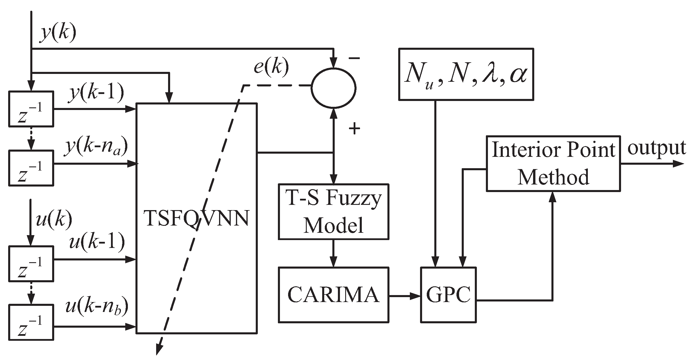
4. Fuzzy Predictive Control Algorithm

The multi-step T-S fuzzy model can be obtained from Formula (14) in section III:

$$y(k+1)=\sum _{t=1}^{n_a}{\overline{a}}_t\left(k\right)y(k-t+1)+\sum _{t=1}^{n_b}{\overline{b}}_t\left(k\right)u(k-t+1)+\overline{p}\left(k\right),$$

(41)

where, ${\overline{a}}_t\left(k\right)=\frac{{\sum }_{j=1}^N{\alpha }_j{a}_{jt}}{{\sum }_{j=1}^N{\alpha }_j}$, ${\overline{b}}_t\left(k\right)=\frac{{\sum }_{j=1}^N{\alpha }_j{b}_{jt}}{{\sum }_{j=1}^N{\alpha }_j}$, $\overline{p}\left(k\right)=\frac{{\sum }_{j=1}^N{\alpha }_j{p}_{0j}}{{\sum }_{j=1}^N{\alpha }_j}$, and each of these elements is a quaternion.

The CARIMA model can be used to obtain

$$A\left(z^{-1}\right)y\left(k\right)=B\left(z^{-1}\right)u(k-1)+\overline{p},$$

(42)

where $A\left(z^{-1}\right)$ and $B\left(z^{-1}\right)$ are as follows:

$$\left\{\begin{array}{c}A\left(z^{-1}\right)=1+a_1{z}^{-1}+\cdots +a_{n_a}{z}^{-n_a},\hfill \\ B\left(z^{-1}\right)=b_0+b_1{z}^{-1}+\cdots +b_{n_b}{z}^{-n_b}.\hfill \end{array}\right.$$

Then the control variable of $N_u$ is searched to minimize the error.

According to Section III, the CARIMA model of MIMO system can be obtained, and its objective function can be expressed as

$$J=\sum _{j=1}^{N_p}{\parallel y(k+j)-w(k+j)\parallel }^2+\sum _{j=1}^{N_u}{\parallel \mathrm{\Delta }u(k+j-1)\parallel }_{\lambda }^2,$$

(43)

where $y(k+j)$ represents the output after j step, and $w(k+j)$ denotes the desired trajectory. $N_p$ and $N_u$ are the prediction time domain and the control time domain, respectively. After $N_u$ step, u will not change; $\lambda$ is the control weighted matrix $n\times n$, namely $\lambda =diag({\lambda }_1,{\lambda }_2,\dots ,{\lambda }_n)$.

Introducing the polynomial equation of diophantine matrix: $I=E_j\left(z^{-1}\right)A\left(z^{-1}\right)\mathrm{\Delta }\left(z^{-1}\right)+z^{-j}{F}_j\left(z^{-1}\right)$, $E_j\left(z^{-1}\right)B\left(z^{-1}\right)=G_j\left(z^{-1}\right)+z^{-j}{H}_j\left(z^{-1}\right)$, where $j=1,\dots ,N_p$,

$$\left\{\begin{array}{c}{E}_j\left(z^{-1}\right)=E_0+E_1{z}^{-1}+\dots +E_{j-1}{z}^{-(j-1)},\hfill \\ F_j\left(z^{-1}\right)=F_0^j+F_1^j{z}^{-1}+\dots +F_{n_a}^j{z}^{-\left(n_a\right)},\hfill \\ G_j\left(z^{-1}\right)=G_0+G_1{z}^{-1}+\dots +G_{j-1}{z}^{-(j-1)},\hfill \\ H_j\left(z^{-1}\right)=H_0^j+H_1^j{z}^{-1}+\dots +H_{n_b-1}^j{z}^{-(n_b-1)}.\hfill \end{array}\right.$$

(44)

Multiplying both sides of Equation (44) by $E_j\left(z^{-1}\right)$, we use the diophantine equation to get

$$y(k+j)=G_j\mathrm{\Delta }u(k+j-1)+H_j\mathrm{\Delta }u(k-1)+F_{j}y\left(k\right).$$

(45)

The reference track $w(k+j)$, as shown in the following formula:

$$w(k+j)=\delta y\left(k\right)+(1-\delta )y_r,$$

(46)

where $\delta$ is the softening coefficient, from 0 to 1.

The target function can be written as

$$J={\parallel y-w\parallel }^2+{\parallel \mathrm{\Delta }u\parallel }_{\lambda }^2.$$

(47)

Next, the optimal solution is solved. First, assuming that function $h\left(\tau \right)$ satisfies:

• ${lim}_{\tau \to 0^{+}}h\left(\tau \right)=+\infty$.
• $h\left(\tau \right)>0,\forall \tau >0$.
• $h\left({\tau }_1\right)\ge h\left({\tau }_2\right),\forall {\tau }_1\le {\tau }_2$.

where ${\tau }_i\left(u\right)\ge 0$, $i=1,\dots ,m$

Taking $h\left(\tau \right)$ as the penalty term to construct the interior point penalty function

$$P_{\zeta }\left(u\right)=J\left(u\right)+{\zeta }^{-1}\sum _{i=1}^{m}h\left({\tau }_i\left(u\right)\right).$$

(48)

The optimization problems are as follows:

$$\underset{uϵR^n}{lim}{P}_{{\zeta }_k}\left(u\right)=J\left(u\right)+{\zeta }_k^{-1}\sum _{i=1}^{m}h\left({\tau }_i\left(u\right)\right),$$

(49)

where ${\zeta }_k^{-1}$ satisfies ${\zeta }_1^{-1}>\cdots >{\zeta }_k^{-1}>\cdots >0$.

It can be seen that the influence of penalty term is gradually decreasing and tends to 0.

$J\left(u\right)$, $h\left({\tau }_i\left(u\right)\right)$ and $P_{{\zeta }_k}\left(u\right)$ is supposed to convex function, and then the Newton step size of problem (49) is

$$d_k=-{\left[{\nabla }^2{P}_{{\zeta }_k}\left(u_k\right)\right]}^{-1}\nabla P_{{\zeta }_k}\left(u_k\right).$$

(50)

The penalty items is ${\zeta }^{-1}{\sum }_{i=1}^m\frac{1}{{\tau }_i\left(u\right)}$. Making $\frac{\partial P}{\partial u}=0$, we can get

$$G^{T}Gu+f{G}^T-\omega G^T+\lambda u-{\zeta }^{-1}\sum _{i=1}^m\frac{1}{{\left({\tau }_i\left(u\right)\right)}^2}=0,$$

(51)

where $f=H\mathrm{\Delta }u(k-1)+Fy$, ${\zeta }^{-1}=[1,0.1,0.01,\dots ]$

Then we get the control law for the multi-variable GPC:

$$u={(G^{T}G+I\lambda )}^{-1}(D+\zeta G^T-f{G}^T),$$

(52)

where $D=-{\zeta }^{-1}{\sum }_{i=1}^m\frac{1}{{\left({\tau }_i\left(u\right)\right)}^2}$.

Let us take the first row of ${(G^{T}G+I\lambda )}^{-1}$ and call it $P^T=[P_1,\dots ,P_{N_p}]$. Then, the generalized predictive control law can be written as follows:

$$\mathrm{\Delta }u\left(k\right)=P^T(D+\omega G^T-f{G}^T),$$

(53)

$$u(k+1)=u\left(k\right)+\mathrm{\Delta }u\left(k\right).$$

(54)

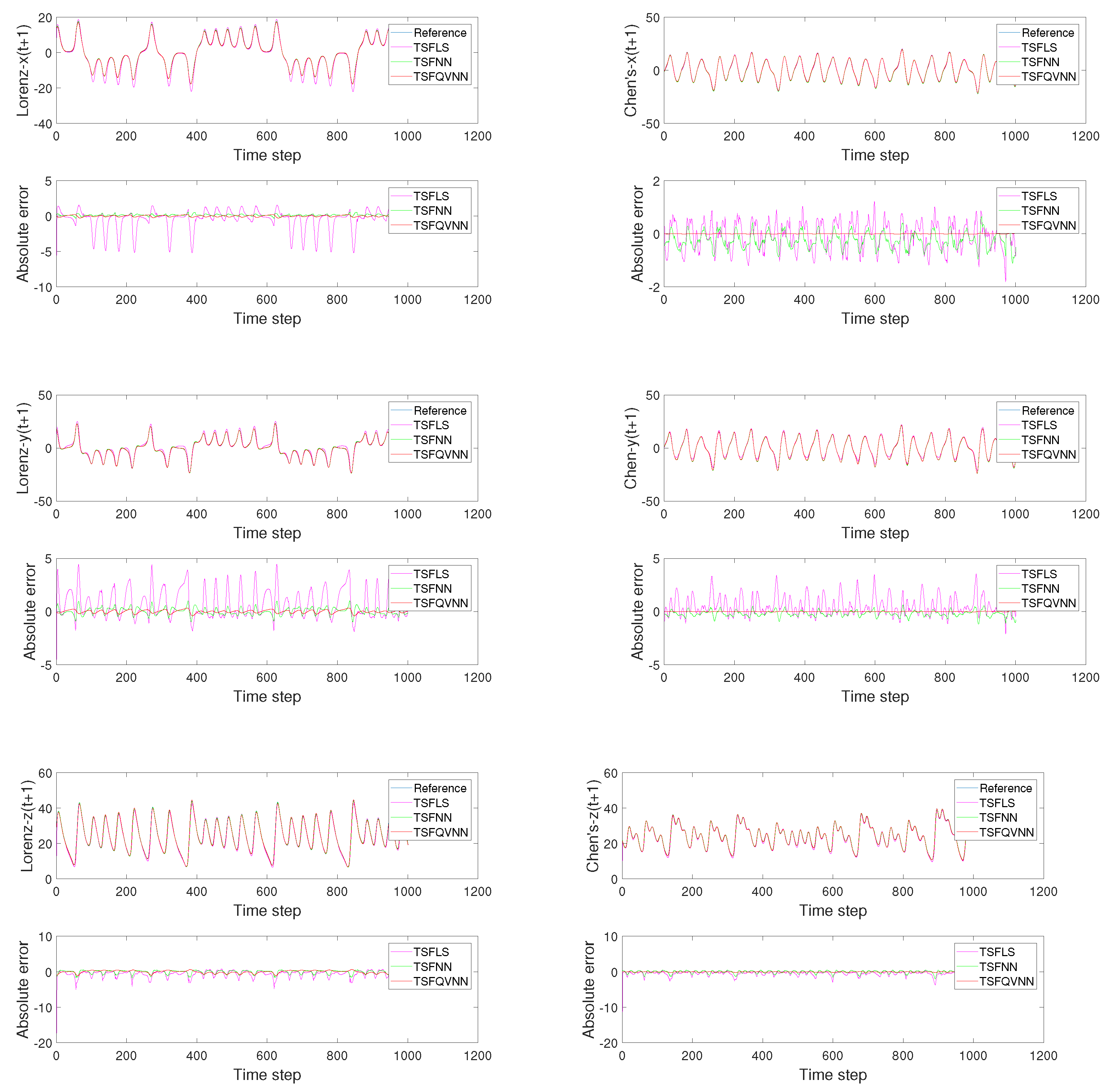
5. Simulation Results

In this section, the system identification of the FMOMR and the 3D trajectory tracking control simulation results are discussed in detail. Figure 4 shows the control flow of the algorithm proposed in paper. Firstly, the training data pairs $y\left(t\right)$ and $u\left(t\right)$ of FMOMR are sent to the TSFQVNN for training the network. Both $y\left(t\right)$ and $u\left(t\right)$ are consisted of quaternion value data. Then, the T-S fuzzy model is constructed by the TSFQVNN. Thirdly, the weighted sum of the T-S fuzzy model is used to get the CARIMA model. Finally, the GPC is designed and the objective function is optimized respectively.

5.1. System Identification

First, this paper adopts the Lorenz chaotic time series proposed by Edward Lorenz [30], and Chen’s chaotic time series proposed by Chen [31]. Chaotic time series have non-periodicity and randomness, which can effectively verify the feasibility and test the performance of TSFQVNN.

The Lorenz equation is given below [30]:

$$\begin{array}{c}\hfill \frac{dx\left(t\right)}{dt}={\varphi }_1[y\left(t\right)-x\left(t\right)],\frac{dy\left(t\right)}{dt}=x\left(t\right)[{\phi }_1-z\left(t\right)]-y\left(t\right),\frac{dz\left(t\right)}{dt}=x\left(t\right)y\left(t\right)-{\psi }_{1}z\left(t\right).\end{array}$$

(55)

Chen’s equation is given below [31]:

$$\begin{array}{c}\hfill \frac{dx\left(t\right)}{dt}={\varphi }_2[y\left(t\right)-x\left(t\right)],\frac{dy\left(t\right)}{dt}=x\left(t\right)[{\psi }_2-{\varphi }_2-z\left(t\right)]+{\psi }_{2}y\left(t\right),\frac{dz\left(t\right)}{dt}=x\left(t\right)y\left(t\right)-{\phi }_{2}z\left(t\right),\end{array}$$

(56)

where ${\varphi }_1$, ${\phi }_1$, ${\psi }_1$, ${\varphi }_2$, ${\phi }_2$, ${\psi }_2$ are the dimensionless parameters, and their typical values are used where ${\varphi }_1=10$, ${\phi }_1=28$, ${\psi }_1=8/3$, ${\varphi }_2=35$, ${\phi }_2=3$, ${\psi }_2=28$.

All the three coordinates are selected, and 3000 samples are obtained. Samples from No. 1 to No. 1840 are selected as the training data and data from No. 1841 to No. 2840 is chosen as the test set. The TSQVNN model predicts at the same time the three chaotic outputs $x(t+1)$, $y(t+1)$, and $z(t+1)$ using one quaternion’s input that contains $x\left(t\right)$, $y\left(t\right)$, and $z\left(t\right)$.

The T-S fuzzy logic system (TSFLS) model and TSFNN model are used for comparing the difference of output with TSFQVNN model. The root mean square error (RMSE), the symmetric mean absolute percentage error (SMAPE), and the normalized RMSE (NRMSE) are applied for evaluating the prediction model performance [32]. From the results of

Table 1. Comparison of performance on Lorenz series prediction.

Series	Method		RMSE	SMAPE	NRMSE
Lorenz −x(t+1)	TSFLS	ave.	0.1308	0.0143	$2.6706\times {10}^{-4}$
		std.	$2.9804\times {10}^{-4}$	$4.9069\times {10}^{-5}$	$1.2154\times {10}^{-6}$
	TSFNN	ave.	0.7136	0.0465	0.0079
		std.	0.0707	0.0046	$7.8721\times {10}^{-4}$
	TSFQVNN	ave.	0.0632	0.0037	$7.6470\times {10}^{-5}$
		std.	$7.0648\times {10}^{-4}$	$7.6684\times {10}^{-5}$	$8.3994\times {10}^{-8}$
Lorenz −y(t+1)	TSFLS	ave.	0.2796	0.0330	0.0010
		std.	0.0081	$9.8812\times {10}^{-4}$	$6.1224\times {10}^{-5}$
	TSFNN	ave.	0.9233	0.0543	0.0112
		std.	0.0915	0.0054	0.0011
	TSFQVNN	ave.	0.1008	0.0064	$1.6670\times {10}^{-4}$
		std.	0.0022	$1.9541\times {10}^{-4}$	$3.6935\times {10}^{-7}$
Lorenz −z(t+1)	TSFLS	ave.	0.4901	0.0140	0.0033
		std.	0.0081	0.0021	0.0018
	TSFNN	ave.	0.4959	0.0083	0.0031
		std.	0.0492	$8.2122\times {10}^{-4}$	$3.1080\times {10}^{-4}$
	TSFQVNN	ave.	0.1119	0.0016	$1.7078\times {10}^{-4}$
		std.	0.0022	$1.6465\times {10}^{-4}$	$1.9180\times {10}^{-5}$

and

Table 2. Comparison of performance on Chen series prediction.

Series	Method		RMSE	SMAPE	NRMSE
Chen −x(t + 1)	TSFLS	ave.	0.1396	0.0064	$2.4755\times {10}^{-4}$
		std.	0.0032	$1.7751\times {10}^{-4}$	$1.1356\times {10}^{-5}$
	TSFNN	ave.	1.0863	0.0606	0.0150
		std.	0.0029	$1.8568\times {10}^{-4}$	$7.9359\times {10}^{-6}$
	TSFQVNN	ave.	0.0037	$1.7592\times {10}^{-4}$	$1.8488\times {10}^{-7}$
		std.	0.0016	$7.6684\times {10}^{-5}$	$1.9952\times {10}^{-7}$
Chen −y(t + 1)	TSFLS	ave.	0.1690	0.0065	$3.0051\times {10}^{-4}$
		std.	0.0023	$3.9201\times {10}^{-5}$	$8.2060\times {10}^{-6}$
	TSFNN	ave.	1.4721	0.0711	0.0228
		std.	0.0046	$2.2327\times {10}^{-4}$	$1.4459\times {10}^{-4}$
	TSFQVNN	ave.	0.0081	$3.5710\times {10}^{-4}$	$7.2862\times {10}^{-7}$
		std.	0.0463	0.0014	$1.1083\times {10}^{-8}$
Chen −z(t + 1)	TSFLS	ave.	0.4379	0.0110	0.0020
		std.	0.0269	$1.9368\times {10}^{-6}$	$3.0995\times {10}^{-7}$
	TSFNN	ave.	0.4379	0.0065	0.0024
		std.	0.0046	$5.9560\times {10}^{-5}$	$7.2265\times {10}^{-5}$
	TSFQVNN	ave.	0.2644	0.0043	0.0012
		std.	0.0463	0.0028	0.0013

, it can be concluded that the proposed TSFQVNN performs better under those evaluation functions. In addition, in TSFQVNN, when the number of input/output is reduced to 1/1, only one weight update is needed. In other strategies, the number of input/output is 3/3. When it is converted to three 3/1 systems, three weight updates are needed, which requires more calculation.

Figure 5 is the prediction curve and error curve of the Lorenz series and Chen’s series generated by TSFLS, TSFNN, and TSFQVNN. The smaller error in the curve proves that the TSFQVNN can obtain 3D and 4D system information better than other methods.

Finally, it is not difficult to conclude that the TSFQVNN generates smaller averages error and standard deviation. We tend to attribute the good performance of TSFQVNN to the advantage of quaternion representation of multidimensional input and output data and the effective characteristics obtained by Hamilton product. It is specially designed for 3D and 4D system identification.

We used a virtual robot experimentation platform (CoppeliaSim) software to design an FMOMR. In addition, a narrow horizontal pipe space with three cylinders parallel to the pipe length is simulated, and an obstacle is designed at the bottom of the pipe. The purpose of the experiment is to let FMOMR bypass the obstacle and pass through the whole pipe.

5.2. Trajectory Tracking in 3D Space

First, we get a set of motion data pairs of FMOMR from the FMOMR simulation model established by CoppeliaSim software, and then use the method described in Section 3 to fit the nonlinear system. The identification results are shown in Figure 6. As you can see from Figure 6, the fitting performance is satisfactory. The errors of fitting for the x-axis and y-axis are in close proximity to zero extremely. The forecasted curve of z-axis is approaching to the reference curve as well. The comparison between forecasted and reference spatial trajectory indicate that the system identification work has been accomplished well. Figure 7 depicts a picture of robot simulation on the internal surface of a cylindrical cavity in case that the FMOMR is caught into the hole. The cylindrical cavity flats on the floor and displays in the transparent mode. The trajectory of FMOMR is shown clearly by a red solid line. Therefore, The FMOMR simulation scene can be treated as a platform for verification of the algorithm and multidimensional data generator at the same time.

The obtained T-S fuzzy model is weighted and summed to obtain the CARIMA model, and then the generalized predictive control algorithm is used for trajectory tracking control. We make the control time-domain $N_u$ set to 4, the prediction time-domain $N_p$ to 8, the softening factor to 0.4, the control weighting coefficient to 1, and the target trajectory is a 3D rectangle. Figure 8 compares the tracking performance of TSFQVNN GPC and TSFNN GPC. The orange trajectories in Figure 8 are first substituted into the trajectory data obtained in CoppeliaSim by substituting the angular velocities of the four mecanum obtained after Matlab simulation, and the data is then substituted into Matlab and plotted. We can observe that TSFQVNN GPC performs better than TSFNN GPC, and it also works well in CoppeliaSim.

6. Conclusions

In this paper, TSFQVNN is used to identify 3D and 4D systems. The universal approximation of TSFQVNN and the condition of approximation error convergence are proven. The simulation results show that TSFQVNN can be used in 3D and 4D system identification to get a better identification effect. In addition, TSFQVNN and GPC are combined to design a data-driven FMOMR 3D trajectory tracking controller. The simulation results prove that the controller has higher tracking accuracy, which provides a good premise for the research of FMOMR trajectory tracking in 3D space.

References

1. Jiang, B.H.; Qi, Q. The design of logistics handling robot based on mcu. Appl. Mech. Mater. 2013, 336–338, 1124–1128. [Google Scholar] [CrossRef]
2. Wu, H.; Tian, G.H.; Li, Y.; Zhou, F.Y.; Duan, P. Spatial semantic hybrid map building and application of mobile service robot. Robot. Auton. Syst. 2014, 62, 923–941. [Google Scholar] [CrossRef]
3. Gao, X.; Acar, L. Using a mobile robot with interpolation and extrapolation method for chemical source localization in dynamic advection-diffusion environment. Int. Conf. Robot. Autom. 2016, 5, 87–97. [Google Scholar] [CrossRef]
4. Doering, N.; Poeschl, S.; Gross, H.; Bley, A.; Martin, C.; Boehme, H.J. User-centered design and evaluation of a mobile shopping robot. Int. J. Soc. Robot. 2015, 7, 203–225. [Google Scholar] [CrossRef]
5. Takemura, Y.; Yu, O.; Nassiraei, A.A.F.; Sanada, A.; Miyamoto, H. A system design concept based on omnidirectional mobility, safety and modularity for an autonomous mobile soccer robot. J. Bionic Eng. 2008, 5, 121–129. [Google Scholar] [CrossRef]
6. de Villiers, M.; Tlale, N.S. Development of a control model for a four wheel mecanum vehicle. J. Dyn. Syst. Meas. Control 2012, 134, 011007. [Google Scholar] [CrossRef]
7. Wang, C.; Liu, X.; Yang, X.; Hu, F.; Jiang, A.; Yang, C. Trajectory tracking of an omni-directional wheeled mobile robot using a model predictive control strategy. Appl. Sci. 2018, 5, 231. [Google Scholar] [CrossRef]
8. Alakshendra, V.; Chiddarwar, S.S. Adaptive robust control of mecanum-wheeled mobile robot with uncertainties. Nonlinear Dyn. 2017, 87, 2147–2169. [Google Scholar] [CrossRef]
9. Conceio, A.S.; Moreira, A.P.; Costa, P.J. Practical approach of modeling and parameters estimation for omnidirectional mobile robots. IEEE/ASME Trans. Mechatronics 2009, 14, 377–381. [Google Scholar] [CrossRef]
10. Salih, J.E.M.; Rizon, M.; Yaacob, S.; Adom, A.H.; Mamat, M.R. Designing Omni-Directional Mobile Robot with Mecanum Wheel. Am. J. Appl. Sci. 2006, 3, 1831–1835. [Google Scholar] [CrossRef]
11. Lin, L.C.; Shih, H.Y. Modeling and adaptive control of an omnimecanum-wheeled robot. Intell. Control Autom. 2013, 2, 166–179. [Google Scholar] [CrossRef]
12. Deng, J. Dynamic neural networks with hybrid structures for nonlinear system identification. Eng. Appl. Artif. Intell. 2013, 26, 281–292. [Google Scholar] [CrossRef]
13. Bagherzadeh, S.A. Nonlinear aircraft system identification using artificial neural networks enhanced by empirical mode decomposition. Aerosp. Sci. Technol. 2018, 75, 155–171. [Google Scholar] [CrossRef]
14. Rong, H.J.; Sundararajan, N.; Huang, G.B.; Saratchandran, P. Sequential adaptive fuzzy inference system (safis) for nonlinear system identification and prediction. Fuzzy Sets Syst. 2006, 157, 1260–1275. [Google Scholar] [CrossRef]
15. Wang, S.; Dou, J.; Liu, Y.; Liu, F. Prediction of chaotic time series based on interval type-2 T-S fuzzy system. J. Comput. Inf. Syst. 2014, 10, 5403–5412. [Google Scholar]
16. Cervantes, J.; Yu, W.; Salazar, S.; Chairez, I. Takagi-Sugeno dynamic neuro-fuzzy controller of uncertain nonlinear systems. IEEE Trans. Fuzzy Syst. 2017, 25, 1601–1615. [Google Scholar] [CrossRef]
17. Yilmaz, Y.; Oysal, S. Fuzzy wavelet neural network models for prediction and identification of dynamical systems. IEEE Trans. Neural Netw. 2010, 21, 1599–1609. [Google Scholar] [CrossRef]
18. Abiyev, R.H.; Kaynak, O.; Kayacan, E. A type-2 fuzzy wavelet neural network for system identification and control. J. Frankl. Inst. 2013, 15, 1658–1685. [Google Scholar] [CrossRef]
19. Matsui, N.; Isokawa, T.; Kusamichi, H.; Peper, F.; Nishimura, H. Quaternion neural network with geometrical operators. J. Intell. Fuzzy Syst. 2004, 15, 149–164. [Google Scholar]
20. Bei, J.C.; Hua, Z.S.; Gang, C.; Ge, J. Color face recognition based on quaternion zernike moment invariants and quaternion bp neural network. Appl. Mech. Mater. 2011, 446, 1034–1039. [Google Scholar]
21. Oyama, K.; Hirose, A. Phasor quaternion neural networks for singular point compensation in polarimetric-interferometric synthetic aperture radar. IEEE Trans. Geosci. Remote Sens. 2019, 57, 2510–2519. [Google Scholar] [CrossRef]
22. Parcollet, T.; Morchid, M.; Linares, G. A survey of quaternion neural networks. Artif. Intell. Rev. 2019, 53, 2957–2982. [Google Scholar] [CrossRef]
23. Takahashi, K. Remarks on feedforward-feedback controller using simple recurrent quaternion neural network. In Proceedings of the 2018 IEEE Conference on Control Technology and Applications (CCTA), Copenhagen, Denmark, 21–24 August 2018; pp. 1246–1251. [Google Scholar]
24. Saoud, L.S.; Ghorbani, R.; Rahmoune, F. Cognitive quaternion valued neural network and some applications. Neurocomputing 2017, 221, 85–93. [Google Scholar] [CrossRef]
25. Yuan, Z.; Tian, Y.; Yin, Y.; Wang, S.; Liu, J.; Wu, L. Trajectory tracking control of a four mecanum wheeled mobile platform: An extended state observer-based sliding mode approach. IET Control Theory Appl. 2020, 14, 415–426. [Google Scholar] [CrossRef]
26. Zhou, J.; Zhang, N.; Li, C.; Zhang, Y.; Lai, X. An adaptive Takagi-Sugeno fuzzy model-based generalized predictive controller for pumpedstorage unit. IEEE Access 2019, 99, 1–13. [Google Scholar] [CrossRef]
27. Liu, X.; Liu, J.; Guan, P. Neuro-fuzzy generalized predictive control of boiler steam temperature. J. Control Theory Appl. 2007, 5, 83–88. [Google Scholar] [CrossRef]
28. Bezdek, J.C.; Ehrlich, R.; Full, W. FCM: The fuzzy c-means clustering algorithm. Comput. Geosci. 1984, 10, 191–203. [Google Scholar] [CrossRef]
29. Wang, L.X.; Mendel, J.M. Fuzzy basis functions, universal approximation, and orthogonal least-squares learning. IEEE Trans. Neural Netw. 1992, 3, 807–814. [Google Scholar] [CrossRef]
30. Lorenz, E.N. Deterministic nonperiodic flow. J. Atmos. Sci. 1963, 20, 130–141. [Google Scholar] [CrossRef]
31. Chen, G.; Ueta, T. Yet another chaotic attractor. Int. J. Bifurc. Chaos 1999, 9, 1465–1466. [Google Scholar] [CrossRef]
32. Xu, M.; Han, M.; Chen, C.L.P.; Qiu, T. Recurrent broad learning systems for time series prediction. IEEE Trans. Cybern. 2020, 50, 1405–1417. [Google Scholar]
Figure 1. FMOMR in a cylindrical cavity.
Processes 10 01964 g001
Figure 2. T-S fuzzy neural network.
Processes 10 01964 g002
Figure 3. T-S fuzzy quaternion-value neural network.
Processes 10 01964 g003
Figure 4. The control flow diagram.
Processes 10 01964 g004
Figure 5. Prediction curves and error curves produced by the TSFLS, TSFNN, and TSFQVNN for Lorenz-x(t + 1), y(t + 1), and z(t + 1) and Chen’s-x(t + 1), y(t + 1), and z(t + 1), respectively.
Processes 10 01964 g005
Figure 6. System identification of FMOMR by TSFQVNN.
Processes 10 01964 g006
Figure 7. CoppeliaSim scene for four mecanum wheels omnidirectional mobile robot.
Processes 10 01964 g007
Figure 8. Executed pathes of four mecanum wheels omnidirectional mobile robot.
Processes 10 01964 g008