Model Validation for the Heat Transfer in Gasket Plate Heat Exchangers Working with Vegetable Oils

Abstract

Many models for accurately predicting the performance of gasket plate heat exchangers were developed in the last decades, grouped in three categories: empirical, semi-analytical or theoretical/numerical, with the view to saving materials and energy through correct design of industrial equipment. This work addresses one such model, namely Lévêque correlation modified by Martin and by Dović, which is promising due to the correct assumption of the flow in sine duct channels and the consideration of energy losses caused by flow reversal at plate edges and the flow path changing when entering the chevron angle. This model was validated by our own experimental data under industrial conditions for vegetable oils processing, both in laminar flow (Re = 8–42) and fully developed turbulent flow (Re = 446–1137). Moreover, in this study, particular values for constants/parameters of the model were determined for the corrugation inclination angle relative to vertical direction equal to 30°. Through statistical analysis, this study demonstrates that this particularized form of the generalized Lévêque correlation can be used with confidence.

1. Introduction

In technological installations, heat exchangers are parts of the process flow; they ensure the heating, cooling or heat recovery from hot fluxes, as the technology requires. The use of plate heat exchangers (PHE) is desirable since they have a simple compact construction, are reliable, and very efficient at small temperature difference between fluids. Additionally, they have low fabrication and maintenance costs. This type of heat exchanger is a good choice in vegetable oils refining where the high viscosity of the fluids represents a high resistance to flowing and heat transfer.

Gasket plate heat exchangers were introduced in vegetable oil processing due to their specific geometry [1], with small hydraulic diameter and corrugations, therefore inducing enhanced Reynolds numbers and enlarging the heat transfer area, resulting in the intensification of heat transfer [2].

Numerous studies have been carried out to explore the influence of geometric characteristics on the heat transfer [3,4,5,6,7,8]. The results show that geometric parameters such as chevron/herringbone angle, surface enlargement factor, and the corrugation profile are important factors influencing the thermal-hydraulic behavior. Another influencing factor is the flow maldistribution [9,10,11]. S. Al-Zahrani, et al. [12] showed that the maldistribution of the fluids in ports contributes to the performance of the apparatus and their position should be rethought by introducing a longitudinal baffle, so that the cross sectional area changes radically. The simulations proved that friction factors for the modified PHE are 4.5–7 fold higher than those of conventional corrugate plate apparatus with effect on the overall thermal performance.

The experiments on fluid hydrodynamics and thermal transfer in this type of heat exchanger allowed for the development of correlations in accordance with the similitude theory (theorem π). In older [13,14,15] or in more recent studies [16,17], empirical correlations are included to estimate Nusselt number (heat transfer) as a function of Reynolds number (flow regime), taking also into account the physical properties of the fluids (Prandtl number). The friction factors, f, are strongly correlated with the pressure drop; they are decisive for the flow regime and heat transfer, so their accurate estimation is of great importance. Usually, they are calculated as functions of Reynolds number, some relationships adding the chevron angle β and surface enhancement factor φ [14,18].

The analytical (numerical) models also contributed to predict the performance of this type of exchangers. In general, analytical models apply the mass, momentum and energy balance to an element of fluid flowing in the channel and consist in a set of differential equations solved by general CFD or dedicated software such as, gProms or free version of Alfa Laval soft. Thus, Gut and Pinto [11] developed a model including six constructive parameters of PHEs, and their simulations results are: the temperature profile and the distribution of the overall heat transfer coefficients in the apparatus, the thermal effectiveness, the pressure drop. Zhong et al. [19] established the governing equation for the flow in channels, developed the correlation for f as function of Re, at Re < 50 and validated the model with their own experimental data.

Another approach involves the use the thermal transfer unit notion in order to determine the heat exchange effectiveness (ε) and the overall heat transfer coefficient (U). Arsenyeva et al. [20] developed such a model regarding the PHE viewed as a system of one-pass block of plates with equal conditions for all channels.

Semi-analytical models improve the criterial correlations Nu = f (Re, Pr) by including the influence of some geometric parameters. For example, Martin [21] included the chevron angle β, the corrugation depth b and the corrugation wavelength l. Martin’s model modified the generalized Lévêque correlation for Nu by taking into account the superposition of two flow components in the channel, the longitudinal component moving in the main direction of the flow and the furrow component following the corrugation path, but calculated the friction factor with relations developed for a circular tube. Then, Dović et al. [22] introduced empirical correction factors to the classical Lévêque correlation for Nu calculation, counting for energy losses due to flow reversal at plate edges and flow path changing when entering the chevron angle. Piper et al. [23] designed new equations for heat transfer and pressure drop, considering two zones in the flow pattern characteristic for pillow plates channels, with validity for 1000 ≤ Re ≤ 8000 and 1 ≤ Pr ≤ 150.

The validation of all these models must be performed on experimental data, if possible, on equipment at full scale. For convenience, in many studies, the experimental fluid is hot water/cold water. Rarely, other fluids are considered, e.g., high viscosity refrigeration liquids [19,22], salt solutions [15] or unspecified (mineral or vegetable) oil [16].

In the present work, the model of Dović et al. [22] will be validated on experimental data obtained in industrial conditions, for vegetable oil processing.

2. Experimental Setup and Procedure

2.1. Equipment and Data Collection Procedure

For the development of a mathematical model describing the heat transfer in chevron plate heat exchangers, four gasket chevron plate exchangers (HE) were tested, with characteristics described in Table 1 and Figure 1. The flow of both fluids in the pre-heater HE#1 is in counter-current with two passes, and in the other three HE is one-pass counter-current.

Table 1. The technological role, fluids and geometrical characteristics of the HE.

Geometrical Characteristics of Chevron Plates	Symbol	Heat Exchanger #1	Heat Exchanger #2	Heat Exchanger #3	Heat Exchanger #4
Technological role	-	Oil pre-heating	Cooler	Cooler	Cooler
Fluids	RO—raw oil BO—bleached oil WO—winterised oil	RO/BO	RO/water	BO/water	WO/water
Vertical distance between centres of ports	Lv	1070 (mm)	1070 (mm	1070 (mm)	1070 (mm)
Plate length between ports	Lp	858 (mm)	858 (mm)	858 (mm)	858 (mm)
Plate width	Lw	450 (mm)	450 (mm)	450 (mm)	450 (mm)
Horizontal length between centres of ports	Lh	238 (mm)	238 (mm)	238 (mm)	238 (mm)
Port diameter	Dp	212 (mm)	212 (mm)	212 (mm)	212 (mm)
Plate thickness	δ	0.6 (mm)	0.6 (mm)	0.6 (mm)	0.6 (mm)
Plate pitch	p	3.08 (mm)	3.17 (mm)	3.14 (mm)	3.14 (mm)
Corrugation depth (amplitude of sinusoidal duct)	b	2.48 (mm)	2.57 (mm)	2.54 (mm)	2.55 (mm)
Surface enlargement factor	φ	1.17	1.17	1.17	1.17
Hydraulic diameter (=2 b/φ)	dh	4.24 (mm)	4.396 (mm)	4.34 (mm)	4.5 (mm)
Channel cross-sectional free flow area	Ach	1.116 × 10−3 (m2)	1.116 × 10−3 (m2)	1.144 × 10−3 (m2)	1.145 × 10−3 (m2)
Heat transfer area for a plate	A1	0.4517 (m2)	0.4517 (m2)	0.4517 (m2)	0.4517 (m2)
Heat transfer total area	Ae	18.2 (m2)	11.2 (m2)	9.2 (m2)	19.7 (m2)
Total number of plates	Nt	57	35	28	63
Effective heat transfer number of plates	Ne	55	53	26	60
Number of fluid passes	Np	2	1	1	1
Number of channels for one pass	Ncp	14	17	13.5	31
Corrugation inclination angle relative to vertical direction	β	30°	30°	30°	30°

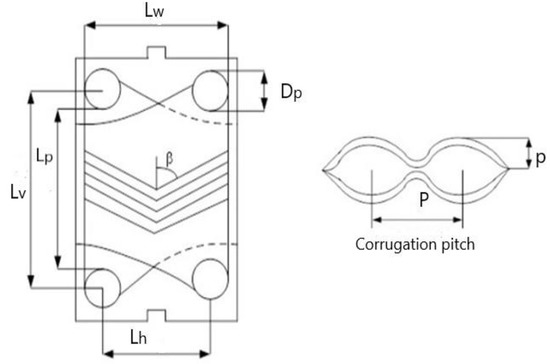
Figure 1. Main geometrical characteristics of a chevron corrugated plate.

The advantage to use large scale equipment for modeling is that models proceeding from laboratory scale experiments can be validated on it, on one hand, and newly developed models are more accurate, on the other hand.

Data collection was performed in a vegetable oil processing installation. It is a fully automated process. Temperatures are controlled at constant values by the cooling water flowrate in case of HE#2, HE#3, HE#4 and by the bleached oil flowrate in case of HE#1. Measured temperatures are shown in the third column of Table 2. The average temperature at the wall is calculated by considering no temperature gradient in it, so the temperature should be the same on both sides of the wall.

Table 2. The temperature of fluids.

HE #	Fluid	Temperature in (1) and out (2) of Hot (h) and Cold (c) Fluid, °C	Average Temperature of the Fluid, °C	Average Temperature at the Wall, °C
1	RO	$t_{c_1}=45;$$t_{c_2}=76$	60.5	69
	BO	$t_{h_1}=90$$; t_{h_2}=65$	77.5
2	RO	$t_{h_1}=85$$; t_{h_2}=42$	63.5	48.5
	Water	$t_{c_1}=30$$; t_{c_2}=37$	33.5
3	BO	$t_{h_1}=60$$; t_h=45$	52.5	42.7
	Water	$t_{c_1}=30$$; t_{c_2}=35.6$	32.8
4	WO	$t_{h_1}=110;$$t_{h_2}=40$	75	55
	Water	$t_{c_1}=30;$$t_{c_2}=40$	35

In each campaign, the measurements were performed during the steady-state regime which lasts for hours and days. In the case of first two campaigns, there were four such regimes when flowrates and temperatures remained constant. In the third campaign, the installation worked in only one steady-state regime.

2.2. Fluids

It is of great importance to determine the values of the physical properties of fluids with precision, either experimentally or by calculating with reliable mathematical correlations. Therefore, we determined, experimentally, the variation with temperature of density and dynamic viscosity of all three types of oils (raw, bleached, and winterised), covering the whole range in functioning (20–110 °C). The analyses were made with the apparatus Anton Paar, model SVM 3000 (Anton Paar OptoTech GmbH, Seelze-Letter, Germany), using the standard method ASTM D445/ISO 121852.

There were three processing campaigns in the factory, working with three crudes as follows: sunflower oil 1 (SO1), sunflower oil 2 (SO2) and rapeseed oil (RO).

By processing these data with the least squares’ method, the correlations allowing the calculation of oil density and viscosity at the working temperature were obtained. These correlations are given in Table 3 and Table 4.

Table 3. Mathematical correlation of vegetable oils density (g × cm⁻³) with temperature (°C).

Campaign/Oil	Oil Type	Equation	Coefficient of Determination, R2
I/SO1	RO	y = −0.0128 × x + 0.9308	0.9917
	BO	y = −0.0125 × x + 0.9296	0.9925
	WO	y = −0.0125 × x + 0.9296	0.9935
II/SO2	RO	y = −0.0122 × x + 0.9290	0.9905
	BO	y = −0.0126 × x + 0.9292	0.9935
	WO	y = −0.0124 × x + 0.9293	0.9903
III/RO	RO	y = −0.0125 × x + 0.9289	0.9937
	BO	y = −0.0124 × x + 0.9281	0.9907
	WO	y = −0.0126 × x + 0.9289	0.9929

Table 4. Mathematical correlation of vegetable oils viscosity (mPa × s) with temperature (°C).

Campaign/Oil	Oil Type	Equation	Coefficient of Determination, R2
I/SO1	RO	y = 68.283 × x−1.307	0.9959
	BO	y = 66.491 × x−1.277	0.9966
	WO	y = 68.338 × x−1.312	0.9958
II/SO2	RO	y = 65.051 × x−1.359	0.9991
	BO	y = 59.649 × x−1.226	0.9995
	WO	y = 66.409 × x−1.298	0.9958
III/RO	RO	y = 71.710 × x−1.325	0.9959
	BO	y = 68.285 × x−1.229	0.9964
	WO	y = 71.061 × x−1.322	0.9952

Even though the equations parameters seem very close for different type of oils, small differences can lead to bigger differences in similitude criteria values, especially for Prandtl numbers, with an effect on the accuracy of the mathematical model predicting the global heat transfer coefficients.

The specific heat capacity (c_p) and the thermal conductivity (λ) were estimated by the Equations (1) and (2) of Choi and Okos [24], developed for the vegetable oils:

$$c_p=1984.2+1473.3\times {10}^{-3}\times t-4800.8\times {10}^{-6}\times t^2 \left[\raisebox{1ex}{$\mathrm{J}$}\!\left/ \!\raisebox{-1ex}{$\mathrm{k}\mathrm{g}\times ℃$}\right.\right]$$

(1)

$$\lambda =0.18701-2.7604\times {10}^{-4}\times t-1.7749\times {10}^{-7}\times t^2 \left[\raisebox{1ex}{$\mathrm{W}$}\!\left/ \!\raisebox{-1ex}{$\mathrm{m}\times ℃$}\right.\right]$$

(2)

For cooling water, the physical properties at different temperatures (density, viscosity, specific heat capacity and thermal conductivity) are found in reference [25].

2.3. Modeling

The predominant heat transfer mechanism involved in this type of heat exchanger is the forced convection in stationary regime. Most correlations that are used for modeling the heat transfer describe the phenomenon in terms of similitude criteria, following the similitude theory, and the most frequent correlation is exponential (Equation (3)):

$$Nu=a\times R{e}^b\times P{r}^c$$

(3)

where: Nu, Re and Pr are three similitude criteria: Nusselt, Reynolds and Prandtl and coefficients a, b and c are to be determined for different flow regimes, for fluids with and without change in phase, for different geometries.

Reynolds number is calculated in relation to mass velocity in a channel G_ch [kg m⁻² s], hydraulic diameter d_h and dynamic viscosity μ (Equation (4)).

$$Re=\frac{G_{ch}\times d_h}{\mu }$$

(4)

Prandtl number is calculated from physical properties of the fluids with Equation (5).

$$Pr=\frac{c_p\times \mu }{\lambda }$$

(5)

Nu number contains the heat transfer coefficient α [W m⁻² °C⁻¹] which can be determined from Equation (6), after calculating Nu with Equation (3):

$$Nu=\frac{\alpha \times d_h}{\lambda }$$

(6)

For the forced convection in stationary regime, the coefficients a, b, c in Equation (3) were determined in many experimental studies but, the Kumar correlation (Equation (7)) is mostly recommended [18,26] to calculate Nu number when starting the development of a new and more accurate model.

$$Nu=0.348\times R{e}^{0.663}\times P{r}^{1/3}\times {\left(\frac{\mu }{{\mu }_w}\right)}^{0.17}$$

(7)

where μ_w is the dynamic viscosity of the fluid at the wall temperature.

The Equation (7) is valid when referring to the cross-sectional free area.

Lévêque gave another solution for the heat transfer during the laminar flow in the gap between two plates of length L and constant spacing H (Equation (8)), the so-called “1/3 power law”, confirmed by the numerical results of Holzbecher’s simulations [27]:

$$Nu=0.40377\times {\left(Re\times Pr\times \frac{H}{L}\right)}^{1/3}$$

(8)

The original Equation (8) was modified for micro-channels with sine ducts, after Martin [21] showed that the heat coefficient depends on pressure drop which is directly proportional to f_app × Re², where f_app is the apparent friction factor (Equation (9)):

$$N{u}_{sine}=0.40377\times {\left(4\times f_{app}R{e}_{sine}^2\times Pr\times \frac{d_{h,sine}}{L_{furr}}\right)}^{1/3}$$

(9)

Later, Dović and co-authors [22] adjusted this equation, taking into account the influence of factors ignored in the Equation (9) (swirling, real effective flow length), and in accordance with their own experimental data corroborated by other authors’ data [28,29] (Equation (10)):

$$N{u}_{sine}=0.38\times 0.40377\times {\left(4\times f_{app}R{e}_{sine}^2\times \frac{d_{h,sine}}{L_{furr}}\right)}^{0.375}P{r}^{1/3}{\left(\frac{\mu }{{\mu }_w}\right)}^{0.14}$$

(10)

In plate heat exchangers with chevron corrugations, the high heat transfer is due to the flow in small hydraulic diameter sections and interractions between streams flowing and generating swirl secondary flows. Dović and co-authors [22] describe the flow pattern, following an experiment with aqueous glycerol (62% wt.), with Re in range 0.1 to 250. This experiment allowed us to visualize two flow components: the furrow component (Equation (11)) and the longitudinal component (Equation (12)), and their partial mixing.

$$L_{furr}=\frac{l}{\sin \left(2\beta \right)}$$

(11)

$$L_{long}=p=\frac{l}{\sin \beta }$$

(12)

where l is the corrugation wavelength.

In the classical correlation (Equation (3)), Nu, Re and average velocity u [m/s] are related to the total chevron channel cross sectional area transverse to the main flow direction. Taking into account the sinusoidal flow, by means of analytical approach, the average velocity in the cell’s sine duct in furrow direction u_sine is recalculated with Equation (13):

$$u_{sine}=\frac{\dot{m_{ch}}}{\rho \times A_{ch, sine}}$$

(13)

where $\dot{m_{ch}}$ is the mass flowrate in the channel [kg/s], and $A_{ch, sine}$ is the channel cross-section transverse to the furrow (Equation (14)):

$$A_{ch, sine}=b\times L_W\times \cos \beta$$

(14)

L_w and β are geometrical characteristics from Table 1. Then, Reynolds sine is calculated with Equation (15).

$$R{e}_{sine}=\frac{u_{sine}{d}_{h,sine}}{\nu }$$

(15)

where d_h,sine is the the hydraulic diametre of a sine duct; it is related to the independent variable x—the ratio corrugation depth: corrugation wavelength (x = b/l), in Equation (16) [30]:

$$\frac{d_{h, sine}}{l}=0.1429x^3-0.623x^2+1.087x-0.0014$$

(16)

Nu_sine referred to the cell’s sine duct is correlated with Nu related to the the whole channel through Equation (17):

$$\frac{Nu}{N{u}_{sine}}=\frac{dh}{d{h}_{sine}}$$

(17)

L_furr in Equation (11) is the effective cell length L_cell, in case of β < 60°. In case of β > 60°, L_cell = L_long, following the prevailing pattern flow; f_app is the apparent friction coefficient which, for a given geometry, has the generalized form (Equation (18)):

$$f_{app}=\frac{C}{R{e}_{sine}}+B$$

(18)

Constants B (Equation (19)) and C (Equation (20)) are functions of channel geometry, and can be calculated as a function of the aspect ratio (x = b/l), by polynomial functions Equations (19)–(23), developed by Dović and co-authors [22] based on the work of Shah [30]:

$$B=\frac{K_{\infty }{d}_{h,sine}}{4\times L_{furr}}$$

(19)

$$C=2.6624x^4-10.586x^3+11.262x^2-0.1036x+9.6$$

(20)

$$K_e\left(\infty \right)=-5.888x^4+9.46113x^3-4.248x^2-0.1333x+2.648$$

(21)

$$K_d\left(\infty \right)=-1.7237x^4+2.7669x^3-1.2651x^2-0.0097x+1.512$$

(22)

$$K\left(\infty \right)=2\left[K_e\left(\infty \right)-K_d\left(\infty \right)\right]$$

(23)

where K$\left(\infty \right)$ represents the incremental pressure drop number, K_e-kinetic energy correction factor, and K_d is the momentum flux correction factor.

This model (Equations (10)–(23)) is intended to be validated by our own experimental data. The challenge is to find generalized correlations fitting to all flow regimes (laminar, intermediate and turbulent).

3. Results and Discussion

As mentioned before, there were three processing campaigns of vegetable oils. In two of them, the sunflower oils I and II were processed at four different flowrates, and in the third, the rapeseed oil was processed at one flowrate. In total, 72 sets of experimental data resulted. In Table 5, the total mass flowrate refers to the whole flowrate entering the circular port of the heat exchangers, since Re is calculated taking into account the hydraulic diameter of the channel, d_h (see also Table 1). The Nu number is calculated by applying the Kumar correlation (Equation (7)) from [18].

Table 5. Re, Nu and Pr criteria for chevron 30° channel related to cross sectional area transverse to the main flow direction.

Campaign	HE #	Fluids	Total Mass Flow Rate, kg/s	Re	Nu	Pr
Sunflower oil I ρ (20 °C) = 919.1 kg/m3 μ (20 °C) = 0.0662 Pa × s	1	RO	1.74/2.05/2.46/2.71	53/62/75/82	19.3/21.6/24.3/25.9	206.8
		BO	2.14/2.52/3.03/3.34	27/32/39/43	24.5/27.2/30.6/32.9	125.1
	2	RO	1.74/2.05/2.46/2.71	25/29/35/39	15.5/17.3/19.5/20.9	191.5
		Water	5.25/6.20/7.43/8.21	1546/1782/2154/2386	74.2/85.7/98.1/106.5	5.2
	3	BO	1.94/2.19/2.49/2.78	30/34/39/43	17.7/19.3/20.9/22.4	260.6
		Water	2.55/2.85/3.27/3.62	921/1038/1179/1305	58.4/63.3/68.9/73.7	5.3
	4	WO	1.74/2.05/2.46/2.71	18/21/26/28	11.7/12.8/14.4/15.3	135.8
		Water	6.02/7.11/8.52/9.41	979/1154/1379/1528	63.8/71.1/80.1/85.7	5.0
Sunflower oil II ρ (20 °C) = 918.1 kg/m3 μ (20 °C) = 0.0650 Pa × s	1	RO	1.74/2.05/2.46/2.71	58/68/81/90	20.3/22.7/25.6/27.3	170.7
		BO	2.14/2.52/3.03/3.34	33/39/47/52	24.2/27.0/30.5/32.6	136.6
	2	RO	1.74/2.05/2.46/2.71	29/35/42/46	16.6/18.6/20.9/22.4	160.1
		Water	5.25/6.20/7.43/8.21	1526/1801/2160/2385	74.5/86.0/98.4/107	5.2
	3	BO	1.94/2.19/2.49/2.78	25/28/32/35	19.1/20.7/22.6/24.1	213.6
		Water	2.55/2.85/3.27/3.62	919/1038/1179/1304	58.4/63.3/68.9/73.7	5.3
	4	WO	1.74/2.05/2.46/2.71	19/23/27/30	11.6/12.9/14.6/15.6	144.6
		Water	6.02/7.11/8.52/9.41	979/1156/1386/1530	63.8/71.2/80.3/85.9	5.0
Rapeseed oil ρ (20 °C) = 919.1 kg/m3 μ (20 °C) = 0.0694 Pa × s	1	RO	2.72	45	25.9	195.9
		BO	3.35	72	31.2	156.2
	2	RO	2.72	40	21.4	184.4
		Water	8.23	2391	112.6	5.2
	3	BO	2.76	38	23.0	244.0
		Water	3.62	1306	73.7	5.3
	4	WO	2.72	27	15.3	149.6
		Water	9.44	1533	85.9	5.0

As seen in Table 5, the experimental data covers a range of laminar flow regime (Re = 18–90, Re < 100) and another range of fully developed turbulent regime (Re = 921–2391, Re > 250). Re and Nu numbers, related to the chevron channel cross sectional area transverse to the main flow direction, served later to calculate the experimental values of Re_sine and Nu_sine, related to cell’s sine duct in furrow direction.

Both Equations (9) and (10) consider that heat transfer depends on pressure drop, which is directly proportional to product fRe². Additionally, u_sine, dh_sine, f_app, L_furr, and constants B and C were determined in each experimental point, for the Nu_sine,calc estimation, according to the model of Lévêque adjusted by Dović et al. [22].

The constants B and C were calculated with Equations (18)–(23), for each heat exchanger and the average values were B = 0.19952 ± 0.00006 and C = 12.4239 ± 0.0121. These values are for the first time calculated in case of gasket plate heat exchangers with corrugation angles 30° and the aspect ratio b/l = 0.8, since the model to be validated recommends application for b/l < 0.5.

The friction factor, f_app, determined in each experimental point with Equation (17), was plotted vs. Re_sine (Figure 2) and compared with the model, on the whole range of Re_sine = 8–1137. The model fits almost perfectly at Re_sine > 25 with experimental data of Muley et al. [13] and Heavner [31] but has errors of 5–15% at Re_sine = 9–25. These errors can be explained by the different geometry (the aspect ratio b/l > 0.5 in contrast with b/l < 0.5 for all previous experiments), which can affect the friction coefficients at Re sine < 25.

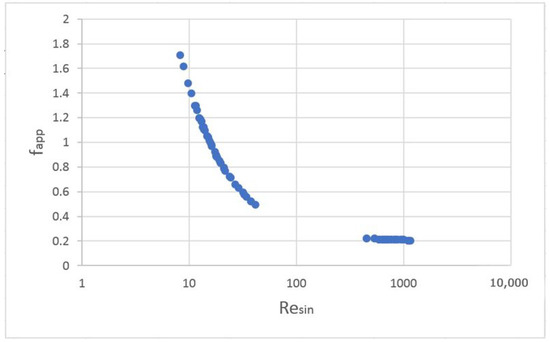
Figure 2. Variation of apparent friction coefficients (f_app) with Re_sine in the present experiment.

Since Re numbers are between 18 and 2391, Re_sine are between 8 and 1137. Moreover, Nu numbers related to the main flow direction, calculated with Kumar correlation are between 6.1 and 112.6, since Nu_sine,exp values related to the sine duct flow are between 4.5 and 42.2. These similitude criteria together with Nu_sine,calc, calculated with model Equations (9)–(23) are shown in Table 6. This table also includes the relative errors between the experimental values of Nu_sin,exp (Equation (14)) and those computed with adjusted correlation Lévêque (Equation (10)).

Table 6. Re_sine, Nu_sine,exp and Nu_sine,calc related to the sine duct flow, for corrugation inclination angle 30°.

HE #	Fluids	Total Massflow Rate, kg/s	Resine	Nusine,exp	Nusine,calc	Relative Error, %
Sunflower oil I ρ (20 °C) = 919.1 kg/m3, μ (20 °C) = 1.0662 Pa × s
1	RO	1.74/2.05/2.46/2.71	13/15/18/20	7.6/8.5/9.6/10.2	8.5/9.1/9.9/10.4	10.0/6.3/3.2/1.4
	BO	2.14/2.52/3.03/3.34	27/31/38/42	9.7/10.8/12.1/13.0	9.4/10.2/11.2/11.8	−2.8/−5.3/−7.9/−10.1
2	RO	1.74/2.05/2.46/2.71	11/13/16/18	6.1/6.8/7.7/8.2	7.1/7.7/8.3/8.7	14.4/11.3/7.8/5.5
	Water	5.25/6.20/7.43/8.21	701/808/977/1082	29.3/33.8/38.7/42.0	27.5/30.5/35.0/37.7	−6.3/−10.7/−10.4/−11.3
3	BO	1.94/2.19/2.49/2.78	11/13/15/15	7.0/7.6/7.9/8.3	6.7/7.1/7.4/7.4	−5.0/−8.5/−5.7/−11.5
	Water	2.55/2.85/3.27/3.62	586/661/752/854	23.1/25.0/27.2/29.1	23.9/26.0/28.5/31.2	3.2/3.8/4.5/6.8
4	WO	1.74/2.05/2.46/2.71	9/10/12/14	4.6/5.1/5.7/6.0	5.6/6.0/6.5/6.8	17.4/15.7/12.4/10.9
	Water	6.02/7.11/8.52/9.41	446/525/628/696	24.0/27.0/30.5/32.6	20.3/22.8/25.9/27.9	−18.2/−18.1/−17.8/−17.1
Sunflower oil II ρ (20 °C) = 918.1 kg/m3, μ (20 °C) = 0.0650 Pa × s
1	RO	1.74/2.05/2.46/2.71	15/18/21/24	7.6/8.5/10.1/10.8	8.4/9.1/9.9/10.4	4.7/ 1.0/−2.3/−4.2
	BO	2.14/2.52/3.03/3.34	24/28/34/38	9.6/10.7/12.0/12.9	9.3/10.0/11.0/11.6	−3.3/−6.5/−9.8/−11.5
2	RO	1.74/2.05/2.46/2.71	13/16/19/21	6.5/7.3/8.2/8.8	7.2/7.8/8.5/8.9	9.3/5.9/2.6/0.3
	Water	5.25/6.20/7.43/8.21	694/820.981/1085	29.6/33.9/38.3/42.2	27.2/30.7/34.9/37.0	−8.0/−10.6/−11.0/−13.3
3	BO	1.94/2.19/2.49/2.78	14/16/18/20	7.5/8.2/8.9/9.5	8.2/8.6/9.2/9.6	8.0/5.4/2.6/0.9
	Water	2.55/2.85/3.27/3.62	586/661/752/854	23.1/25.0/27.2/29.1	23.7/25.8/28.3/31.0	2.6/3.2/4.0/6.3
4	WO	1.74/2.05/2.46/2.71	8/10/12/13	4.6/5.1/5.8/6.2	6.4/6.9/7.4/7.8	28.5/25.9/22.5/20.6
	Water	6.02/7.11/8.52/9.41	446/528/633/698	24.0/26.9/30.5/32.6	20.2/22.7/22.9/31.0	−18.8/−18.3/17.8/−17.5
Rapeseed oil I ρ (20 °C) = 919.5 kg/m3, μ (20 °C) = 0.0694 Pa × s
1	RO	2.72	21	10.2	10.3	1.1
	BO	3.35	32	12.3	11.4	−8.2
2	RO	2.72	18	8.4	8.8	4.8
	Water	8.23	1137	32.3	28.2	14.7
3	BO	2.76	17	9.1	9.6	5.5
	Water	3.62	923	29.1	33.0	11.9
4	WO	2.72	12	6.1	6.9	12.5
	Water	9.44	700	33.9	28	−21.1

For the whole set of data, the relative errors are between −18.8% and +28.5%, both positive and negative values, demonstrating that they are not systematical errors. The medium error is $\left|\overline{\epsilon }\right|$ = 9.56%.

The plot Nu_sine,calc vs. Nu_sine,exp (Figure 3), showing the dispersal of data around the bisector, uncovers that points spreading is minimal at lower values of Nu_sine, corresponding to the laminar flow, since at values corresponding to the turbulent flow, Nu_sine are spread at a bigger distance; however, dispersal on both sides of the bisector for these values too, indicates that the model can be used up to Re_sine = 1137, with confidence.

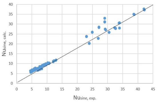
Figure 3. Comparison between the experimental Nu_sine values and those computed with the model (Equation (10)).

For the forced convection in stationary regime, it is customary to look for corelations between Re and Nu/Pr^1/3 (μ/μ_w)^0.14. We used the facility Data analysis in Excel. The computed results for the similitude criteria taking into account the sine duct flow are shown in Table 7.

Table 7. Statistical data analysis for Re_sine vs. Nu_sine /Pr^1/3 (μ/μ_w)^0.14 correlation.

SUMMARY OUTPUT
Regression Statistics
Multiple R	0.9924
R Square	0.9849
Adjusted R Square	0.9847
Standard Error	0.9093
Observations	72
ANOVA
	df	SS	MS	F	Significance F
Regression (treatments)	1	3770.1214	3770.1214	4559.34	1.85 × 10−65
Residual (errors)	70	57.8830	0.8269
Total	71	3828.0
	Coefficients	Standard Error	t Stat	p-value	Lower 95%	Upper 95%
Intercept	1.3305	0.1364	9.75	1.11 × 10−14	1.0585	1.6026
X Variable 1	0.0195	0.0003	67.52	1.85 × 10−65	0.0189	0.0201

As seen in Table 7, both regression statistics and ANOVA analysis show that Re_sine and Nu_sine/Pr^1/3 (μ/μ_w)^0.14 are strongly correlated through linearity. The coefficient of determination is close to 1 (R² = 0.9849). The ANOVA variance test demonstrated that null hypothesis is false, so the mean squares for treatments MST is much larger than the mean squares for errors MSE (3770.1214 $\gg$0.8269); the MST/MSE ratio is F = 4559.34, a very high value, far from F = 1, the value for non-correlated series of data. In conclusion, the Fisher test confirms the strong correlation between the series of data. The linear correlation (Equation (24)):

Nu_sine/Pr × (μ/μ_w)^0.14 = 1.3305 + 0.0195 Re_sine

(24)

The p-values $<$ 0.05 for the intercept and the slope of the line demonstrate that the model works with the confidence in the interval ±95%. Nu_sine includes the partial heat transfer coefficient α in the fluid on one side of the plate; the coefficient on the other side of the plate can be calculated with the corresponding value of Nu_sine. Taking also into account the conductivity of the plate material, the overall heat transfer coefficient can be found. It is very important to have an accurate model for the estimation of Nu_sine, because the errors spread in the values of the overall coefficient.

4. Conclusions

In this study, the semi-analytical model of Lévêque for heat transfer in gasket plate heat exchanger channels was validated in our experimental data obtained from industrial equipment for vegetable oil processing. The vegetable oils had different physical properties proceeding from three different raw materials in different stages of the process (raw, bleached, winterized). There were four exchangers with similar geometry but different in size. The flow regime was laminar (Re < 100) for oils and turbulent (Re > 250) for water, allowing us to check the model in a large range of Re numbers, related to the cross-sectional free area of the channel.

The model of Lévêque takes into consideration the flow in cell’s sine duct in furrow direction. Consequently, the similitude criteria Re_sine and Nu_sine are calculated in new considered conditions. They are correlated with a more complex relationship, considering the construction details of the channels. In this work, the constants C and D of the model were determined, for corrugation inclination angle relative to vertical direction equal to 30°, for the first time. Thus, B = 0.19952 ± 0.00006 and C = 12.4239 ± 0.0121. As regards the constant C₁ of the model, that is the same as determined by Dović et al. [22] when adapting Lévêque correlation to the corrugation inclination angle 60° (C₁ = 0.1534).

Both the analysis of relative errors and the statistical analysis concluded that Lévêque correlation adapted by Dović et al., with model parameters, determined here for corrugation angle 30°, can be used with confidence for predicting Nu criterium as a basis for heat transfer calculations in gasket plate exchangers.

References

- Han, D.-H.; Lee, K.-J.; Kim, Y.-H. The caracteristics of condensation in brazed plate heat exchangers with different chevron angles. J. Korean Phys. Soc. 2003, 43, 66–73. [Google Scholar]
- Nikhil, G.J.; Shailendra, M.L. Heat Transfer Analysis of Corrugated Plate Heat Exchanger of Different Plate Geometry: A review. Int. J. Emerg. Technol. Adv. Eng. 2012, 2, 110–115. [Google Scholar]
- Jin, S.; Hrnjak, P. Effect of end plates on heat transfer of plate heat exchanger. Int. J. Heat Mass Transf. 2017, 108, 740–748. [Google Scholar] [CrossRef] [Green Version]
- Yang, J.; Jacobi, A.; Liu, W. Heat transfer correlations for single-phase flow in plate heat exchangers based on experimental data. Appl. Therm. Eng. 2017, 113, 1547–1557. [Google Scholar] [CrossRef]
- Gulenoglu, G.; Akturk, F.; Aradag, S.; Uzol, N.S.; Kakaci, S. Experimental comparison of performances of three different plates for gasketed plate heat exchangers. Int. J. Therm.Sci. 2014, 75, 249–256. [Google Scholar] [CrossRef]
- Yildiz, A.; Ersoz, M.A. Theoretical and experimental thermodynamic analyses of a chevron type heat exchanger. Renew. Sustain. Energ. Rev. 2015, 42, 240–253. [Google Scholar] [CrossRef]
- Hu, Z.; He, X.; Ye, L.; Yang, M.; Qin, G. Full-scale research on heat transfer and pressure drop of high flux plate heat exchanger. Appl. Therm. Eng. 2017, 118, 585–592. [Google Scholar] [CrossRef]
- Eimaaty, T.M.A.; Kabeel, A.E.; Mahgoub, M. Corrugated plate heat exchanger review. Renew. Sust. Energ. Rev. 2017, 70, 852–860. [Google Scholar] [CrossRef]
- Bobbili, P.R.; Sunden, B.; Das, S.K. An experimental investigation of the port flow maldistribution in small and large plate package heat exchangers. Appl. Therm. Eng. 2006, 26, 1919–1926. [Google Scholar] [CrossRef]
- Wang, L.; Sunden, B. Optimal design of plate heat exchangers with and without pressure drop specifications. Appl. Therm. Eng. 2003, 23, 295–311. [Google Scholar] [CrossRef]
- Gut, J.A.W.; Pinto, J.M. Modeling of Plate Heat Exchangers with Generalized Configurations. Int. J. Heat Mass Transf. 2003, 46, 2571–2585. [Google Scholar] [CrossRef]
- Al-Zahrani, S.; Islam, M.S.; Saha, S.C. Comparison of flow resistance and port maldistribution between novel and conventional plate heat exchangers. Int. Comm. Heat Mass Transf. 2021, 123, 105200. [Google Scholar] [CrossRef]
- Muley, A.; Manglik, R.M. Experimental study of turbulent flow heat transfer and pressure drop in a plate heat exchanger. ASME J. Heat Transf. 1999, 121, 110–117. [Google Scholar] [CrossRef]
- Wanniarachchi, A.S.; Ratnam, U.; Tilton, B.E.; Dutta-Roy, K. Approximate Correlations for Chevron-Type Plate Heat Exchangers. In Proceedings of the ASME National Heat Transfer Conference, Portland, OR, USA, 5–9 August 1995; Volume 314, pp. 145–151. [Google Scholar]
- Warnakulasuriya, F.S.K.; Worek, W.M. Heat transfer and pressure drop properties of high viscous solutions in plate heat exchangers. Int. J. Heat Mass Transf. 2008, 51, 52–67. [Google Scholar] [CrossRef]
- Naik, V.R.; Matawala, V.K. Experimental Investigation of Single Phase Chevron Type Gasket Plate Heat Exchanger. Int. J. Eng. Adv. Technol. 2013, 2, 362–369. [Google Scholar]
- Akturk, F.; Gulben, G.; Aradag, S.; Uzol, N.S.; Kakac, S. Experimental Investigation of the Characteristics of a Chevron Type Gasketed-Plate Heat Exchanger. In Proceedings of the 6th International Advanced Technologies Symposium (IATS’11), Elazig, Turkey, 16–18 May 2011. [Google Scholar]
- Kakac, S.; Liu, H. Heat Exchangers. Selection, Rating and Thermal Design, 2nd ed.; CRC Press: Boca Raton, FL, USA, 2002. [Google Scholar]
- Zhong, Y.; Deng, K.; Zhao, S.; Hu, J.; Zhong, Y.; Li, Q.; Wu, Z.; Lu, Z.H.; Wen, Q. Experimental and Numerical Study on Hydraulic Performance of Chevron Brazed Plate Heat Exchanger at Low Reynolds Number. Processes 2020, 8, 1076. [Google Scholar] [CrossRef]
- Arsenyeva, O.; Tovazhnyansky, L.; Kapustenko, P.; Khavin, G. Mathematical Modelling and Optimal Design of Plate-and-Frame Heat Exchangers. Chem. Eng. Trans. 2009, 18, 791–796. [Google Scholar] [CrossRef]
- Martin, H. A theoretical approach to predict the performance of chevron-type plate heat exchangers. Chem. Eng. Process Process. Intensif. 1996, 35, 301–310. [Google Scholar] [CrossRef]
- Dović, D.; Palm, B.; Švaić, S. Generalized correlations for predicting heat transfer and pressure drop in plate heat exchanger channels of arbitrary geometry. Int. J. Heat Mass Transf. 2009, 52, 4553–4563. [Google Scholar] [CrossRef]
- Piper, M.; Zibart, A.; Kenig, E.Y. New design equations for turbulent forced convection heat transfer and pressure loss in pillow-plate channels. Int. J. Sci. 2017, 120, 459–468. [Google Scholar] [CrossRef]
- Oniţă, N.; Ivan, E. Calculations in the Food Industry. Handbook (Memorator Pentru Calcule în Industria Alimentară); Mirton: Timişoara, Romania, 2006. (In Romanian) [Google Scholar]
- Ražnjević, K. Handbook of Thermodynamic Tables and Charts; Hemisphere Pub. Corp.: Washington, DC, USA, 1976. [Google Scholar]
- Neagu, A.A.; Koncsag, C.I.; Barbulescu, A.; Botez, E. Calculation methods for gasket plate heat exchangers used in vegetable oil manufacture. Comp. Study Rev. Chim. 2015, 66, 1504–1508. [Google Scholar]
- Holzbecher, E. Numerical Solutions for the Lévêque Problem of Boundary Layer Mass or Heat Flux. In Proceedings of the European COMSOL Conference, Hannover, Germany, 4–6 November 2008; Available online: https://www.comsol.ch/paper/download/37491/Holzbecher.pdf (accessed on 20 December 2021).
- Muley, A.; Manglik, R.M.; Metwally, H.M. Enhanced heat transfer characteristics of viscous liquid flows in a chevron plate heat exchanger. ASME J. Heat Transf. 1999, 121, 1011–1017. [Google Scholar] [CrossRef]
- Okada, K.; Ono, M.; Tomimura, T.; Okuma, T.; Konno, H.; Ohtani, S. Design and heat transfer characteristics of new plate heat exchanger. Heat Trans. Jpn. Res. 1972, 1, 90–95. [Google Scholar]
- Shah, R.K. Laminar flow friction and forced convection heat transfer in ducts of arbitrary geometry. Int. J. Heat Mass Transf. 1975, 18, 849–862. [Google Scholar] [CrossRef]
- Heavner, R.L.; Kumar, H.; Wanniarachchi, A.S. Performance of an Industrial Plate Heat Exchanger: Effect of Chevron Angle. AIChE Symposium Series; American Institute of Chemical Engineers: New York, NY, USA, 1993; Volume 89, pp. 262–267. [Google Scholar]
Publisher’s Note: MDPI stays neutral with regard to jurisdictional claims in published maps and institutional affiliations. |
© 2022 by the authors. Licensee MDPI, Basel, Switzerland. This article is an open access article distributed under the terms and conditions of the Creative Commons Attribution (CC BY) license (https://creativecommons.org/licenses/by/4.0/).