Statistical Deadband: A Novel Approach for Event-Based Data Reporting

Abstract

Deadband algorithms are implemented inside industrial gateways to reduce the volume of data sent across different networks. By tuning the deadband sampling resolution by a preset interval $\Delta$, it is possible to estimate the balance between the traffic rates of networks connected by industrial SCADA gateways. This work describes the design and implementation of two original deadband algorithms based on statistical concepts derived by John Bollinger in his financial technical analysis. The statistical algorithms proposed do not require the setup of a preset interval—this is required by non-statistical algorithms. All algorithms were evaluated and compared by computing the effectiveness and fidelity over a public collection of random pseudo-periodic signals. The overall performance measured in the simulations showed better results, in terms of effectiveness and fidelity, for the statistical algorithms, while the measured computing resources were not as efficient as for the non-statistical deadband algorithms.

1. Introduction

Statistical methods in manufacturing procedures for quality control were investigated by Friedman [1]. The statistical and temporal properties of crossings at a certain level by random signals in manufacturing process control were first with the send-on-delta sampling scheme by Ellis [2,3]. However, in manufacturing supervision and control networks, more attention is given to the volume of data generated by the messages than to the power and computing resources required to send them [4]. The first OPC (OLE technology for process control) standard [5], established at the beginning of 1990s, was the OPC deadband, which is a send-on-delta sampling schema for data-reporting algorithms in industrial gateways, used to reduce the volume of data sent from the fieldbus (networks of devices such as transmitters and actuators) to the SCADA (supervisory control and data acquisition) network layer in a manufacturing environment. Variants of the same algorithm have been introduced by the NI LabView tool [6] and Lonworks technology [7]. The absolute deadband (AD) schema is known in the signal processing literature as conventional send-on-delta (SoD) in order to differentiate it from the other algorithm variants [8]. It is considered deterministic because it requires a preset interval of oscillations where the signal should be limited a priori.

The SoD schema is a natural, signal-dependent, temporal, event-based data report schema, while Bollinger’s financial theory can be considered as a signal-independent prediction schema [9].

Using the deadband concept, a continuous time signal $y\left(t\right)$ is sampled and a new report is sent when the value of the physical variable being sensed deviates from the value included in the most recent report by a preset interval, $\pm \Delta$, where $\Delta >0$. Using the statistical approach, a new report is sent when the value of the physical variable being sensed deviates from the value included in the most recent report by a non-related statistical indicator with a preset interval $\Delta$.

The objective of this work is to implement statistical algorithms based on Bollinger’s theory as alternatives to the conventional SoD sampling scheme, which is an event-based data-reporting strategy.

The experimental results showed a performance enhancement of the statistical deadband algorithms over the non-statistical send-on-delta schema. In order to reproduce the algorithms comparison in R [10], the pseudo-code of all of the algorithms in this paper have a corresponding function in the deadband package [11]. The algorithms described in the pseudo-code represent the concept to obtain the algorithm output, sample by sample, as in the online working mode. The corresponding functions in the package process the collection of all outputs for all input samples in a finite time period. The functions in the package have been developed to compare the overall performance of a hypothetical device that embeds a hardware or software implementation of the corresponding pseudo-code algorithms.

This paper is organized as follows. Section 2 presents an introduction to the OPC deadband concepts that are related to the data collection process and the algorithms. Section 3 presents Bollinger’s technical analysis. Section 4 presents the two original deadband algorithms. Section 5 provides the simulation results developed by using the deadband package. Finally, Section 6 draws some conclusions.

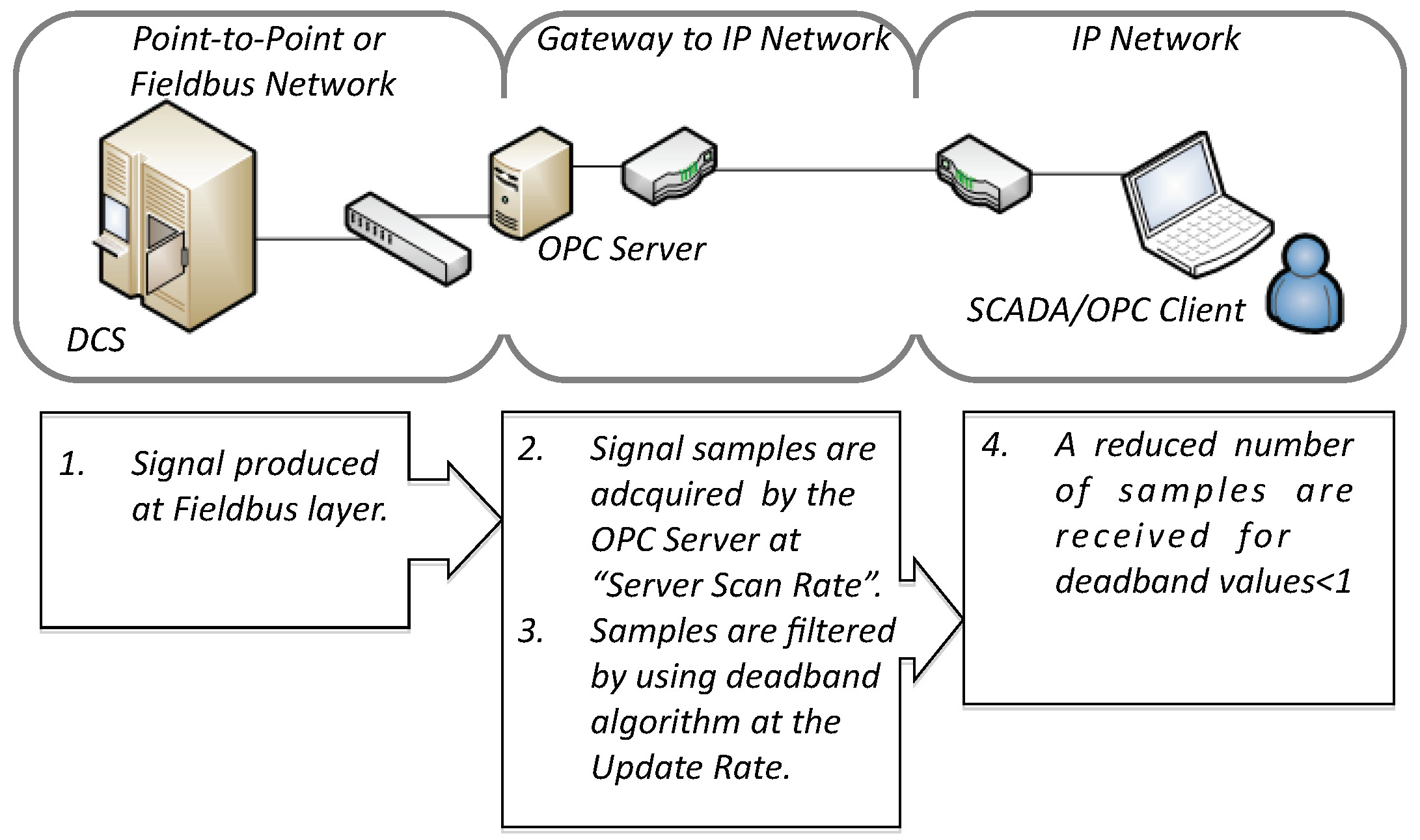
2. OPC Deadband and Event-Based Reporting Strategy

In sensors literature, the absolute deadband algorithm is explored as an SoD event-based control problem and usually makes the prior assumption that an event generator is established in advance. Then suitable control laws are calculated in order to ensure the stability of the original system [3].

In sensor networks literature, [12] SoD event-based approaches are proposed in order to provide a trade-off between the effectiveness and resource utilization/energy efficiency. Diaz et al., in Reference [13], introduced a dynamic SoD by using a network adaptive scheme over network transport protocols for remote controlled sensors. Hirche et al., in Reference [14], introduced the concept of a relative SoD by adding a proportional factor to $\Delta$ of the conventional deadband, according to the amplitude of the signal. Suh, in Reference [15], proposed the addition of a linear predictor in the conventional SoD reconstructor schema, in order to reduce the number of samples transmitted. After a sensor value transmission, a linear predictor computes the future sensor value based on the past values. If the difference between the current value and the predicted value is larger than a prefixed $\Delta$, the sensor value is transmitted.

The main objective of an event-based reporting strategy is to avoid sampling periodically and rather only sample when a quantized data change occurs, from one possible value to the next. The OPC standard, set by the OPC Foundation^®, extends the data report schema to networks in order to open software application interoperability between automation and control applications, field device applications controller (such as Proportional–Integral–Derivative—PID or sensors), and office applications [16]. The basic principle of OPC operation is that an OPC client, a SCADA software for example, transfers data to/receives data from fieldbus devices by using an industrial gateway, named the OPC server. The OPC client can operate either locally, or via a local or remote network. In this case the server accesses field devices via drivers.

In order to explain how the OPC deadband algorithm reports the data from the fieldbus (left side) to the networks (right side), as outlined in Figure 1, we consider a sampled signal $y\left(t\right)$ at the OPC server, originating from a field device connected to the OPC server using a dedicated hardware and software library. The first step in Figure 1 is the generation of the signal at the field device or a DCS (distributed control system). Then, samples of $y\left(t\right)$ are acquired at the OPC server, which reports to the OPC client. The sensed samples are those that deviate from the values included in the most recent report, called the cache ($y_{cache}\left(t\right)$). From the fieldbus side, we assume the physical sampling rate of $y\left(t\right)$, is established and pre-configured by the field technology vendor. This sampling rate is represented by the parameter $ServerScanRate$ in the OPC server and determined by using the field device vendor library [17,18]. From the SCADA/OPC client side, the reported changes of $y\left(t\right)$ are received at an update rate negotiated by the OPC server and client—the OPC client requests the subscription to changes by the $RequestedUpdateRate$ parameter and the OPC server responds by the $RevisedUpdateRate$, either by accepting the proposed rate or, if it is too high, by downgrading the rate to the $ServerScanRate$. In most cases, the $ServerScanRate$ is a physically bounded value in the field device and is also specified inside the OPC server device driver.

The deadband algorithm is applied by the OPC server to the sampled signals $y\left(t\right)$ to determine which one may be reported to the OPC client at the update rate. According to the send-on-delta (SoD) schema, it can skip the samples that do not representing relevant changes for the OPC client. At reception, the OPC client uses the zero-order hold (ZOH) strategy, where the last received data are held at the SCADA application until new data arrive. Therefore, the missing data are estimated by holding the value of the last received sample.

The OPC clients are used to monitor and control client/server network applications, the deadband algorithm parameter is tuned in order to minimize the amount of data sent from the OPC server to the client [19,20,21,22]. The number of requests and responses in the supervision network can increase exponentially with a high frequency of samples sent by the gateway [23]. For such a reason, the OPC client has to indicate that the amount of data being sensed deviates from the value included in the most recent report by using a parameter called the deadband percentage, or d, which is defined as the percentage that a relevant value must change by before the value is out of the client’s interest. Changes in values out of the client’s interest are not sent, reducing the amount of data delivered over the network.

The Absolute Deadband Algorithm

The absolute deadband (AD) algorithm, known also as constant deadband in sensors literature [14], is applied to each new sample $y\left(t\right)$ provided by the OPC server at the update rate. First, the gateway computes the interval $\Delta$ using the deadband parameter d as expressed by Equation (1):

$$\Delta =(E{U}_{max}-E{U}_{min})d0\le d\le 1,$$

(1)

where d is the deadband percentage; and $E{U}_{min}$ and $E{U}_{max}$ are the lower and upper bounds of an analog signal previously calibrated for some phenomena and typed in the device description [24,25]. The difference $(E{U}_{max}-E{U}_{min})$ is the preset interval. For example, considering a thermometer for the human body, these values are typically bounded from 35 to 42 degrees Celsius, representing the preset interval for a limited temperature range, known a priori.

As a second step, the gateway verifies the sampling deadband equation, also known as the absolute deadband (AD) equation. In other engineering control applications, this is also known as the trigger-function or amplitude-sensitive equation [26,27,28]. Given a sampled signal $y\left(t\right)$ at $t=t^{\ast }$, it is defined as:

$$|y_{t^{\ast }}-y_{t_{cache}}|>\Delta .$$

(2)

In Equation (2), $y_{t^{\ast }}$ represents the current sample value at the update rate and $y_{t_{cache}}$ is the last data report sent by the algorithm to the remote SCADA/OPC client and saved in cache memory.

The device implementing the AD algorithm, as summerized in Algorithm 1, verifies, sample by sample, each new value of the Equation (2) to decide whether the current sample value is out of the client’s interest or has to be reported.

The OPC deadband algorithm is the absolute deadband algorithm combined with a network strategy report, which is found in most industrial communication systems, such as the OPC-XML advanced polling and publisher/subscriber approach technology, OPC 2.x/3.x, OPC-UA, Lonworks, and the NI LabView standards [5].

Algorithm 1 Absolute Deadband (AD)
procedure Absolute Deadband ($E{U}_{min}$, $E{U}_{max}$, $y_{t^{\ast }}$, $y_{t_{cache}}$, d)
$\Delta \leftarrow (E{U}_{max}-E{U}_{min})·d$
if $|y_{t^{\ast }}-y_{t_{cache}}|>\Delta$ then
send $y_{t^{\ast }}$	▹ Signal will be sent
$y_{t_{cache}}\leftarrow y_{t^{\ast }}$	▹ Update the last recorded signal
else
discard $y_{t^{\ast }}$
end if
end procedure

3. The Bollinger Financial Technical Analysis

In 1983, John Bollinger introduced a set of technical analysis tools for the financial market named Bollinger Bands ™. The key of Bollinger Bands is the price volatility represented in the Bollinger formulas by the standard deviation $\sigma$ and the moving average. Financial traders use the outputs of Bollinger Bands with other technical indicators in order to predict the future price and choose the position to take with regard to the monitored asset. The indicators work with time series of stock market closing prices over periods of 10, 20, and 50 days.

In the case of industrial monitoring, we have a time series representing the samples of $y\left(t\right)$. For each $t=t^{\ast }$, Equation (3) defines the moving average ($mave$) of a time series $y\left(t\right)$ over n periods:

$$mav{e}_{t^{\ast }}=\sum _{t=t^{\ast }-n+1}^{t=t^{\ast }}{y}_t/n.$$

(3)

Since, in Equation (3), the moving average uses n data values, the first time $t^{\ast }$ at which $mav{e}_{t^{\ast }}$ can be calculated is $t^{\ast }=n$. For this reason, the adaptation of Bollinger’s theory to a sampled signal is applicable after the acquisition of n consecutive samples. Similarly, let n be the period of variance at $t=t^{\ast }$; then ${\sigma }_{t^{\ast }}^2$ is defined as:

$${\sigma }_{t^{\ast }}^2=\sum _{t=t^{\ast }-n+1}^{t=t^{\ast }}{(y_t-mav{e}_{t^{\ast }})}^2/(n-1).$$

(4)

The band components are constructed using a center line and an upper and lower band, defined respectively as:

$$centerlineB{B}_{t^{\ast }}=mav{e}_{t^{\ast }}$$

(5)

$$upperB{B}_{t^{\ast }}=mav{e}_{t^{\ast }}+k\ast {\sigma }_{t^{\ast }}$$

(6)

$$lowerB{B}_{t^{\ast }}=mav{e}_{t^{\ast }}-k\ast {\sigma }_{t^{\ast }}.$$

(7)

The parameter k is a width multiplier and represents the distance, in units of standard deviations, from the center line to each band. In stock market financial analysis, Reference [29] recommends the n and k values shown in

Table 1. Recommended Width Parameters for Bollinger Bands.

Periods (n)	Multiplier (k)
10	1.9
20	2.0
50	2.1

for bands construction.

While, in finance, n represents the number of days spent on price observations, in engineering applications, the period n may represent other temporal unit scales and the required observations could be more than fifty. Instead of number of days, in this study, n is considered a time sequence of consecutive samples at the OPC server.

In Bollinger technical analysis, the values of $k=2$ and $n=20$ are considered as a reference case and the other combinations are used to expand the reference case. In Reference [30], the Bollinger bands are used to detect defections in patterned fabric and the reference values of n and k were 20 and 2, respectively. For most financial analyses, the default choice for the average is a simple moving average, but other types of averages can be employed as needed [31].

For each $y\left(t^{\ast }\right)$ with $t^{\ast }>n$, the Bollinger theory introduces two indicators derived directly from the bands:

$$\%B_{t^{\ast }}=\frac{y_{t^{\ast }}-lowerB{B}_{t^{\ast }}}{upperB{B}_{t^{\ast }}-lowerB{B}_{t^{\ast }}}.$$

(8)

As defined in Equation (8), the volatility indicator, $\%B_{t^{\ast }}$, measures the relative proximity of the sample value to the previous period. It typically varies from 0 to 1, but it can occasionally exceed these values: when the value of $\%B$ trends to 1, the value moves to the upper band; and when $\%B$ trends to 0, the value moves to the lower band.

The second indicator, called the BandWidth, is defined in Equation (9):

$$BandWidt{h}_{t^{\ast }}=\frac{upperB{B}_{t^{\ast }}-lowerB{B}_{t^{\ast }}}{centerlineB{B}_{t^{\ast }}}.$$

(9)

It is used to recognize the beginning and end of increasing and decreasing values. Both parameters can also be used together to recognize trend patterns.

4. Bollinger Deadband and Volatility Deadband Algorithms

In this section, we propose the Bollinger deadband and the volatility deadband algorithms. The first algorithm, described in Section 4.1, performs the same logic as the absolute deadband (AD) approach but assumes the preset interval is the range between the upper and lower bands of the Bollinger theory. For this reason, it was named the Bollinger deadband (BD). The second algorithm, detailed in Section 4.2, does not use the bands and does not calculate any $\Delta$. It compares the volatility indicator, $\%B$, to the deadband percentage parameter, d, and discards the sample if the indicator is less than or equal to the percentage deadband. For this reason, it was named the volatility deadband (VD) approach.

Since both algorithms, BD and VD, require n consecutive samples at the beginning of algorithm in order to calculate the moving average, no samples are reported until after the n-th sample.

4.1. Bollinger Deadband: An Algorithm Using the Upper and Lower Bands

For a sample of $y\left(t\right)$ at $t=t^{\ast }$, the algorithm computes $\Delta$ as in Equation (10):

$${\Delta }_{t^{\ast }}=(upperB{B}_{t^{\ast }}-lowerB{B}_{t^{\ast }})d0\le d\le 1.$$

(10)

Let ${\mathbf{y}}_n\left(t\right)$ be a vector of n consecutive samples sent by any sensor or device to the OPC server. Its size is the same as the number of periods adopted to compute the upper and lower bands. Let k be the multiplier in Bollinger’s theory and d be a real number representing the deadband percentage. For each new value of the series ${\mathbf{y}}_n\left(t\right)$ at $t=t^{\ast }$, the proposed Bollinger deadband algorithm computes the SoD sampling schema assuming $\Delta$ as in Equation (10). This is described in the pseudo-code presented in Algorithm 2.

Algorithm 2 Bollinger Deadband (BD)
procedure Bollinger Deadband ($y_{t^{\ast }}$, ${\mathbf{y}}_n\left(t\right)$, n, k, d, $y_{t_{cache}}$)
if ${\mathbf{y}}_n\left(t\right)<n$ then	▹ No filter for the first n periods
${\mathbf{y}}_t\left(n\right).Enqueue\left(y_{t^{\ast }}\right)$	▹ Add to the top
send $y_{t^{\ast }}$	▹ Current value will be sent
else
$mave\leftarrow mean(y(-n):y_{t^{\ast }})$
$\sigma \leftarrow \frac{{(y_{t^i}-mave)}^2}{n}$
$\Delta \leftarrow (upperBB-lowerBB)·d$
if $|y_{t^{\ast }}-y_{t_{cache}}|>\Delta$ then
$y_{t^n}.Dequeue$	▹ Remove from the bottom
$y_{t^n}.Enqueue\left(y_{t^{\ast }}\right)$	▹ Add to the top
send $y_{t^{\ast }}$	▹ Current value will be sent
$y_{t_{cache}}\leftarrow y_{t^{\ast }}$	▹ Update the cache
else
$y_{t^n}.Dequeue$	▹ Remove from the bottom
$y_{t^n}.Enqueue\left(y_{t^{\ast }}\right)$	▹ Add to the top
discard $y_{t^{\ast }}$
end if
end if
end procedure

The two algorithms, BD and VD, adopt the values of $n=20$ and $k=2$ as default values such as in other engineering applications that use the Bollinger theory [32]. An analytic investigation discussed by Leeds in Reference [33] shows how to derive the bands from a general time series expression by fixing k and n. Therefore, the use in this work of the standard and recommended values from the literature, $k=2$ and $n=20$, has the primary benefit of one being able to use the standard practical technical analysis concepts.

4.2. Volatility Deadband: An Algorithm Using the Volatility Indicator

Algorithm 3 describes the volatility deadband approach in pseudo-code. It uses the moving average and standard deviation, but it is different from the Bollinger deadband due to the following two characteristics:

• The VD algorithm does not use the last cached sample, $y_{t_{cache}}$, in the computation of the next sample; and
• The VD algorithm does not build a $\Delta$ interval, but the BD algorithm does.

Algorithm 3 Volatility Deadband (VD)
procedure Volatility Deadband ($y_{t^{\ast }}$, ${\mathbf{y}}_n\left(t\right)$, n, k, d)
if ${\mathbf{y}}_n\left(t\right)<n$ then	▹ No filter for the first n periods
${\mathbf{y}}_t\left(n\right).Enqueue\left(y_{t^{\ast }}\right)$	▹ Add to the top
send $y_{t^{\ast }}$	▹ Current value will be sent
else
$mave\leftarrow mean(y(-n):y_{t^{\ast }})$
$\sigma \leftarrow \frac{{(y_{t^i}-mave)}^2}{n}$
$\%B\leftarrow \frac{y_{t_{cache}}-lowerBB}{upperBB-lowerBB}$
if $|\%B|>d$ then
$y_{t^n}.Dequeue$	▹ Remove from the bottom
$y_{t^n}.Enqueue\left(y_{t^{\ast }}\right)$	▹ Add to the top
send $y_{t^{\ast }}$	▹ Current value will be sent
else
$y_{t^n}.Dequeue$	▹ Remove from the bottom
$y_{t^n}.Enqueue\left(y_{t^{\ast }}\right)$	▹ Add to the top
discard $y_{t^{\ast }}$
end if
end if
end procedure

In the VD algorithm, we assume that the $\%B$ indicator is a reference percentage for a dynamic preset interval realized by the upper and lower bands. The absolute value of $\%B$ is used in this algorithm because it can occasionally exceed the interval [0, 1]. When $\%B$ moves closer to 0, the samples of $y\left(t\right)$ move to the lower band; when $\%B$ moves closer to 1, the samples of $y\left(t\right)$ move to the upper band. A volatility contraction for changes in samples of $y\left(t\right)$ causes a narrowing of the band, and thus, increases the sensitivity for less relevant changes.

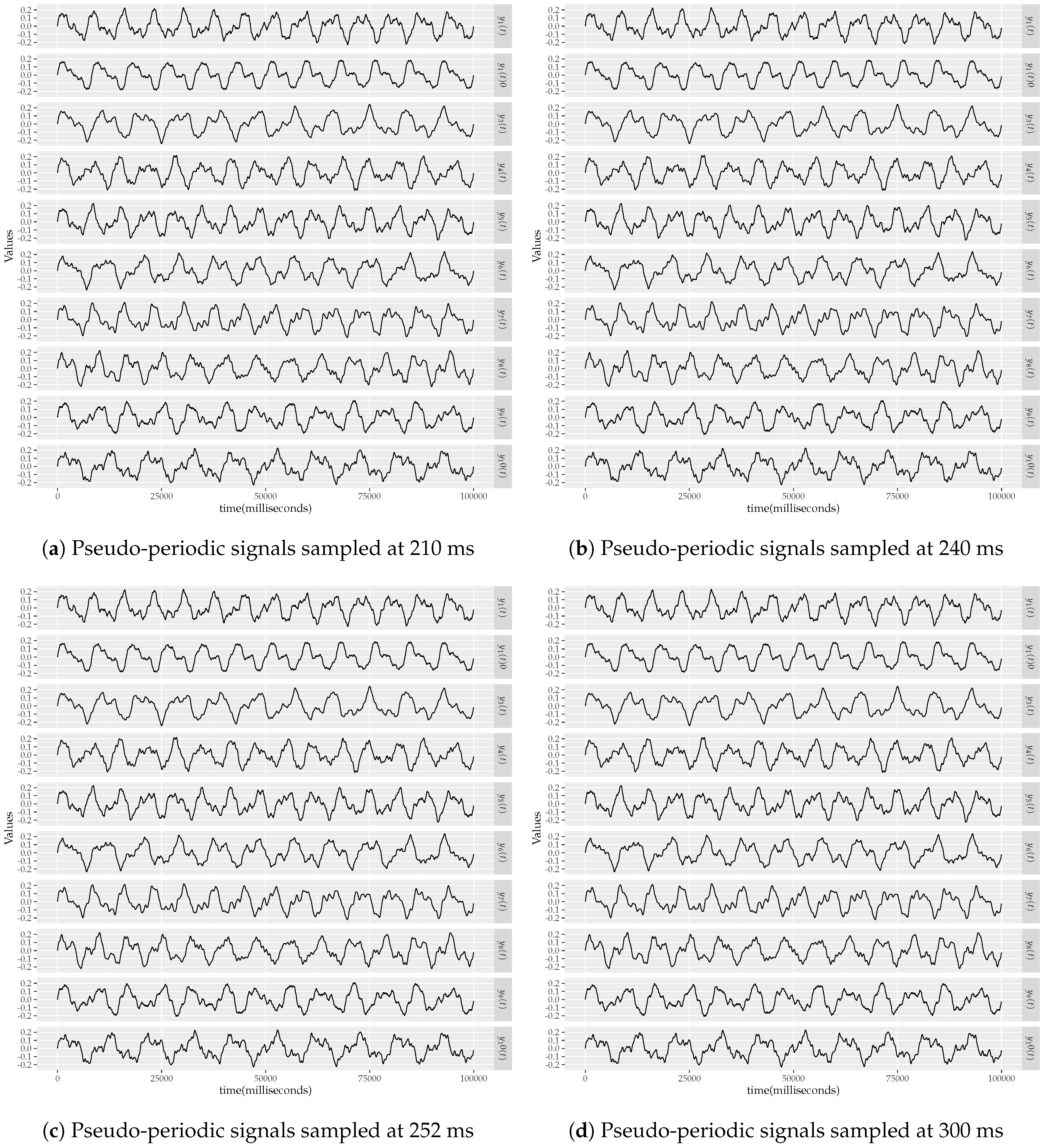
5. Simulation Results

Algorithms 1–3 were designed for runtime use when the OPC server receives samples that flow from field devices for an undefined time. In order to compare the overall performance of the algorithms, we developed an R package, named deadband, to compute each algorithm over a preloaded time series in a defined time interval.

The moving average and Bollinger band functions were imported from the package TTR developed in Reference [34]. The preloaded time series in the deadband package were generated from sampling the public dataset Pseudo Periodic Synthetic Time Series from the UC Irvine KDD Archive [35] built in Reference [36].

The original dataset, before sampling, used to generate the subset in the deadband package, was built by using Equation (11):

$$y\left(t\right)=\sum _{i=3}^7\frac{1}{2^i}sin\left(2\pi \left(2^{2+i}+rand\left(2^i\right)\right)\overrightarrow{t}\right)0\le \overrightarrow{t}\le 1.$$

(11)

The original dataset was made up of ten series of 100,000 data points generated from $t=0$ and $t=1$, and the amplitude values ranged from $-0.5$ to $+0.5$. Each of the ten series represents a pseudo-periodic signal $y\left(t\right)$. These signals can be considered a random mix of ramp, step, and pseudo=periodic sinusoidal signals such as in real manufacturing production plants using OPC gateways [37].

Since, in most OPC servers, the $ServerScanRate$ is pre-configured between 200 and 300 ms, the simulations are grouped using all sampling rates. The preloaded dataset in the deadband package was generated from the original dataset of Equation (11) by sampling all ten pseudo-periodic times series at 210 ms, 240 ms, 252 ms, and 300 ms rates [38]. Figure 2a–d show plots of all ten signals sampled at 210, 240, 252, and 300 ms respectively and ordered from $y_1\left(t\right)$ to $y_{10}\left(t\right)$.

For construction, all of the generated pseudo-periodic signals $y_i\left(t\right)$ have already defined engineering unit (EU) upper and lower bounds of:

• $E{U}_{max}=+0.5$, and
• $E{U}_{min}=-0.5$,

respectively.

The simulations explored the filtering effectiveness and the fidelity by using the Euclidian distance between the reconstructed signals at the SCADA/OPC client, after the deadband processing was computed at the OPC server. The deadband package includes the functions deadbandAD, deadbandBD, and deadbandVD to compute the AD, BD, and VD deadband algorithms. All functions process the algorithms over a limited time interval in order to generate data for comparisons.

Using the preloaded time series in the deadband package, the code in algorithm 1 shows an example of the deadbandAD code function when it processes the first time series in the first column of the preloaded data table, which is related to sampling at 240 ms. The offset parameter represents the number of samples shifted out before beginning the calculation of the moving average in the deadbandBD and deadbandVD functions. This parameter was also included in the deadbandAD function in order to align the simulation results in the same time interval. The simulation shows the use of the deadbandBD and deadbandVD algorithms with deadband percentage $d=0.01$, the period $n=20$, and the multiplier $k=2$.

In all evaluated simulations in this paper, the adopted values of the d parameter were 0.001, 0.01, 0.02, 0.05, 0.10, 0.20, 0.30, 0.45, 0.60, and 0.99. In order to consider all d values, the functions deadbandAD, deadbandBD, and deadbandVD were repeated in a simulation loop in an R script.

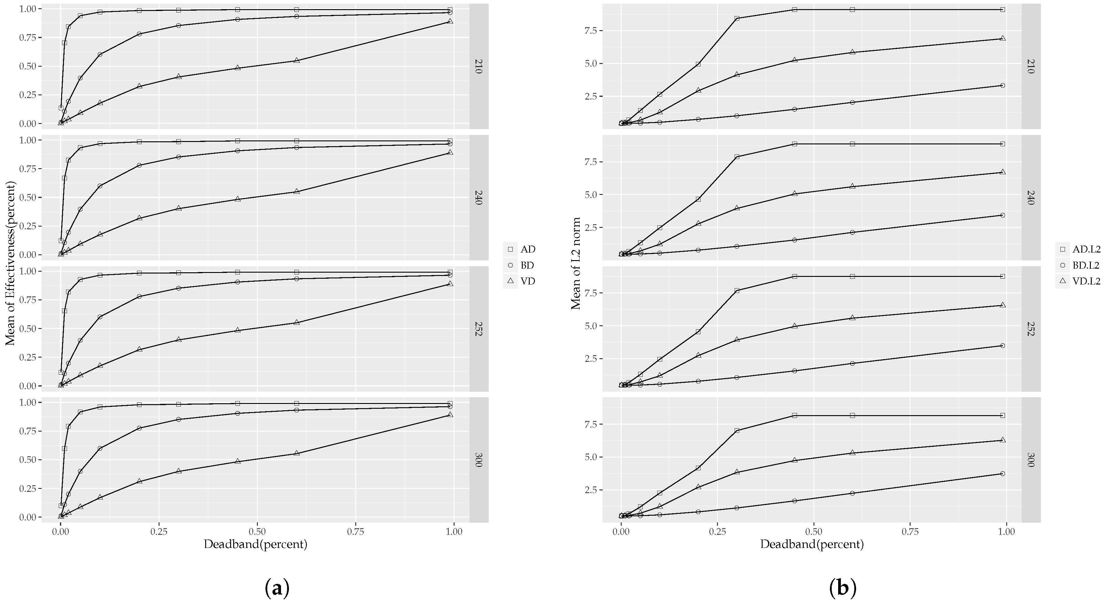
5.1. Effectiveness and Fidelity

The mean rate of messages $\lambda$ is defined as the mean number of transmissions per unit time. In the SoD scheme, the effectiveness p is defined as the reduction of the mean rate of messages in comparison to periodic sampling for a given resolution [39,40,41]. It is defined by Equation (12):

$$p=\frac{{\lambda }_T}{\lambda }$$

(12)

where ${\lambda }_T$ is frequency in the periodic sampling scheme and $\lambda$ is the mean rate of messages in the SoD scheme. Since, in our scenario, the samples reported by the OPC server are a subset of the samples received from the field sensors, we express the effectiveness as the ratio of samples reported by the deadband algorithm and the total number of samples for the evaluated sampling rate: 210 ms, 240 ms, 252 ms, and 300 ms.

The mean effectiveness for all $y_i\left(t\right)$, with $i=1,\dots ,10$, grouped by sampling rate, is shown in Figure 3a. In Figure 3a, an increase in the number of filtered samples, by tuning the d parameter, results in a smoother curve for the VD algorithm. This effect permits more granularity in tuning the d parameter using the VD algorithm than the AD algorithm.

Fidelity is a measure of the similarity between the original signal sampled at the $ServerScanRate$ and the remote reconstructed signal by using the samples reported by the deadband algorithm. The L2 norm distance was computed for all $y_i\left(t\right)$, with $i=1,\dots ,10$. The results for each sampling rate group, given as means over all $y_i\left(t\right)$, are shown in Figure 3b. In Figure 3b, the distance performed by the VD algorithm is represented by the lower curve of the L2 norm mean. This simulation of the signals reconstructed from the samples filtered by the VD algorithm presents a higher fidelity than the corresponding AD and BD algorithms for the same values of d.

Table 2. Averages of effectiveness and fidelity values calculated for each simulated sampling rate, after normalization.

	Effectiveness			Fidelity
d	AD	BD	VD	AD	BD	VD
0.01	66%	11%	2%	5%	5%	5%
0.05	92%	40%	9%	13%	5%	7%
0.1	96%	60%	17%	25%	6%	12%
0.2	97%	77%	31%	46%	8%	28%

presents the averages of the normalized effectiveness and fidelity, calculated for the sampling rates of 210, 240, 252, and 300 ms. For values of d up to 0.2, the numerical results in Table 2 show a reduction of samples when using the BD algorithm, more than twice as much as when using the VD algorithm. Additionally, in terms of the distance of the reconstructed signal from the original signal, the BD algorithm reports lower L2 norm values than the VD approach. In terms of the granularity of the effectiveness results by tuning the d parameter, the graphs in Figure 3a show a smoother evolution of the VD curves than BD for d values over 0.2.

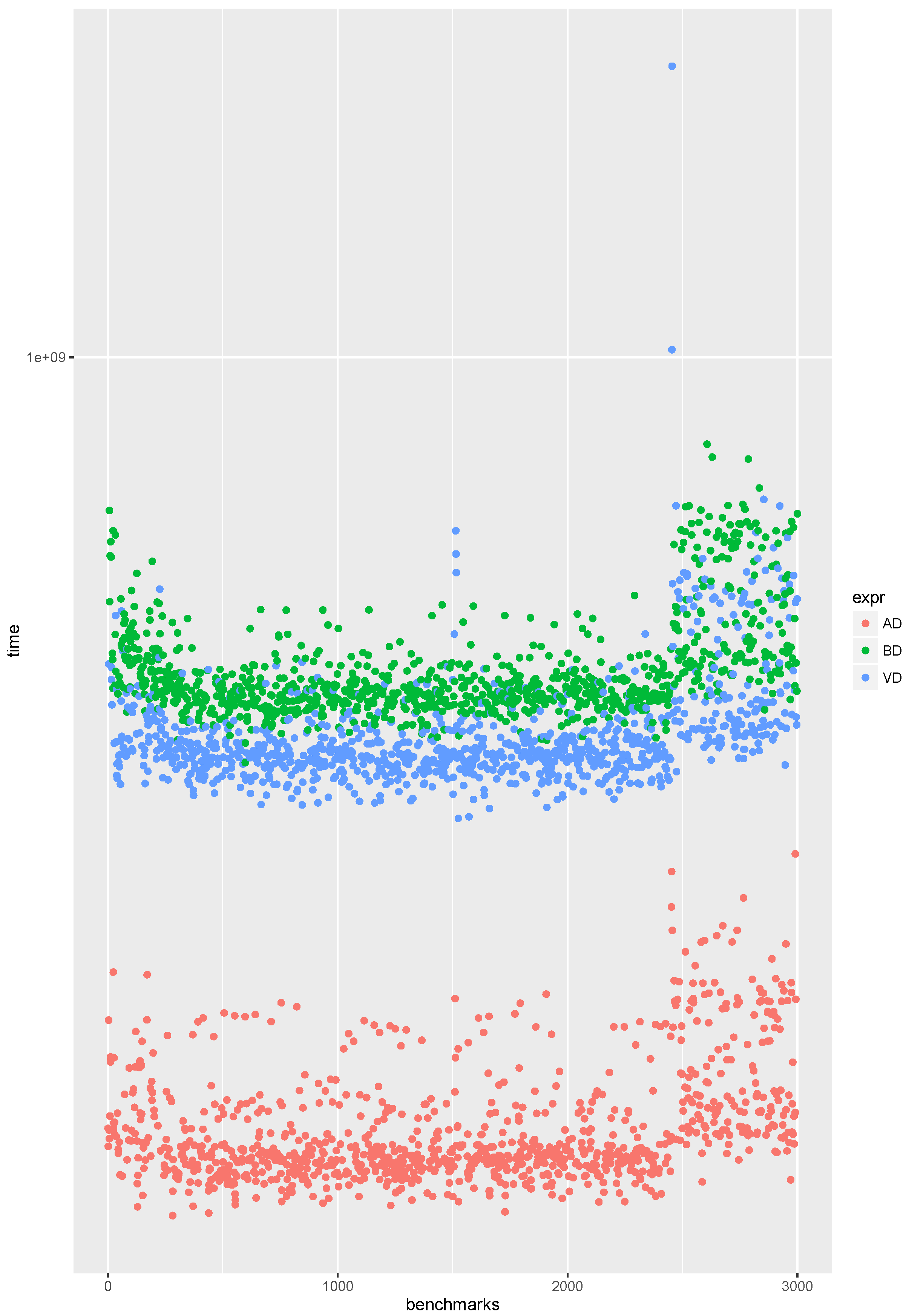
5.2. CPU Usage Benchmarks

Since the application domain of these algorithms is mainly in embedded systems, a comparison of the CPU time usage was evaluated using the microbenchmarks package [42]. Figure 4 shows the mean of the overall CPU time used to compute all $y_i\left(t\right)$, with $i=1,\dots ,10$, for each of the algorithms: AD, BD, and VD. The CPU time measurement test was repeated 1000 times for each algorithm and thus we have 3000 benchmarks on the x-axis. The log scale in y expands the visual difference between the computation time of the BD and VD approaches. These two algorithms, as expected due to the presence of the moving average, require more CPU time than the AD algorithm. The increase in the mean CPU time from the AD to the BD algorithm was about 79%, while the increase from the AD to the VD algorithm was about 66%.

6. Conclusions

This study’s approach was partially statistical, because it adopted a financial theory used on the stock market, but the evaluation of the simulation results followed the metrics of effectiveness and fidelity for signal processing. The objective was to use the statistical approach in order to design a new family of algorithms for gateways of fieldbus networks, embedded systems, and remote sensors monitored by SCADA/OPC systems. The original family of statistical SoD or deadband schemes includes two algorithms: the Bollinger deadband (BD) and volatility deadband (VD) approaches. The fidelity was measured as the L2 norm distance. An increase in the L2 norm distance means a decrease in fidelity because the reconstructed signal is more distant from the original signal. Therefore, the signals reconstructed by using the samples of BD can be considered closer to the original signal than the VD algorithm. On the other hand, the signals filtered by the VD algorithm are quantitatively sampled more than those filtered by the BD algorithm, as reported in the effectiveness shown in Figure 3a.

References

1. Friedman, M.F. Statistical Analysis of Deadband-deviation Rules in Quality Control. Comput. Oper. Res. 1995, 22, 419–433. [Google Scholar] [CrossRef]
2. Ellis, P. Extension of phase plane analysis to quantized systems. IRE Trans. Autom. Control 1959, 4, 43–54. [Google Scholar] [CrossRef]
3. Liu, Q.; Wang, Z.; He, X.; Zhou, D. A survey of event-based strategies on control and estimation. Syst. Sci. Control Eng. 2014, 2, 90–97. [Google Scholar] [CrossRef]
4. Sijs, J.; Lazar, M. On event based state estimation. In International Workshop on Hybrid Systems: Computation and Control; Springer: Berlin/Heidelberg, Germany, 2009; pp. 336–350. [Google Scholar]
5. Damm, M.; Leitner, S.H.; Mahnke, W. OPC Unified Architecture; Springer: Berlin/Heidelberg, Germany, 2009. [Google Scholar]
6. Bitter, R.; Mohiuddin, T.; Nawrocki, M. LabView: Advanced Programming Techniques, 2nd ed.; CRC Press: Boca Raton, FL, USA, 2006. [Google Scholar]
7. Loy, D.; Dietrich, D.; Schweinzer, H.J. Open Control Networks: LonWorks/EIA 709 Technology; Springer: Berlin/Heidelberg, Germany, 2001. [Google Scholar]
8. Miskowicz, M. Event-Based Control and Signal Processing; CRC Press: Boca Raton, FL, USA, 2015. [Google Scholar]
9. Plonnigs, J.; Neugebauer, M.; Kabitzsch, K. A traffic model for networked devices in the building automation. In Proceedings of the 2004 IEEE International Workshop on Factory Communication Systems, Vienna, Austria, 22–24 September 2004. [Google Scholar]
10. R Core Team. R: A Language and Environment for Statistical Computing; R Foundation for Statistical Computing: Vienna, Austria, 2016. [Google Scholar]
11. Torrisi, N. Deadband: Statistical Deadband Algorithms Comparison. 2016. Available online: https://CRAN.R-project.org/package=deadband (accessed on 5 December 2018).
12. Diaz-Cacho, M.; Delgado, E.; Barreiro, A.; Falcón, P. Basic send-on-delta sampling for signal tracking-error reduction. Sensors 2017, 17, 312. [Google Scholar] [CrossRef] [PubMed]
13. Díaz-Cacho, M.; Delgado, E.; Prieto, J.A.; López, J. Network adaptive deadband: Ncs data flow control for shared networks. Sensors 2012, 12, 16591–16613. [Google Scholar] [CrossRef] [PubMed]
14. Hirche, S.; Hinterseer, P.; Steinbach, E.; Buss, M. Network traffic reduction in haptic telepresence systems by deadband control. In Proceedings of the 2005 IFAC World Congress, Prague, Czech Republic, 3–8 July 2005. [Google Scholar]
15. Suh, Y.S. Send-on-delta sensor data transmission with a linear predictor. Sensors 2007, 7, 537–547. [Google Scholar] [CrossRef]
16. Vasyutynskyy, V.; Kabitzsch, K. Deadband Sampling in PID Control. In Proceedings of the 2007 5th IEEE International Conference on Industrial Informatics, Vienna, Austria, 23–27 June 2007. [Google Scholar]
17. Torrisi, N.M. Monitoring Services for Industrial. IEEE Ind. Electron. Mag. 2011, 5, 49–60. [Google Scholar] [CrossRef]
18. Seilonen, I.; Tuovinen, T.; Elovaara, J.; Tuomi, I.; Oksanen, T. Aggregating OPC UA servers for monitoring manufacturing systems and mobile work machines. In Proceedings of the 2016 IEEE 21st International Conference on Emerging Technologies and Factory Automation (ETFA), Berlin, Germany, 6–9 September 2016; pp. 1–4. [Google Scholar]
19. Garcia, E.; Antsaklis, P.J. Model-based event-triggered control with time-varying network delays. In Proceedings of the 2011 50th IEEE Conference on Decision and Control and European Control Conference, Orlando, FL, USA, 12–15 December 2011; pp. 1650–1655. [Google Scholar]
20. Miskowicz, M. Send-on-delta Concept: An Event-based Data Reporting Strategy. Sensors 2006, 6, 49–63. [Google Scholar] [CrossRef]
21. Lehmann, D.; Lunze, J. Extension and experimental evaluation of an event-based state-feedback approach. Control Eng. Pract. 2011, 19, 101–112. [Google Scholar] [CrossRef]
22. Yook, J.K.; Tilbury, D.M.; Soparkar, N.R. Trading computation for bandwidth: Reducing communication in distributed control systems using state estimators. IEEE Trans. Control Syst. Technol. 2002, 10, 503–518. [Google Scholar] [CrossRef]
23. Otanez, P.; Moyne, J.R.; Tilbury, D. Using Deadbands to Reduce Communication in Networked Control Systems. In Proceedings of the 2002 American Control Conference, Anchorage, AK, USA, 8–10 May 2002; pp. 3015–3020. [Google Scholar]
24. Pantoni, R.P.; Torrisi, N.; Brandao, D. An Open and Non-proprietary Device Description for Fieldbus Devices for Public IP Networks. In Proceedings of the 2007 5th IEEE International Conference on Industrial Informatics, Vienna, Austria, 23–27 June 2007; pp. 189–194. [Google Scholar]
25. Simon, R.; Diedrich, C.; Riedl, M.; Thron, M. Field Device Integration. In Proceedings of the ETFA 2001—8th International Conference on Emerging Technologies and Factory Automation, Antibes-Juan les Pins, France, 15–18 Octorber 2001; pp. 150–155. [Google Scholar]
26. Nguyen, V.H.; Suh, Y.S. Improving estimation performance in networked control systems applying the send-on-delta transmission method. Sensors 2007, 7, 2128–2138. [Google Scholar] [CrossRef] [PubMed]
27. Åström, K.J.; Bernhardsson, B. Comparison of Riemann and Lebesque sampling for first order stochastic systems. In Proceedings of the 41st IEEE Conference on Decision and Control, Las Vegas, NV, USA, 10–13 December 2002; pp. 2011–2016. [Google Scholar]
28. Li, S.; Sauter, D.; Xu, B. Fault isolation filter for networked control system with event-triggered sampling scheme. Sensors 2011, 11, 557–572. [Google Scholar] [CrossRef] [PubMed]
29. Bollinger, J. Bollinger on Bollinger Bands; McGraw-Hill Education: New York, NY, USA, 2001. [Google Scholar]
30. Ngan, H.Y.; Pang, G.K. Novel Method for Patterned Fabric Inspection Using Bollinger Bands. Opt. Eng. 2006, 45, 87202. [Google Scholar]
31. Chande, T.S. Adapting Moving Averages to Market Volatility. Stock Commodities 1992, 10, 3. [Google Scholar]
32. Butler, M.; Kazakov, D. A learning adaptive Bollinger band system. In Proceedings of the 2012 IEEE Conference on Computational Intelligence for Financial Engineering Economics (CIFEr), New York, NY, USA, 29–30 March 2012; pp. 1–8. [Google Scholar]
33. Leeds, M. Bollinger Bands Thirty Years Later. arXiv, 2012; arXiv:1212.4890. [Google Scholar]
34. Ulrich, J. TTR: Technical Trading Rules. 2016. Available online: https://CRAN.R-project.org/package=TTR (accessed on 5 December 2018).
35. Intel. Berkeley Research lab, Sensors Data. 2004. Available online: http://db.csail.mit.edu/labdata/labdata.html (accessed on 5 December 2018).
36. Park, S.; Lee, D.; Chu, W.W. Fast Retrieval of Similar Subsequences in Long Sequence Databases. In Proceedings of the 1999 Workshop on Knowledge and Data Engineering Exchange (KDEX’99), Chicago, IL, USA, 7 November 1999; pp. 60–67. [Google Scholar]
37. Santos, R.A.; Normey-Rico, J.E.; Gómez, A.M.; Arconada, L.F.A.; de Prada Moraga, C. OPC based distributed real time simulation of complex continuous processes. Simul. Model. Pract. Theory 2005, 13, 525–549. [Google Scholar] [CrossRef]
38. Yuvaraj, D.; Ranjith, S.M.; Kumar, J.N.; Krishnan, R.H. Design and Simulation of Thermal Power Plant Using PLC and SCADA. Program. Device Circuits Syst. 2016, 8, 228–232. [Google Scholar]
39. Miskowicz, M. Analytical approximation of the uniform magnitude-driven sampling effectiveness. In Proceedings of the 2004 IEEE International Symposium on Industrial Electronics, Ajaccio, France, 4–7 May 2004; pp. 407–410. [Google Scholar]
40. Miskowicz, M. Efficiency of Event-Based Sampling according to Error Energy Criterion. Sensors 2010, 10, 2242–2261. [Google Scholar] [CrossRef] [PubMed]
41. Staszek, K.; Koryciak, S.; Miskowicz, M. Performance of Send-on-delta Sampling Schemes with Prediction. In Proceedings of the 2011 IEEE International Symposium on Industrial Electronics, Gdansk, Poland, 27–30 June 2011. [Google Scholar]
42. Mersmann, O. Microbenchmark: Accurate Timing Functions. 2015. Available online: https://CRAN.R-project.org/package=microbenchmark (accessed on 5 December 2018).
Figure 1. Overview of the steps to receive the samples at the OPC client.
Informatics 06 00005 g001
Figure 2. Pseudo-periodic signals sampled at (a) 210, (b) 240, (c) 252, (d) 300 milliseconds.
Informatics 06 00005 g002
Figure 3. Effectiveness and L2 norm comparison for AD, VD and BD algorithms. (a) Mean of deadband effectiveness over all signals grouped by sampling rate; and (b) Mean of L2 norm over all deadband signals grouped by sampling rate.
Informatics 06 00005 g003
Figure 4. Computation benchmark comparison.
Informatics 06 00005 g004