Article

A Review and Characterization of Progressive Visual Analytics

by
Marco Angelini
1,
Giuseppe Santucci
1,
Heidrun Schumann
2 and
Hans-Jörg Schulz
3,*,†
1
Sapienza University of Rome, 00185 Rome, Italy
2
University of Rostock, 18059 Rostock, Germany
3
Aarhus University, 8000 Aarhus Aarhus, Denmark
*
Author to whom correspondence should be addressed.
Current address: Åbogade 34, 8200 Aarhus N, Denmark.
Informatics 2018, 5(3), 31; https://doi.org/10.3390/informatics5030031
Submission received: 16 May 2018 / Revised: 27 June 2018 / Accepted: 30 June 2018 / Published: 3 July 2018

Abstract

:
Progressive Visual Analytics (PVA) has gained increasing attention over the past years. It brings the user into the loop during otherwise long-running and non-transparent computations by producing intermediate partial results. These partial results can be shown to the user for early and continuous interaction with the emerging end result even while it is still being computed. Yet as clear-cut as this fundamental idea seems, the existing body of literature puts forth various interpretations and instantiations that have created a research domain of competing terms, various definitions, as well as long lists of practical requirements and design guidelines spread across different scientific communities. This makes it more and more difficult to get a succinct understanding of PVA’s principal concepts, let alone an overview of this increasingly diverging field. The review and discussion of PVA presented in this paper address these issues and provide (1) a literature collection on this topic, (2) a conceptual characterization of PVA, as well as (3) a consolidated set of practical recommendations for implementing and using PVA-based visual analytics solutions.

Graphical Abstract

1. Motivation

With data growing in size and complexity, and analysis methods getting more sophisticated and computationally intensive, the idea of Progressive Visual Analytics (PVA) [1,2] becomes increasingly appealing. A PVA approach can either subdivide the data to process each data chunk individually, or it can subdivide the analytic process into computational steps that iteratively refine analytic results [3]. By doing so, PVA yields partial results of increasing completeness or approximative results of increasing correctness, respectively. This is useful in a wide range of visual analytics scenarios:
  • to realize responsive client-server visualizations using incremental data transmissions [4],
  • to make computational processes more transparent through execution feedback and control [5],
  • to steer visual presentations by prioritizing the display of regions of interest [6],
  • to provide fluid interaction by respecting human time constraints [7], or
  • to base early decisions on partial results, trading precision for speed [8].
Because of its versatility, the progressive approach to data analysis and visualization is alternatively seen as a paradigm for computation, for interaction, for data transmission, or for visual presentation. It is thus not surprising that PVA-related research is distributed over multiple disciplines, motivated by various underlying problems, described in different, sometimes overloaded terms at different levels of detail for different audiences.
In this paper, we aim to give a comprehensive answer to the question What is Progressive Visual Analytics? We do so by putting forth a multi-faceted characterization that reflects the main perspectives on the subject, as they are described in the fragmented body of scientific literature on this topic. Concretely, this paper makes three contributions:
  • a collection and review of scholarly publications on the topic of PVA from various domains;
  • a characterization of PVA capturing the reasons, benefits, and challenges of employing it;
  • a set of recommendations for implementing PVA sourced from a range of publications.
As the field of PVA is still emerging, the presented collection of publications as well as the characterization and recommendations derived from them should not be mistaken for a survey that aims to wrap-up a mature field of research. Instead, they should rather be understood as an overview of the current understanding of PVA that bundles the research results achieved so far and serves as a stepping stone for new ones. In order to make this overview practically useful, we adopt an output-oriented, utility-driven perspective on PVA that looks at the existing literature from an angle that asks What can it do for me? and How can I make it do that? Due to this output-oriented perspective, this overview leans somewhat to the visualization and interaction side and focuses on discussing the existing approaches from that end user perspective. In that sense, this paper complements existing works focusing more on the computational angle [2,3,5].
The paper is structured as follows: After giving a brief introduction into PVA in Section 2, we outline our procedure by which we have conducted this literature review in Section 3. We then detail our characterization of PVA in Section 4, before discussing practical requirements for realizing PVA and distilling them into recommendations in Section 5. Finally, we describe a use case example from our own work to illustrate how we applied some of those recommendations in a real-world PVA scenario in Section 6. Section 7 concludes this paper and gives an outlook on promising directions for future work in this area.

2. PVA Fundamentals

Progressive Visual Analytics (PVA) “produces partial results during execution” [1]. This central concept is also known as Fine-Grain Visualization [9], Online Visualization [10], Incremental Visualization [8], Progressive Visualization [11], Per-Iteration Visualization [12], Optimistic Visualization [13], Approximate Visualization [14], and Progressive Analytics [2]. As a common denominator, these all generate intermediary visualization outputs while the data is still being processed.
PVA is often discussed in relation to two other forms of visual analytics: Monolithic Visual Analytics (MVA) and Instantaneous Visual Analytics (IVA) [15]. MVA is the typical way of going about data analysis by processing the whole dataset in one big algorithmic procedure without yielding intermediate results. While in this context the term monolithic may be overloaded, no other, more fitting and better delineated term has emerged yet for MVA-type analysis procedures. Whereas IVA usually employs some form of preprocessing in order to make analysis results for the whole dataset available without delay. Such preprocessed results—either data [16] or prerendered views [17]—are stored in databases, so that they need only to be retrieved, but not computed any more. This way, the analyst can interactively explore different parameter settings and get instantaneous feedback, as the results for each parameter combination can be swiftly queried from that database. All three visual analytics paradigms are schematically depicted in Figure 1.
PVA can be a complex approach with many intricacies and details to be considered. As a starting point for discussing PVA, its behavior can be summarized as follows: After starting out, it produces a first meaningful partial result at time point t Response . “Meaningfulness” means that it must be indicative of the final result, effectively ruling out progress bar displays and mere placeholders like empty coordinate axes. From this time point onward, PVA produces early partial results with which the user can already interact as if interacting with the final result—just not yet with the still missing data points or visual details. PVA then proceeds until at time point t Reliable the result is still approximate, but already reflects the final result within an acceptable margin of error. From this time point onward, PVA produces mature partial results that are trustworthy enough to start exploring the data and to make first observations and findings. As the PVA process continues to run, it will produce the last significant update at time point t Stable after which the remaining updates will no longer change the overall result in any substantial way. From this time point onward, PVA produces definitive partial results that are close enough to the final result to be used in its place—for example, to verify the still uncertain findings from before. If the findings hold up, they become confirmed insights into the data [18]. And all this happens, before the final result is produced at time point t Complete .
Note that t Complete of PVA may actually exceed t Complete of MVA. This is usually due to the computational overhead of producing and managing the incremental updates. Yet this drawback is only a theoretical one, for two reasons:
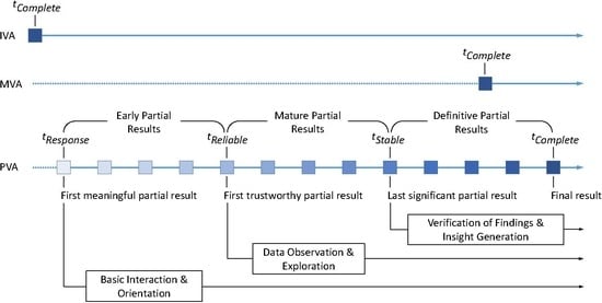
  • With PVA, we are able to start the interactive analysis right after t Response in parallel to the further refinement of the view. Yet with MVA, view generation and interactive analysis can only be done in sequence, so that the overall time spent on generating and utilizing the visualization extends well beyond t Complete .
  • With PVA, we yield a sufficiently good partial result as early as t Reliable and no later than t Stable , which is in most cases still well before MVA’s completion time. PVA’s t Complete is irrelevant, since if we wanted a final and polished result, we would have used MVA in the first place.
PVA can generate results in two ways: by subdividing the data and processing it chunk by chunk, or by subdividing the computational process and executing it step by step. In the first case, which we call data chunking, the partial results show increasingly more data over time, until at t Complete all the data is shown in the final output. Whereas in the second case, which we call process chunking, the partial results show all the data all the time, but the quality of the rendering increases with each step—from a quick and dirty first view at t Response to an elaborately refined final view at t Complete . In principle, it is also possible to combine both strategies [3]. But this is rarely done. One reason observed in recent user studies may be that users seem uneasy to judge the trustworthiness of partial data shown in unfinished visualizations at the same time [19].
The description of PVA put forth in this section follows the output-driven perspective mentioned in the introduction by using discrete time points to partition the progression into stages of different analytical utility. This characterization mirrors recent research in activity-centered visualization design that assesses a visualization based on the tasks and activities it supports [20], instead of just looking at how faithful it represents the data (cp. representational primacy [21]). Yet, the resulting staged model of PVA neither invalidates, nor supersedes the understanding of PVA as a continuous stream of results that improves over time, as formulated for example by Fekete and Primet [2] and as signified by the blue squares in Figure 1—but rather complements it. This is in particular so, as the stages assumed by the model are hardly fixed, easy to determine, or even well-defined, because they are highly dependent on the data, the task, the user, and the domain. But for the remainder of the paper, the four time points and the intervals in between them provide us with an abstraction of a PVA run that serves as a relatable and meaningful frame of reference to which we can map the highly heterogeneous body of literature on one hand, and to which the readers can map their own PVA scenario or use case on the other hand.

3. Review Procedure

According to Fink [22] (p. 3), “a research literature review is a systematic, explicit, and reproducible method for identifying, evaluating, and synthesizing the existing body of completed and recorded work produced by researchers, scholars, and practitioners”. This section is about the first part of this definition—i.e., where we make explicit our method for conducting this review, so that its systematic nature is documented and can be reproduced by others. Our literature review on the topic of PVA entailed six steps:
(Step 1) Gathering literature on PVA. To collect PVA-related publications, we used the common approach of a set of initial seed publications on the topic of PVA from various disciplines. Using Google Scholar, we retrieved the set of all papers they cite, as well as all papers citing them. For all PVA-related papers among them, we repeated this process, until no further PVA-related papers were found. The set of initial publications included 15 papers from various disciplines: Databases [23,24,25,26,27], Information Visualization [3,28], Scientific Visualization [9,11], Visual Analytics [1,2,5,7], and Human–Computer Interaction (HCI) [4,8]. The results of this step are listed in the Reference Section at the end of this paper.
(Step 2) Extracting different PVA concepts. We then went over all gathered papers with the aim of extracting the different notions of PVA they describe. For the largest part, these notions align with the scientific community in which the respective papers are published. For example, PVA papers from the HCI community tend to focus on PVA as a means to facilitate interaction, whereas papers from the Database community tend to position PVA as a means to produce database query results. It soon became clear, that most papers put their own little twist on the basic idea of progression, which results in a quite diverse and nuanced understanding of PVA with each PVA system or algorithm instantiating their own PVA concept. Hence, the result of this step was the realization that the understanding of PVA is much too heterogeneous to discuss it bottom up by merely collecting all its different notions.
(Step 3) Consolidating concepts in a characterization of PVA. To nevertheless get a grasp on the body of literature, we thus proceeded to no longer look for distinctions between the various notions, but for their commonalities, disregarding different terminologies and levels of detail. We found that most instances of PVA note some reasons why it is employed in the first place and some PVA benefits that are exploited to address the reasons. Moreover, papers often discuss additional challenges of using PVA. Breaking up PVA along these three aspects captures that there are different reasons for using PVA, which are addressed by different PVA benefits and lead to different PVA challenges. The characterization according to PVA’s reasons, benefits, and challenges is given in Section 4.
(Step 4) Extracting practical requirements for PVA. The existing body of literature offers various ways in which to provide the PVA benefits and to resolve, circumvent, or at least reduce the PVA challenges. To that end, a number of publications give practical advice on which additional features to provide and what design criteria to observe to realize an effective and usable instance of PVA. We collected this advice as requirements from these papers and we present this “raw” collection in Appendix A1.
(Step 5) Aligning requirements with PVA characterization. Having the collection of requirements is just one side of the coin. We still need to know when to follow which one. For this reason, we drew connections between the various requirements by grouping them in a process-driven way, and in a user-driven way. The results of this step are detailed in Section 5. The process-driven grouping is done with respect to the aspect of the visual analytics process to which they pertain. And the user-driven grouping is done with respect to the PVA characterization given in Section 4, i.e., the PVA benefits they aim to provide and the PVA challenges they aim to address. As a result of this step, we distill nine high-level recommendations from the various requirements—one for each identified benefit and challenge.
(Step 6) Exemplification of PVA characterization and recommendations. Finally in this last step, we aim to put our PVA characterization and the proposed recommendations in the context of a real world use case. For this step, we have chosen one of our own PVA solutions for the simple reason that we have all the necessary inside information on why and how we built it, so that we can discuss it in the necessary depth. This discussion is given in Section 6.

4. A Characterization of PVA

PVA is no end in itself. Instead, PVA is used in response to various shortcomings posed by MVA in certain analysis scenarios. We call these shortcomings the reasons for using PVA. Producing intermediate results translates into a number of benefits that counter these shortcomings when using PVA instead of MVA. Yet PVA also incurs additional challenges for the developer and the user to deal with. In the following, we detail the different reasons, benefits, and challenges of PVA.

4.1. Reasons for Using PVA

Going through the literature, we can find three main reasons why PVA is used instead of MVA. These reasons all relate to the computational process—i.e., the dotted line shown for MVA in Figure 1 indicating the wait time for the result: it lasts too long (duration), it runs too slow (speed), and it is non-transparent in its course.
Long-lasting computations. In this case, the main problem is the completion time t Complete of the computation being well beyond the acceptable. Possible instances are:
  • Indefinite computations: These are computations having no defined end by design, such as visualizations for monitoring transient data streams [29,30,31].
  • Quasi-indefinite computations: These are computations that will theoretically terminate at some point, but reaching this point is a few thousand years out, e.g., due to combinatorial explosion [32].
  • Delayed computations: These types of computations can be completed within reasonable time, but it is still taking too long to meet a given deadline by which the result is needed.
This list purposefully abstracts from the various technical causes that such unacceptable runtimes can have. This can be either an inherent complexity of the problem—the data may be very complex (e.g., having hundreds of dimensions or being very heterogeneous) or the algorithms to be run on it may exhibit a high complexity that simply take time to complete. Or it can be that insufficient resources are available—e.g., the memory may be too small for the data so that swapping takes up a large portion of the time, or the network connection over which the data is loaded may be slow. While there can be a multitude of these underlying causes, which sometimes may even compound each other, the result will always be one of the three instances listed above.
Slow computations. Here, the shortcoming is that the completion time t Complete is not within bounds for fluid interaction [33] including guaranteed response times to queries and continuous manipulation of views. Expected response times are commonly subdivided in three levels [2,34,35]:
  • Task completion: Initiating a computational task, such as a query or complex filter operation on large datasets, should not stall the flow of analysis for more than 10 s.
  • Immediate response: In an interactive setting, such as tuning computational parameters in a GUI, feedback to the made changes should appear in 1 s.
  • Perceptual update: Computations initiated through direct interaction with the view should complete in under 1 s to ensure smooth updates without noticeable stutter or flickering.
Note that long-lasting and slow computations, and in particular delayed and slow computations, are discerned by their effects and not so much by their causes. Long-lasting computations make it impossible to use their results—for visual analysis or otherwise—as the delay does not permit to act upon the result in time. An example would be to forecast tomorrow’s weather or stock prices by the day after tomorrow. Whereas slow computations pose no principal hindrance to using their results. It may just become more tedious and less effective, as it has been shown that already minor latencies have negative impacts on insight generation [36].
Non-transparent computations. Papers arguing from this perspective criticize the monolithic, one-step nature of the computation that gives MVA its name. They note that MVA presents an algorithmic black box without any means to observe, interject, and reconfigure it on the fly. Its only means of understanding the computation is after the fact by inferring what might have happened from the result produced at completion time t Complete . This argument is delivered from two different angles:
  • Monolithic computations: In this instance, the focus lies on the complexity and opacity of the computational process that cannot be observed, understood, or steered while running its course [5].
  • Monolithic visualizations: Here the focus lies on the visualization produced by the process and being shown in all its cluttered, overplotted detail as a single monolithic end result [6].
Note that non-transparency is an independent reason from the computations’ runtime. In fact, a computation can actually be completed in a matter of seconds and its non-transparency is the result of its speed, as it is too fast to monitor or adjust the execution while it is running. So, it could even be necessary to introduce intentional deceleration to decrease its speed and increase its duration to enable observation and steering of the process in the first place.
These three reasons—duration, speed, and transparency—are often not clearly separated from each other. This is not surprising as in MVA, all problems and shortcomings relate to the one and only result produced at time point t Complete , which is the first meaningful, the first reliable, the last significant, and the final result all in one. PVA, however, allows for a more nuanced discussion of these aspects.

4.2. Benefits of Using PVA

The defining and distinguishing factor of PVA is its ability to produce a sequence of results. This sequence is largely defined by the four characteristic time points introduced in Section 2: t Response at which the first meaningful partial result is produced, t Reliable at which the first trustworthy partial result is produced, t Stable at which the last significant partial result is produced, and t Complete at which the computation finishes. These create three time intervals in which results of different quality and utility are produced:
Early partial results. These are produced between t Response and t Reliable . Therefore, they are meaningful, but not necessarily reliable yet. An example for such an early partial result would be a preview that gives already a first visual indication of the overall look and feel of the final visualization, but without yet showing enough data to draw conclusions from it. Showing such a preview can be used to orient oneself in the view before it gets too cluttered. If the preview is generated quickly enough—i.e., t Response stays below an acceptable update rate—it can provide fluid interaction.
Early partial results can further be used by the analyst to determine if the overall visual representation suits the analytical needs, performing an early cancellation if not. An early cancellation means that the preview is so far off from an acceptable visual result that it warrants to abort the currently running computation and to try something else. Mühlbacher et al. [5] argue that early cancellation also provides an important, albeit simple form of process control. It may not allow full-fledged computational steering, but early cancellation can be used to test different algorithms and parametrizations through trial and error.
Mature partial results. These are produced between t Reliable and t Stable . They already reflect the final result within an acceptable margin of error. Hence, they can be used for an early start of the visual analysis, as they show enough data and detail to make first observations in the still unfinished, yet already trustworthy intermediate result. In that sense, mature partial results can be used to gain a head start in time-critical analysis scenarios even before the results fully stabilize. The decision when a partial result is reliable enough to do so is:
  • process-specific: a monotonously converging progressive computation is likely to yield useful results earlier than one that is highly fluctuating and bound to produce “surprises”;
  • task-specific: a high-level overview task requires less detail to be shown than an in-depth comparison;
  • domain-specific: a social media analysis can accept a higher margin of error than analyzing patient records to make a clinical treatment decision;
  • user-specific: some users with experience in progressive computations may be able to see early on “where this is going”, while others wait a little longer before feeling comfortable to work with a partial result.
Definitive partial results. These are produced between t Stable and t Complete . In this case, the computation is not entirely finished yet and we are still dealing with partial results. These results may not yet look as polished as the final result with last minor layout optimizations still needing to be computed, or they may still miss some data points as a few remaining data chunks have not yet been processed. Yet, these results leave no more doubt about the final outcome. That final outcome can be assumed as settled at this stage and the partial results can be used in its place for all practical purposes. Hence, they can be used for an early completion of the visual analysis, confirming observations made on mature partial results and basing early analytic decisions on them. There exist two scenarios of such early completions, which we term:
  • hard early completion: this terminates the running computation and starts with the next analytical step based on the findings made up to that point;
  • soft early completion: this also starts with the next analytical step, but the computation is only paused and not terminated [1].
While the hard early completion frees processing resources for the next analysis step, the soft early completion frees CPU resources, but keeps memory resources allocated. In this way, the computation can be immediately resumed at a later point in time—e.g., after returning from an analytical detour on some matter that caught the analyst’s eye.
In principle, a third option would also be possible that neither terminates nor pauses the computation, but continues it as a background process. While this does not free any resources except for screen space, it is the safest option if unsure about the stability of the current result. In the event that the background process produces a new result exhibiting major differences, the users can be alerted. They can then inspect these differences and decide whether to roll back any follow-up analysis steps carried out since. To the best of our knowledge, this approach has so far not been documented in the literature.
From the individual partial results that PVA generates, emerges a fourth benefit of PVA:
Succession of results. Besides providing new start and end points for visual analysis, PVA also provides a constant outflow of results that lie in between. These form a string of natural “break points” that can be used to
  • monitor the computation in its course for understanding and possibly debugging the algorithmics behind it (cp. software visualization);
  • steer the computation through interactive reparametrization of algorithms or reprioritization of data chunks, adapting the PVA process to early observations and emerging analysis interests;
  • observe the build-up of complex visualizations step by step, showing increasing numbers of visual elements to convey even dense, detailed, and cluttered visualizations;
  • adapt an output to just the right level of detail so that the succession produces outputs of increasing detail [6] or decreasing detail [37], which can be stopped at any in-between stage to fit the current display space and desired visual complexity.
All of these benefits are often subsumed under the observation that PVA makes interactive visual analysis more responsive [4] and more accessible [5]. Although, it is important to note that while these benefits are inherent in the way PVA operates, they may not automatically show as desired. For example, just by employing PVA, it is not guaranteed that certain response times and update intervals are met as needed. For example, an algorithm may in principle be suited to work on continuously updating data, but each update may take so long that it is not suited for interactive visual analysis [38]. This requires careful configuration of the underlying mechanisms for chunking the data and the process, which brings us to the challenges of using PVA.

4.3. Challenges of Using PVA

The additional possibilities that PVA opens up come with the price of additional efforts: It is up to the analyst to decide how to initialize the progression and whether it runs as expected, as well as to assess the usefulness and trustworthiness of partial results. Guidelines and metrics can inform the analyst’s decisions, but in the end it remains the responsibility of the human in the loop to make these decisions. We have identified five challenges that analysts face when using PVA:
Parametrizing the progression. Running a PVA solution asks for additional efforts at both design phase and utilization phase for a suitable (for the task to be carried out) parametrization of the progressive pipeline. Common parameters for data chunking concern the sampling technique, the sample size, the processing order or prioritization of sampled data chunks, and how to combine them back together through buffering, binning, or aggregation. Common parameters for process chunking concern the step size for the iterations, the stopping criterion for when to end the progression, and sometimes also a random displacement that governs the degree of intentionally introduced fluctuation to avoid convergence towards local optima. Managing this additional parameter space, not present in MVA, clearly demands additional efforts [39]. But PVA also helps in doing so, by allowing interactive readjustment and fine-tuning of parameters while the progression is already on its way.
Judging partial results. Partial results, while being displayed promptly, come at the cost of being only approximate. They are either incomplete in case of data chunking as not all data has yet been processed, or they are inaccurate in case of process chunking as not all iterations have yet been computed. When dealing with intermediate results, the analyst has the additional burden of judging whether they are “good enough” for the analytic task at hand—i.e., whether t Reliable has been reached. This challenge does not occur in MVA, as it is clearly rooted in the progression. There are different strategies for judging partial results, such as looking at absolute completion rates (How much of the full dataset is shown? How many out of all iterations have been computed?) or looking at relative completion rates (How much additional information did a new result add to a previous one?) Note that this particular challenge gains additional complexity when multiple views are involved that exhibit different states of maturity. In this case, it is not clear on which view the user should rely to judge the current result’s trustworthiness.
Monitoring the succession of results. The partial results alone do not tell the full story. Only in the context of the series of results, we are able to judge the current one. Is the computation converging towards a stable result or is there no such trend? If it is converging, can we estimate how long until t Stable is reached? And when the output is no longer changing, have we actually reached t Stable ? Or is it just because the progression is “jammed”, dealing with the latest interactive changes we made or processing an unexpectedly complex data chunk? So, while keeping an eye on the running computation can be seen as an additional burden, it also provides additional information on the provenance of the currently shown result as an intermediate point of that computation. This can be used to further inform the reliability assessment of the current partial result, but also as an indication for the need to adjust or steer the progression.
Steering the progression. Like MVA, PVA can be run in a fire and forget manner: once set up and parametrized, it is never changed and runs its predefined course. Yet this would mean to disregard most of PVA’s inherent flexibility and thus to reduce its use to only a fraction of what it could be: a responsive mechanism with which we can interact while it is running and which can be adapted alongside our growing understanding of the data and our evolving analytic interests. Leveraging this full potential of PVA also means that the analyst cannot sit back and wait for the final result to arrive, but has to actively intervene and steer the computation. At the minimum, the analyst has control over starting, pausing, slowing down and speeding up, as well as stopping (early cancellation, early completion) the process. This can also encompass branching of an analysis into two concurrently run processes—e.g., running the same algorithm on different data, or different algorithms on the same data to compare or interleave their results. More involved forms of steering include narrowing down and refocusing the process on certain subspaces of interest within the dataset, or to halt the processing of data subspaces irrelevant to the current task or analytic question.
Handling fluctuating or even diverging progressions. Many PVA approaches assume a “well-behaved”, monotonously converging progression of results that proceeds smoothly from a crude first response to a refined final result. In practice, this is hardly ever the case: data may be non-uniformly distributed across the chunks, the computation may perform random moves to escape local optima, or the user may interact with the computation, readjusting it and thus introducing discontinuities in the process. Governing concepts like data consistency (intermediate visualizations should become increasingly representative of the complete dataset) and visual consistency (intermediate visualizations should become increasingly representative of the completed visualization) are difficult to enforce under such circumstances [40,41]. This makes it particularly hard to judge the reliability of preliminary findings, which can turn out to be mere artifacts of the progression and not of the data.
Note that these challenges can compound each other. For example, having a strongly fluctuating sequence of results makes it hard for analysts to determine the trajectory of the progression and thus to judge the reliability of any intermediate result, but also to steer such an unpredictable process. As a consequence, PVA requires knowledgeable analysts who are able to overlook and handle its challenges in order to make sensible use of its benefits. This can be supported by the PVA system, if it fulfills certain design requirements, as they are discussed in the following.

5. Requirements

To instantiate the PVA concept in a visual analytics software, researchers have put forward a number of goals and criteria that, if fulfilled, contribute to a well-designed PVA implementation. We capture these various criteria and their different levels of necessity ranging from must have to nice to have, which is very much dependent on the concrete scenario, under the umbrella term of requirements. We collected 45 requirements from the literature and list them in Appendix A1. These requirements were gathered from the following publications—their abbreviation indicating their source:
  • R Hel1: Hellerstein et al., 1999 [10]
  • R H2– R H6: Hetzler et al., 2005 [28]
  • R C7– R C8: Chandramouli et al., 2013 [25]
  • R F9– R F12: Ferreira et al., 2014 [42]
  • R S13– R S20: Stolper et al., 2014 [1]
  • R M21– R M31: Mühlbacher et al., 2014 [5]
  • R T32– R T41: Turkay et al., 2017 [7]
  • R B42– R B45: Badam et al., 2017 [19]
For their in-depth discussion, we refer the reader to the original publications for which we have indicated the detailed positions of their mention in the last column of the table in the Appendix. In this section, we provide a high level overview, consolidating this long list of requirements and drawing connections among them in two ways: First, by providing a characterization of the requirements that aligns them with the aspects of the visual analytics process to which they refer (input data, computational processing, visualization, and interaction). Second, by providing a user-driven characterization of the requirements relating them to the function they provide to the user—i.e., the respective PVA benefits which they ensure, and to the respective PVA challenges which they address.

5.1. Process-Driven Characterization

Commonly, the visual analytics process starts with the data to be analyzed, processes it and yields a visualization that allows for user interaction. PVA follows this conceptual flow, yet is more flexible and less sequential in the combination of these four steps, as it already allows visualizing and interacting while some data are still being prepared and while the computational process is still running.
This flexibility is reflected by PVA requirements that explicitly address the interplay of the different aspects of PVA—e.g., the implications of the processing on the interaction facilities, which need to provide for managing the progression ( R T36), as well as the implications of the interaction on the processing, which must adhere to the respective time constraints ( R T32).
As different requirements relate to different aspects of PVA, we group them accordingly into
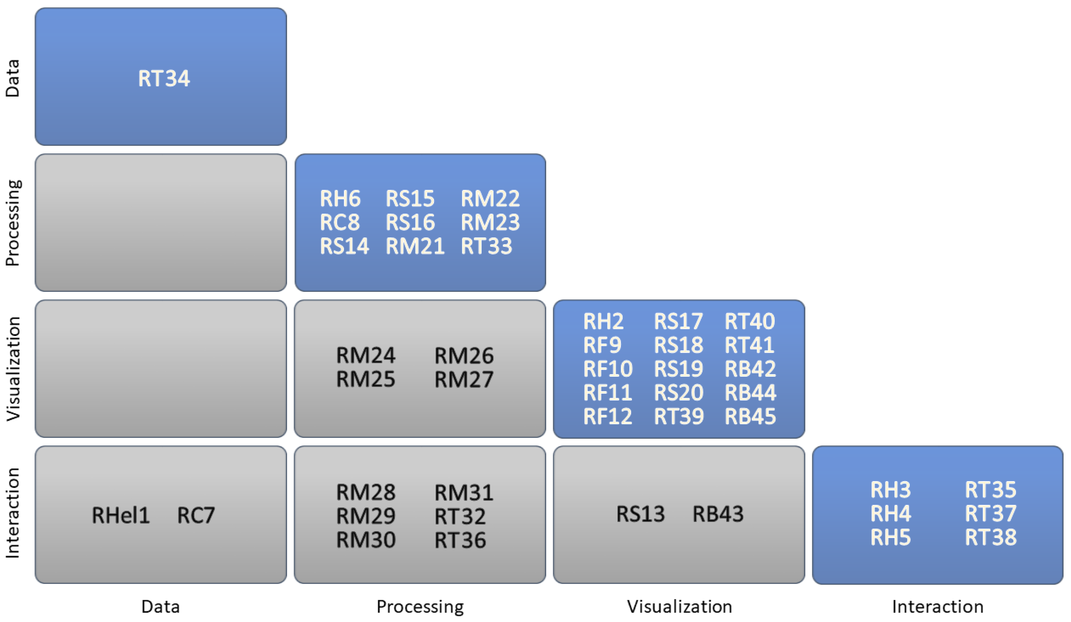
  • Data requirements concerning aspects from the ingestion and subdivision of the data, to prioritization and aggregation strategies for data in a PVA solution;
  • Processing requirements dealing with all aspects from the progressive implementation of the computation to its execution and control;
  • Visualization requirements regarding all aspects from visual feedback about the running process to the dynamic presentation of the incremental outcome;
  • Interaction requirements including all aspects from meeting human time constraints to providing structured interaction with the process.
The requirements in the literature address either one of these subjects exclusively, or they deal with the interplay of two phases. Figure 2 gives a summary of this relation between requirements and the different subjects to which they refer. Note that we list the requirements in the spirit in which they were introduced by their respective authors. For example, R S16 “Allow users to ignore irrelevant subspaces” was introduced by Stolper et al. [1] (Section 4.3), specifically as a requirement for the processing, or for the “analytics components” as they term it.
While we could easily see this requirement to also relate to the visualization in which the irrelevant subspaces must be identified, to the interaction that must provide some means to select them, and to the data handling that must ultimately be able to filter them out—we nevertheless placed it solely under processing, as it was originally intended. This makes sense, as for example, Stolper et al., also define another requirement R S20 that addresses the need for suitable visual interfaces to specify those irrelevant subspaces.

5.2. User-Driven Characterization

PVA requirements serve two general functions: There are those that provide PVA benefits to ensure that PVA’s advantages over MVA are available in a PVA solution. And there are those that address PVA challenges to ensure that the complications incurred by PVA can be handled. In the following, we discuss the PVA requirements with respect to the functions they provide to the PVA user, and we distill their main points into high-level recommendations.

5.2.1. Requirements for Providing PVA Benefits

The fundamental requirement for being able to provide PVA benefits at all is to use an algorithmic procedure that yields a sequence of results, as for example online algorithms do ( R T33). Yet to produce clear and strong advantages over MVA, the sequence of results must also be made accessible in suitable ways. This section summarizes the requirements for providing such ways.
Provide early partial results
There are three ingredients to providing useful early partial results: their immediacy, their significance, and their actionability.
Immediacy: The whole idea of early partial results is that they are provided promptly, which usually means that t Response must respect human time constants ( R T32), as they are listed under Section 4.1. Otherwise, the PVA process will be perceived as lagging or stalling. To ensure immediacy, PVA systems should be designed to start computations immediately after being invoked by the user ( R T35). They can also employ the aforementioned adaptive sampling mechanisms to ensure that only as much data as there is time for gets processed ( R T34).
Significance: A partial result, as early as it may be delivered, is only useful if it shows what the analyst needs to see. This notion is captured by various concepts, such as meaningfulness, interestingness, and relevance:
  • Meaningfulness ( R S14): Partial results should reflect the overall result by coming in the same format (sometimes called structure preservance R M24) and be appropriate to be taken in by a human analyst.
  • Interestingness ( R Hel1, R S15, R M29): Partial results are of no use, if those parts of the data, which interest the analyst most, get processed and shown last. Hence, it is important to be able to prioritize data and process it in order of decreasing interestingness.
  • Relevance ( R S16): Some parts of the data may not only be of lesser interest to the user, but actually be entirely irrelevant to the analysis task at hand. Being able to exclude irrelevant data from processing can further streamline the creation of useful partial results by making it faster and less cluttered.
As interestingness and relevance are highly user-dependent, it is further necessary to provide a suitable user interface to specify those notions ( R S20).
Actionability: In addition to having a significant and early partial result, the analyst must also be able to act upon it. Hence, the literature stresses the point that early partial results should already provide full interactivity ( R H5). This way, analysts can interact with them as they would interact with the completed result. In addition, a PVA system should allow analysts to perform an early cancellation of the running process ( R M28), if they perceive the early partial results as inadequate for their analytical needs.
Recommendation I:To provide early partial results—i.e., to establish t Response —first processing results should be delivered promptly, while maintaining their significance and interactivity.
Provide mature partial results
While mature partial results “inherit” the basic characteristics of early partial results of being significant and interactive, providing them is not so much a question of undercutting a particular time constraint. Instead, it is more about establishing trust in the still incomplete results, so that the analyst is comfortable to start the visual analysis early. For this, the core concern is to communicate the inherent uncertainty of the partial results, as well as the uncertainty of the computational process.
Uncertainty of the results: To judge how trustworthy a partial result is and thus how trustworthy any first observations are, it is of principal importance to communicate the uncertainty ( R M26). Uncertainty displays can range from minimally invasive measures, such as adding confidence bounds [8], to switching out the entire visualization for binned alternatives that prevent micro readings in still uncertain areas of the plot [7] (Section 2.4.3). For a simpler communication, the results’ uncertainty can also be condensed into numerical aggregates or quality metrics ( R M25).
Uncertainty of the process: Uncertainty is not only a characteristic of the partial result, but also of the process that generated it. As uncertainties in the computations may influence the trustworthiness of the results without being directly quantifiable, it is of equal importance to inform analysts about them ( R T41). Such provenance information can stretch from traits of the data preprocessing—i.e., the currently used sampling strategy, to the algorithmic parameters and any simplifications made during the process ( R M27).
Recommendation II:To provide mature partial results—i.e., to establish t Reliable —the inherent uncertainty of the partial results and of the progressive computation should be communicated truthfully and comprehensively for judging the results’ trustworthiness.
Provide definitive partial results
In contrast to mature partial results, definitive partial results are already quite certain and thus trustworthy. For them, it is not the uncertainty the analyst has to judge, but the stability of this state—i.e., is a seemingly good result already stable enough to be used in place of the final result? Or is it just a local optimum or an accidentally good outlier produced by a fluctuating computation that is not yet backed up by enough data chunks or iterations to be deemed stable? Hence, definitive partial results require not so much judging the individual partial result, but the computational process as whole. Indicators to inform this judgement are the process’ state and its progress.
State of the process: The analyst should be able to discern the aliveness of a process—i.e., whether a current result is no longer visibly changing, because the result is actually stable, or because the process is stalling due to a deadlock or a lost connection ( R M21).
Progress of the process: It can also be beneficial for the analyst to know how much processing has been done overall, either in absolute or relative terms ( R M22, R M23). Another way to indicate progress is to convey an estimated time to completion ( R T40). In some cases, the complete result may not be that far out and analysts may be willing to wait another minute for it, but not hours.
Note that prioritizing data ( R Hel1, R S15, R M29) or even having the user specify the data samples ( R C7) is also important for providing definitive partial results: it does not only allow seeing the interesting data first, but it also ensures that after a certain point only uninteresting data remains and the analysis can be completed early.
Recommendation III:To provide definitive partial results—i.e., to establish t Stable —the process’ state and progress should be communicated for judging its aliveness, convergence, and time of completion.
Provide a succession of results
The main requirement for being able to observe and influence the evolution of results is the use of suitable visualizations ( R T39) that lend themselves to being dynamically updated. In general, PVA tends to more generic visualizations than task-specific ones, trying to offer a visual representation that can be used for most tasks ( R F10); with scatterplots and heatmaps being popular choices in this regard. This is only logical, as visualizations in PVA are generated over time and quickly switching between different special-purpose visualizations according to different tasks is not an option, as the progression would have to start anew. Aside from these basic considerations, dynamic visualizations should further provide adequate means for monitoring the succession and for steering the succession.
Monitoring the succession: When observing the running process, it is paramount to not only have an expressive visual representation of the data and any associated uncertainties, but also of the amount of change in between updates. As a guiding principle, we want the change in the visualization to be proportional to the change in the underlying data ( R F11). Otherwise, we might see change where there is none and vice versa. The literature also points out the importance of supporting various monitoring tasks, such as spotting general changes with each update ( R H2, R S18), or tracking specific items of interest across multiple updates ( R H6).
Steering the succession: In some cases, it may be necessary to pause the progression on demand in order to inspect a particularly complex update. This is usually supported via pause/play mechanisms ( R H3, R T36), with which users are familiar from animated visualizations and video playback. In addition, it may also be of interest to change the time span between updates, e.g., by adapting the step-size or chunk-size of the progression ( R T36). More sophisticated modifications of the running process usually involve manual adjustments of intermediate results that are then used as input for the next processing step ( R M30)—e.g., to “help along” a clustering or a network layout.
Recommendation IV:To provide a succession of partial results, visualizations with change-proportional updates should be used together with interaction mechanisms for steering the progression dynamics and their visual representation.

5.2.2. Requirements for Mitigating PVA Challenges

Being able to start and complete analyses early by working in parallel with the computation requires additional efforts for monitoring and steering the computational process. While the last section discussed how to provide the benefits of making PVA accessible to the user, this section discusses the challenges of doing so and points out requirements that are aimed at reducing or even solving them.
Support the parametrization of the progression
A fundamental precondition to allow sensible parametrization of the progression is stated by R C8, which basically demands a decoupling of data and process parameters—i.e., changes to how the data are sampled should not incur changes on how the algorithm behaves and vice versa. If that requirement is not fulfilled, as for example, different algorithms are chosen depending on the size of the data chunks, seemingly simple parameter changes can yield unpredictable consequences. This precondition is necessary for both, interactive and automated parameter changes.
Interactive parameter changes: Turkay et al. [7] (Section 4.1.3) have observed that PVA users tend to be quite preoccupied with manual parameter changes—in particular in multi-view setups. To make manual parameter adjustments in an informed manner, one can employ multiple consecutive executions of the same progressive computation ( R M31). By using different parameters for each, their early partial results can be compared and the most promising can be chosen for continued processing.
Automated parameter changes: It is also possible to use adaptive mechanisms for auto-adjusting the parameters to match external constraints, such as a desired response time ( R T34). Such an automated parameter adjustment can not only be helpful to cope with input data of varying complexity, but also help to keep the user’s attention on the data analysis instead of being distracted by the multitude of PVA parameters and options ( R H4, R S13).
Recommendation V:To support the parametrization of PVA, changes to process and data parameters should yield predictable results that lend themselves to interactive and adaptive parametrization.
Support judging partial results
Not yet having the final result to compare with, it is extremely challenging to estimate the uncertainty of the currently shown partial result (how bad it still is) or its quality (how good it already is) [43]. Making the call of when a visualization is good enough to start and finish its analysis remains highly subjective, differing among analysts even when pursuing the same task on the same data [7] (Section 4.1.3). For reducing the cognitive efforts of taking in additional uncertainty information, the literature emphasizes the importance of minimizing the added visual complexity and of its consistent display across views.
Minimize added visual complexity: Communicating the uncertainty in addition to the currently shown result puts extra complexity in the visualization. If possible, this extra information should be rendered as an unobtrusive visual cue, adding minimal complexity to the base visualization and thus easing its interpretation ( R F9). Furthermore, these cues should use a distinct representation from the base visualization, so as not to add visual noise ( R F12). Error bars for column charts are a good example for both: While also using the height to encode the uncertainty value, they do not use the same column representation, which could have been confused with the columns from the base representation. Instead they only consist of a few extra lines per column that grow less pronounced as the uncertainty decreases.
Consistency across views: In multi-view setups, uncertainty should be displayed in a consistent fashion for all views ( R B45). Consistency does not only relate to using similar visual uncertainty representations across different views. It also concerns the effect of different views reaching stability at different points during the progression. Having a partial result that is apparently stable in one view and still changing in another is confusing to the user, which is why such discrepancies need to be taken into account ( R T37). One way of doing so is to compute the uncertainty in a global manner and to display it in a dedicated view as a summary statistic over all views.
Recommendation VI:To support judging partial results, their uncertainty should be visualized in a way that minimizes added visual complexity and ensures consistency across views.
Support monitoring the succession of results
To help observing the running progression, it is common to provide two modes ( R B43): a monitoring mode with continuously updating, dynamic views ( R H6) and an exploration mode with static views that only update on demand ( R S19). Both modes require different kinds of support for monitoring the progression: the dynamic views should be stabilized to maintain user orientation and the static views should incorporate additional dynamic features to indicate new results.
Stabilizing dynamic views: The main challenge of a “live” display of the progression is that constant changes of the view make it hard to keep one’s orientation, as the layout still moves data points around or simply adjusts the color scale as new values are added. While in some sense, these changes are representative of the progression, view changes still need to be limited ( R S17), as otherwise the animated view is nothing more than a flickering of seemingly unconnected partial results. A common way of doing this is by using visual anchors ( R B44) that introduce more stable landmarks in the view to provide a frame of reference for the analyst’s mental map. For example, in online dynamic graph drawing, this is done by assigning so-called pinning weights to central nodes, keeping them in place while the layout around them changes [44] (Section 4.1).
Dynamic features in static views: In case of static views, it is still important to convey the ongoing progression, so that the analysts know if the view they are currently working on is outdated and requires an update on demand. Some PVA systems use a global highlighting of the UI elements that are used for updating on demand—e.g., a “cautionary yellow background” to indicate that new results are available [28] (Section 3.2). Others provide more detail, for example by dynamically adding visual cues directly into the static view to mark those regions where new results are waiting to be incorporated [1] (Section 5.3). For the special case of asynchronous updates—i.e., updates that come in a different order than they were triggered—a color-coding of visual changes has been proposed to aid users in maintaining an overview of the succession [45].
Recommendation VII:To support monitoring the succession of results, the visualization should ensure stability for constantly changing dynamic views and embed dynamic features in fixed views.
Support steering the progression
Steering the progression adds onto the challenge of monitoring, as it not only implies that the analysts understand from the monitoring what is currently going on, but also know how to tune it to better comply with their expectations. Essential requirements for such a steering are that the analyst has general information about the computational process to know what to change, and gets immediate feedback on the changes to know how much to change it.
Information about the computational process: It is hard to steer a computational process that is a mere black box to the analyst. While it helps with the parametrization if this black box behaves deterministically ( R C8), for actually steering it by switching algorithms or excluding certain parts of the data, more information is needed. To support the steering, provenance information should be shown that detail the current computational pipeline ( R B42) and its current parametrization ( R M27).
Immediate feedback on made changes: Steering the progression in a particular direction by prioritizing certain data or adjusting algorithmic modules of the pipeline requires the analysts to see the effects of their changes to further fine-tune their adjustments. On one hand, this relates back to R T32 and R T35, which require swift responses without delays. On the other hand, this also means that the analysts must be able to observe any, possibly minor, effects in the output due to their steering of the process. Yet for more complex changes that involve adjustments of many intricate UI controls at the same time, this is hard to do in parallel. In these cases, structured interaction sequences ( R T38) can help to lessen the burden of the interactive steering and to be able to better focus on observing its output. These sequences automate low-level interactions, such as moving sliders across a particular interval or brushing/selecting data in certain regions.
Recommendation VIII:To support steering the progression, PVA systems should make the current processing pipeline explicit and employ mechanisms that reduce the interaction costs of steering as well as of reverting back to previous configurations.
Support handling fluctuating progressions
Fluctuations are another reason for distractions and interference with the analysis flow, which is to be avoided ( R H4, R S13). They can be induced by all aspects of visual analytics (cf. Section 5.1): by the data, by the computational process, by the visualization, and by the interaction.
Data-induced fluctuations: Fluctuations can originate from data chunks with a skewed data distribution that is not representative of the overall distribution in the dataset [46]. This happens when employing an inadequate sampling technique, but can in particular be observed when performing no sampling at all and simply partitioning the data as is. One solution is to randomize the data in a preprocess before loading it into the PVA system [19] (Section 4). This simple, yet effective solution is suited for scenarios in which one does not have access to the source of a PVA system and cannot add improved sampling functionality to it. Note that the opposite approach of sorting the data according to one’s own prioritization strategy can likewise be employed for PVA systems that do not support this.
Computational fluctuations: A common source for such fluctuations is the inclusion of random displacements in the computation to escape local optima. For example, in some computational approaches, such as genetic algorithms, random elements are an essential part of the principal approach and cannot be eliminated or reduced. A generic way of handling highly fluctuating processes and enforcing their gradual stabilization is to employ simulated annealing [47]. It uses a cooling factor to gradually limit changes as the results become better, but not necessarily more stable.
Visual fluctuations: Visualizations with absolute positioning that use the Euclidean space as a fixed frame of reference—e.g., scatterplots—remain reasonably stable unless the data items themselves move around. Yet for example, in case of network diagrams, relative positioning is used that places data items (nodes) in relation to each other. Such a relative positioning is prone to change with every added data item, and it is thus not surprising that the idea of simulated annealing has also been transferred to network visualizations [48] (Chaper 12.2). If fluctuations cannot be avoided, it is common practice to at least try to smoothly animate between successive updates using animated transitions [7] (Section 2.4.1) or staged animations [19] (Section 4.2).
Interaction-induced fluctuations: Interactions, such as reparametrizing or steering the process, are one of the main causes of discontinuities in the progression. The literature notes that interactions should take fluctuations into account ( R T37). Turkay et al. [7] (Section 2.3.2), suggest using structured interaction sequences ( R T38) to ensure a steady parameter changes without the intermediate discontinuities introduced by manual adjustments of sliders or brushes.
Recommendation IX:To handle fluctuations, these should be reduced by proper data sampling, by enforcing process stability, by using absolute positioning and animation, and by steadying interactions.

6. A Use Case Scenario

PVA is used for scenarios as diverse as designing neural networks [49] and pattern discovery in categorical data [50]. Each of these different scenarios has a different reason for using PVA and thus its very own take on how to concretely realize PVA. There exists no standard approach to implementing a PVA solution, as each real world PVA scenario rarely requires different PVA benefits and needs to handle different PVA challenges, depending on which flavor of PVA it uses (e.g., data chunking vs. process chunking). Hence, depending on the scenario at hand, different PVA solutions may employ a different subset of the proposed recommendations.
This section exemplifies this aspect by discussing a concrete use case in the context of our PVA characterization. It shows how the respective recommendations are reflected in the design of the resulting PVA system, illustrating how our characterization and recommendations can be used to inform the design of new PVA solutions, as well as to describe existing ones. In the following, we outline the specific setting of the scenario, position it in our PVA characterization, and detail the recommendations we followed to yield our PVA solution.

6.1. The Visual Analysis Setting

The use case at hand is taken from Angelini et al. [32]. It supports explorative decision making for marketing strategies of Telecom Italia Mobile (TIM). It seeks to find a subset of the 110 Italian provinces that leads to an optimal Return of Investment (RoI) as captured by a given objective function. This subset is iteratively derived in three steps:
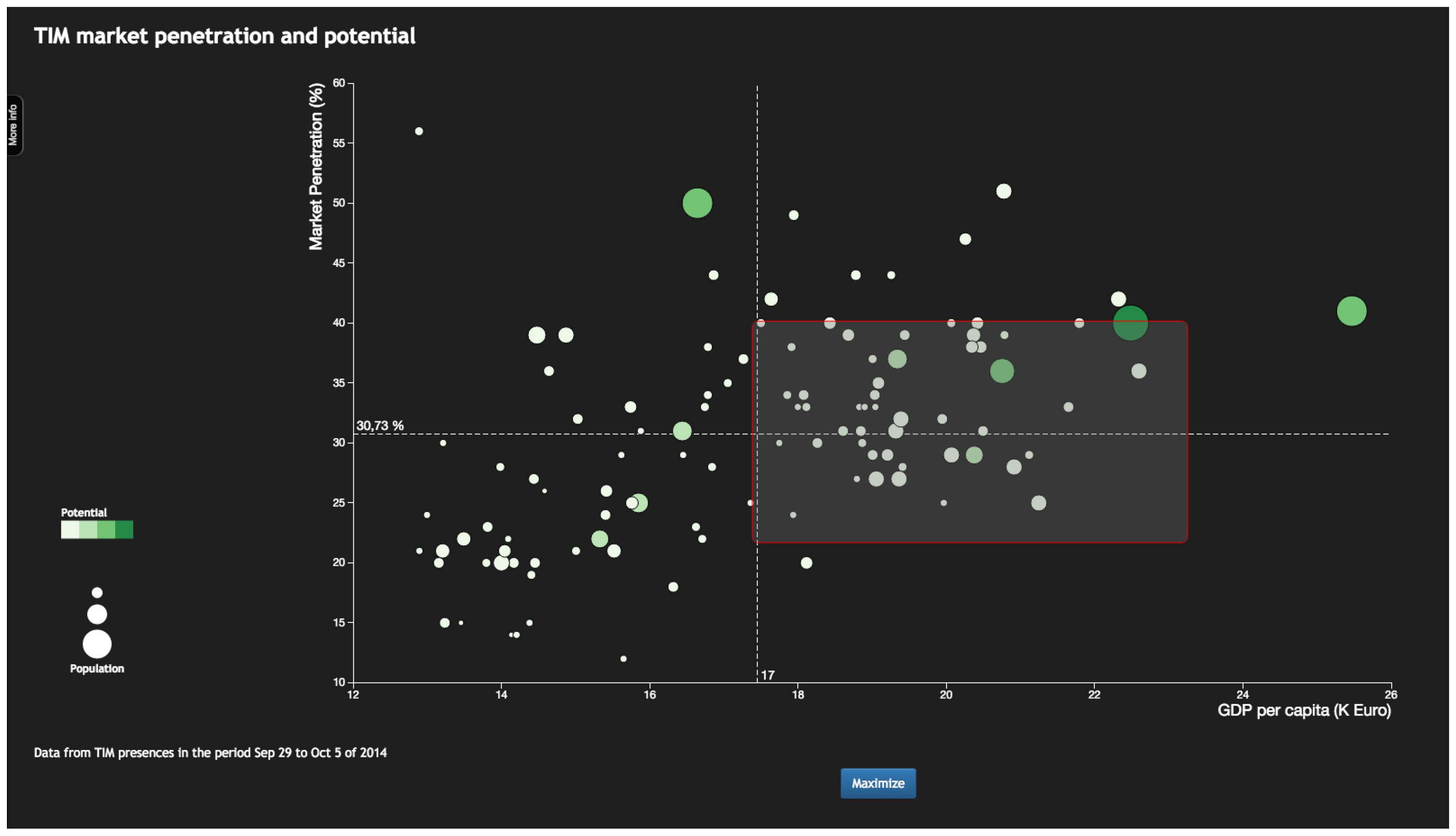
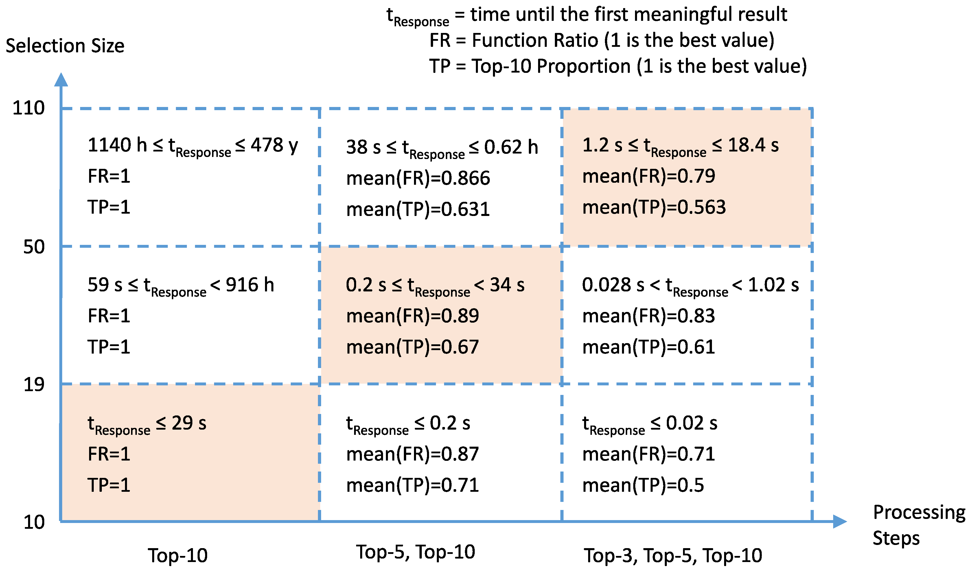
  • The analyst selects 30 to 50 candidate provinces in a scatterplot. This scatterplot displays the provinces according to numerical properties that will likely have an influence on the success of the marketing campaign—e.g., market penetration and average income as shown in Figure 3.
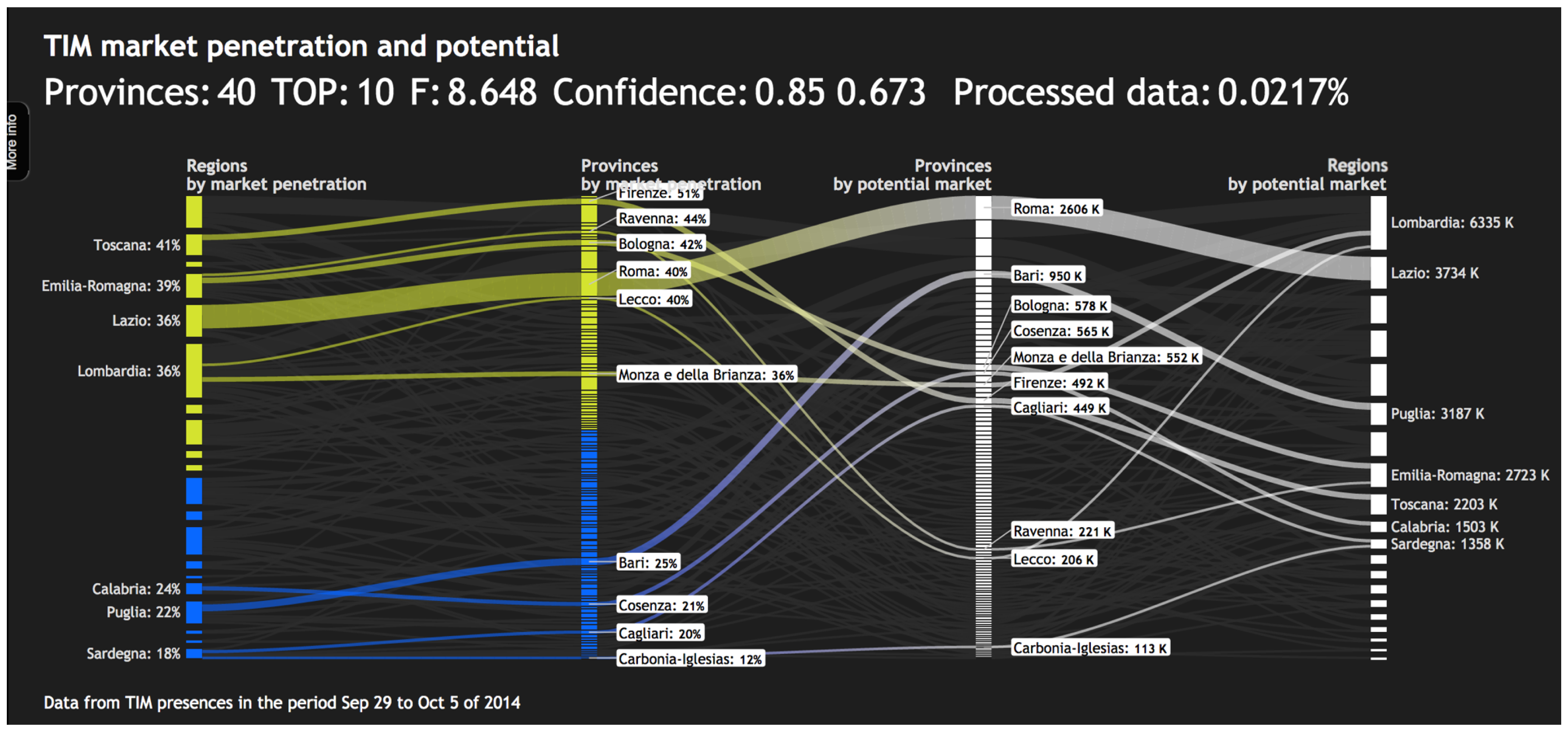
  • Among those candidate provinces, a Top-10 subset is computed that maximizes the objective function. The subset is displayed in a Sankey diagram, which allows the user to explore the numeric properties of these provinces as well as their relation to the provinces not included in the Top-10—see Figure 4.
  • Depending on the interactive assessment of the current set of Top-10 provinces, the analyst can either go back to the scatterplot to choose a different candidate set, or conclude the analysis with the current result and launch the marketing campaign in those ten provinces.
In the following assessment of this use case, we focus on the second step, as this step incorporates the progressive computation of the Top-10 provinces. The Sankey diagram used to visualize the (intermediate) results from this computation encodes the flow between two data facets: the market penetration (percentage of population in possession of a SIM card in the concerned territories) shown by the two leftmost axes, and the potential market (difference between the population index and the absolute value of the potential market) shown by the two rightmost axes. The two axes for each data facet encode the data on two different geospatial aggregation levels—regions and provinces. Ribbons between the middle axes connect the provinces to their counterparts on the left/right, and ribbons to the outer axes connect the provinces to the regions they belong to. As the width of the ribbons is proportionally sized to the population of the corresponding regions and provinces, they convey visually how each of them contributes to the overall RoI value.

6.2. Characterization as a PVA Scenario

Reason for using PVA: Finding the Top-10 is a combinatorial optimization problem for which no better solution exists than testing all possible combinations of 10 provinces out of the selected candidate set. Computing the Top-10 on all 110 provinces and assuming we could test 3000 combinations in a second (actual throughput on an Intel Core i7 with 3.1 GHz), getting the exact result would require around 500 years, which is certainly quasi-indefinite. Under the same assumption, given a candidate set of only 40 provinces this computation would still require 75 h. While this may still be doable, t Complete lies well beyond the expected task completion time of around 10 s, effectively hindering a fluent analysis.
Benefits of using PVA: The iterative assessment of the result for different, manually tested and refined candidate sets poses clear time constraints on the computation of the Top-10 provinces. To keep the analyst engaged in a fluid back and forth between scatterplot and Sankey diagram, we need to provide a result within a time frame of at most 30 s. PVA can be used to achieve this by producing early partial results within such an acceptable time span, which are then further refined into mature partial results while the analyst already starts exploring.
Challenges of using PVA: Using PVA to yield a swift first response from the computation creates several challenges that our PVA design has to address. The foremost challenge is the inexact nature of the partial results and the analyst’s need to judge them. In addition, the generated partial results are likely to fluctuate, so that a province might disappear from the Top-10 only to be reintroduced later. Finally, the parametrization of the data partitioning affects the runtime until the first result is produced. Choosing it inappropriately can easily result in extremely long wait times even for the first early partial result.

6.3. A Solution Design following the PVA Recommendations

The above characterization makes it obvious that this PVA scenario puts emphasis on some aspects, while neglecting others. Our telecom marketers are not interested in definite partial results or even the final result, as it is not necessary to find the best possible Top-10 set of provinces that improves the RoI of an already mature Top-10 by a few digits after the decimal point. We define the maturity of an intermediate Top-10 result in terms of the inherent uncertainty of the process, which we infer from a metric that captures how many out of the 10 optimal provinces are already included in the current Top-10 (see below for its computation). Overall, the users are not much interested in the process of the computation itself and have no concern for monitoring the succession of results, let alone steering it. Hence, our PVA solution, shown in Figure 4, follows the recommendations relating to the PVA benefits and challenges identified in Section 6.2.
Providing PVA Benefits: A prerequisite of any PVA solution is to employ a procedure that produces a stream of intermediate results. As a general approach, our PVA solution samples subsets of increasing size from the candidate set, computes their Top-10, and replaces the current best solution with the new one, if the newly produced Top-10 performs better with respect to the objective function.
Recommendation I: While this general approach could be used to deliver a prompt early result, this result would most likely be far from significant and worth to be explored, as it initially only covers a small subset of the candidate set. Hence, we employ a slightly different strategy for the first partial result that ensures significance by covering the whole candidate set, while maintaining acceptable response times: We divide the candidate set in two disjoint subsets of equal size, independently compute their Top-5 provinces, and merge them into the very first Top-10 shown in the interactive Sankey diagram. Subdivisions into even more subsets (e.g., Top-3) are also possible, depending on the size of the candidate set and the desired t Response .
Recommendation II: To provide means for estimating the inherent uncertainty of the current partial result and of the progressive computation, we have implemented an adaptive strategy, sampling the whole design space with different selection sizes and process granularities, to find suitable trade-offs. This strategy is implemented defining three intervals for the process granularity and three intervals for the selection size, effectively obtaining nine possible configurations as their pairwise combinations (see Figure 5). For each of these nine possible configurations, we collected and averaged two measures:
T o p - 10   P r o p o r t i o n ( T P ) = E s t i m a t e d   T o p - 10 r e a l   T o p - 10 10    F u n c t i o n   R a t i o ( F R ) = E s t i m a t e d   f u n c t i o n o p t i m a l   v a l u e
These measures are used to provide the user with two confidence indicators: The T P value denotes the stability of the current result. It can be read as the fraction of provinces of the current Top-10 that will most likely also be part of the final Top-10. The F R value denotes how good the current value of the objective function is compared to the probable optimum. As neither the real Top-10 nor the optimal value can actually be obtained for large n, we use approximations. For example, for the real Top-10, we use an average of a number feasible Top-10s computed on random provinces subsets, e.g., ( 40 10 ) , ( 40 5 ) , and ( 40 3 ) .
In addition, the percentage of processed data shows how many out of all possible province combinations have been tested so far. Its basic idea is to put the confidence values TP and FR into context by indicating just how few combinations have been tested so far and how long it would thus take to be entirely certain. The analyst can then decide based on these data, whether it makes sense to wait for a longer time to improve the actual result.
Mitigating PVA Challenges: Our main design decision to counter the challenges was the use of a minimalistic visual interface that masks the complexity of the underlying computation and its parametrization. Its only visual feature is the Sankey diagram showing the current best result, while all other information is given in textual or numerical form to not distract the user and to keep possible fluctuations in the graphics to a minimum.
Recommendation V: The two parameters having most influence on t Response are the size of the candidate set and the number of subsets into which the candidate set is partitioned. As the candidate set is chosen by the user, we have no control over it. Based on the benchmarks from Figure 5, we use an adaptive parametrization for the number of subsets, which does not subdivide if the candidate set contains 19 provinces, subdivides into two subsets for anything between 19 and 50 provinces, and into three sets for 50 provinces. This way, we can guarantee t Response of 29 s, 34 s, and 18 s, respectively.
Recommendation VI: To minimize added visual complexity, our PVA solution shows the uncertainty of the current result only in numerical form. We make it easy to interpret this numerical uncertainty information by not just computing some abstract quality/error metrics, but actually providing indicators of how good the current solution already is (first confidence value) and what could still be gained by waiting for a better result (second confidence value).
Recommendation IX: While new results are continuously produced by our procedure, only results that are better than the current best result will update the view. This leads to the effect that view updates come irregularly and unforeseeably, and there is not much we can do about it. At least the analysts know that any update is an improvement over the current view and that they do not have to worry about having a good intermediate result being replaced by one that is worse. To smooth the visual changes resulting from the transition to an updated result, the Sankey diagram does not only show the current Top-10, but all candidate provinces. This way, provinces do not appear and disappear, but merely move up to join the Top-10 or down if excluded again. This movement is animated to help following the transition. To stabilize the interaction, the system automatically blocks the rendering of a new partial result if the user is interacting with the current one.

6.4. User Feedback

We conducted several informal tests with Telecom Italia Mobile users in order to collect feedback. The users were provided with the PVA solution and asked to explore the given scenario and propose the Top-10 they considered as best solution. Eventually during a following discussion users were asked for the confidence they have in their answers. Summarizing the obtained feedback, users appreciated to have progressively refining results on which they could immediately start the exploration process and form hypotheses. Nonetheless, we experienced different sensibilities to interpret confidence of the results and eventual exploration of alternatives. The users asked us to provide more nuanced insight in the magnitude of Top-10 changes. For example, they would like to see how big of an improvement to the RoI the changes have provided. This makes sense, as there may be a lot of changes, but if these only concern the lower ranks of the Top-10 with the Top-8 or Top-9 item being swapped out for minor RoI improvements, the result might already be stable enough to work with it.

7. Conclusions

With the PVA characterization and recommendations given in this paper, we have extracted the common aspects from a broad range of literature. Regardless of the very diverse areas from which these papers stem, the reasons for using PVA, the utilized benefits of PVA and the observed challenges are almost unifying factors among them. They only differ in the concrete requirements they state for dealing with them, with some PVA solutions striving to provide PVA benefits and counter PVA challenges on data level, while others go for the processing, visualization, or interaction. Yet even this diverse set of requirements has its common elements, which we subsumed as recommendations. Together, these aspects span the realm of PVA as it is currently described in the literature.
Going through the existing papers, we did not only obtain an overview of the research that has already been done in PVA. We also noticed aspects that have not yet been looked into and remain open questions for future research. In the light of all the requirements for designing PVA systems, one of the most pressing open question is once we have such a system, how to evaluate it? While current research conducts user studies on PVA approaches as if they are MVA approaches, recent work by Boukhelifa et al. [51] suggests that judging uncertain results introduces entirely new tasks, which should probably be reflected in PVA studies. So it might be time to work on a progressive task taxonomy to ensure that PVA systems are evaluated with appropriate tasks and criteria.
Another open point for research is to devise progressive analysis and visualization methods as building blocks to be used in PVA systems. This is by no means a simple task and adapting existing techniques to the PVA concept is a complex research question in its own regard, very similar to the problem of parallelizing existing algorithms for their distributed use. For some techniques, progressive variants have already been proposed – for example, for k-Means [52], MDS [53], t-SNE [54], Treemaps [55], and Parallel Coordinates [56,57]. Yet these are merely a tiny fraction of the analysis and visualization techniques our community are accustomed to use.
As a result of these open questions, this paper is neither a final treatment nor a complete systematization of the PVA concept. It is a snapshot of this particular research domain as of June 2018, which bundles and connects the various aspects and notions that have been discussed so far. We intend this snapshot to consolidate and converge research efforts in PVA, providing a common ground for scientific discussions and engineering decisions in this domain.

Author Contributions

The initial idea for this overview came from H.S. The abstract introductory process model used to describe the fundamentals of PVA in Section 2 was developed by H.-J.S. The PVA characterization in Section 4 and the collection of requirements and their abstraction into recommendations in Section 5 have been established jointly by all authors over the course of a week-long retreat in Rostock in 2017. The use case in Section 6 was provided by M.A. and G.S. The paper was prepared by G.S., H.-J.S. and M.A. incorporating critical feedback and editorial remarks provided by H.S. Overall, all authors have contributed equally to this paper.

Funding

This research received no external funding.

Acknowledgments

The authors are grateful to the anonymous reviewers for their helpful comments and suggestions, as well as to Christian Tominski for providing his critical opinion on many of the discussed aspects.

Conflicts of Interest

The authors declare no conflict of interest.

Abbreviations

The following abbreviations are used in this manuscript:
HCIHuman-Computer Interaction
IVAInstantaneous Visual Analytics
MDSMulti-Dimensional Scaling
MVAMonolithic Visual Analytics
PVAProgressive Visual Analytics
RoIReturn of Investment
SIMSubscriber Identity Module
SNEStochastic Neighbor Embedding
TIMTelecom Italia Mobile

Appendix A. List of requirements

Table A1. Requirements collected from the current body of literature on PVA.
RequirementDescriptionSource
R Hel1Process interesting data early, so users can get satisfactory results quickly, halt processing, and move on to their next requestHellerstein et al., 1999 (Preferential data delivery: online reordering)
R H2Enable monitoring the visualization and seeing what’s new each time a new increment of data is processed and loaded into the systemHetzler et al., 2005 (Section 3.1)
R H3Allow the explicit control of updates arrivalHetzler et al., 2005 (Section 3.2)
R H4Minimize the disruption to the analytic process flow and the interaction flowHetzler et al., 2005 (Section 3.2)
R H5Provide full interactivity for dynamic datasetsHetzler et al., 2005 (Section 3.3)
R H6Provide dynamic update featuresHetzler et al., 2005 (Section 3.4)
R C7Allow users to communicate progressive samples to the systemChandramouli et al., 2013 (Section 1.1)
R C8Allow efficient and deterministic query processing over progressive samples, without the system itself trying to reason about specific sampling strategies or confident estimationChandramouli et al., 2013 (Section 1.1)
R F9Uncertainty visualization should be easy to interpretFerreira et al., 2014 (Design Goals)
R F10Visualizations should be consistent across tasksFerreira et al., 2014 (Design Goals)
R F11Maintain spatial stability of visualizations across sample sizeFerreira et al., 2014 (Design Goals)
R F12Minimize visual noiseFerreira et al., 2014 (Design Goals)
R S13Managing the partial results in the visual interface should not interfere with the user’s cognitive workflowStolper et al., 2014 (Section 1)
R S14Produce increasingly meaningful partial resultsStolper et al., 2014 (Section 4.3)
R S15Allow users to focus the algorithm to subspaces of interestStolper et al., 2014 (Section 4.3)
R S16Allow users to ignore irrelevant subspacesStolper et al., 2014 (Section 4.3)
R S17Minimize distractions by not changing views excessivelyStolper et al., 2014 (Section 4.3)
R S18Provide cues to indicate where new results have been found by analyticsStolper et al., 2014 (Section 4.3)
R S19Support an on-demand refresh when analysts are ready to explore the latest resultsStolper et al., 2014 (Section 4.3)
R S20Provide an interface to specify where analytics should focus, as well as the portions of the problem space that should be ignoredStolper et al., 2014 (Section 4.3)
R M21Provide feedback on the aliveness of the executionMühlbacher et al., 2014 (Section 3.1)
R M22Provide feedback on the absolute progress of the executionMühlbacher et al., 2014 (Section 3.1)
R M23Provide feedback on the relative progress of the executionMühlbacher et al., 2014 (Section 3.1)
R M24Generate structure-preserving intermediate resultsMühlbacher et al., 2014 (Section 3.2)
R M25Provide aggregated informationMühlbacher et al., 2014 (Section 3.2)
R M26Provide feedback on the uncertainty of a resultMühlbacher et al., 2014 (Section 3.2)
R M27Provide provenance information, including any meta-information concerning simplifications made for generating a partial resultMühlbacher et al., 2014 (Section 3.2)
R M28Allow for execution control by cancellationMühlbacher et al., 2014 (Section 3.3)
R M29Allow altering the sequence of intermediate results through prioritizationMühlbacher et al., 2014 (Section 3.3)
R M30Provide inner result control for steering a single ongoing computation before it eventually returns a final resultMühlbacher et al., 2014 (Section 3.4)
R M31Provide outer result control to generate a result from multiple consecutive executions of a computationMühlbacher et al., 2014 (Section 3.4)
R T32Employ human time constantsTurkay et al., 2017 (Section 2.1, DR1)
R T33Employ online learning algorithmsTurkay et al., 2017 (Section 2.2, DR2)
R T34Employ an adaptive sampling mechanism (convergence & temporal constraints)Turkay et al., 2017 (Section 2.2.2, DR3)
R T35Facilitate the immediate initiation of computations after user interactionTurkay et al., 2017 (Section 2.3.1, DR4)
R T36Provide interaction mechanisms enabling management of the progressionTurkay et al., 2017 (Section 2.3.1, DR5)
R T37Design interaction taking into account fluctuationsTurkay et al., 2017 (Section 2.3.1, DR6)
R T38Provide interaction mechanisms to define structured investigation sequenceTurkay et al., 2017 (Section 2.3.2, DR7)
R T39Support the interpretation of the evolution of the results through suitable visualizationsTurkay et al., 2017 (Section 2.4.1, DR8)
R T40Inform analysts on the progress of computations and indicate the time-to-completionTurkay et al., 2017 (Section 2.4.3, DR9)
R T41Inform analysts on the uncertainty in the computations and the way the computations developTurkay et al., 2017 (Section 2.4.3, DR10)
R B42Show the analysis pipelineBadam et al., 2017 (Section 7.3)
R B43Support monitoring mode and exploration modeBadam et al., 2017 (Section 7.3)
R B44Provide similarity anchorsBadam et al., 2017 (Section 7.3)
R B45Use consistently visualized quality measuresBadam et al., 2017 (Section 7.3)

References

  1. Stolper, C.; Perer, A.; Gotz, D. Progressive visual analytics: User-driven visual exploration of in-progress analytics. IEEE Trans. Vis. Comput. Graph. 2014, 20, 1653–1662. [Google Scholar] [CrossRef] [PubMed]
  2. Fekete, J.D.; Primet, R. Progressive Analytics: A Computation Paradigm for Exploratory Data Analysis. arXiv, 2016; arXiv:1607.05162. [Google Scholar]
  3. Schulz, H.J.; Angelini, M.; Santucci, G.; Schumann, H. An Enhanced Visualization Process Model for Incremental Visualization. IEEE Trans. Vis. Comput. Graph. 2016, 22, 1830–1842. [Google Scholar] [CrossRef] [PubMed]
  4. Glueck, M.; Khan, A.; Wigdor, D. Dive in! Enabling progressive loading for real-time navigation of data visualizations. In Proceedings of the SIGCHI Conference on Human Factors in Computing Systems (CHI), Toronto, ON, Canada, 26 April–1 May 2014; Schmidt, A., Grossman, T., Eds.; ACM: New York, NY, USA, 2014; pp. 561–570. [Google Scholar] [CrossRef]
  5. Mühlbacher, T.; Piringer, H.; Gratzl, S.; Sedlmair, M.; Streit, M. Opening the black box: Strategies for increased user involvement in existing algorithm implementations. IEEE Trans. Vis. Comput. Graph. 2014, 20, 1643–1652. [Google Scholar] [CrossRef] [PubMed]
  6. Rosenbaum, R.; Schumann, H. Progressive refinement: more than a means to overcome limited bandwidth. In Proceedings of the Conference on Visualization and Data Analysis (VDA), San Jose, CA, USA, 18–22 January 2009; Börner, K., Park, J., Eds.; SPIE: Bellingham, WA, USA, 2009; p. 72430I. [Google Scholar] [CrossRef]
  7. Turkay, C.; Kaya, E.; Balcisoy, S.; Hauser, H. Designing Progressive and Interactive Analytics Processes for High-Dimensional Data Analysis. IEEE Trans. Vis. Comput. Graph. 2017, 23, 131–140. [Google Scholar] [CrossRef] [PubMed]
  8. Fisher, D.; Popov, I.; Drucker, S.M.; Schraefel, M. Trust Me, I’m Partially Right: Incremental Visualization Lets Analysts Explore Large Datasets Faster. In Proceedings of the SIGCHI Conference on Human Factors in Computing Systems (CHI), Austin, TX, USA, 5–10 May 2012; Konstan, J.A., Chi, E.H., Höök, K., Eds.; ACM: New York, NY, USA, 2012; pp. 1673–1682. [Google Scholar] [CrossRef]
  9. Song, D.; Golin, E. Fine-grain visualization algorithms in dataflow environments. In Proceedings of the IEEE Conference on Visualization (VIS), San Jose, CA, USA, 25–29 October 1993; Nielson, G.M., Bergeron, D., Eds.; IEEE: Piscataway, NJ, USA, 1993; pp. 126–133. [Google Scholar] [CrossRef]
  10. Hellerstein, J.M.; Avnur, R.; Chou, A.; Hidber, C.; Olston, C.; Raman, V.; Roth, T.; Haas, P.J. Interactive Data Analysis: The Control Project. IEEE Comput. 1999, 32, 51–59. [Google Scholar] [CrossRef]
  11. Frey, S.; Sadlo, F.; Ma, K.L.; Ertl, T. Interactive Progressive Visualization with Space-Time Error Control. IEEE Trans. Vis. Comput. Graph. 2014, 20, 2397–2406. [Google Scholar] [CrossRef] [PubMed] [Green Version]
  12. Kim, H.; Choo, J.; Lee, C.; Lee, H.; Reddy, C.K.; Park, H. PIVE: Per-Iteration Visualization Environment for Real-time Interactions with Dimension Reduction and Clustering. In Proceedings of the AAAI Conference on Artificial Intelligence, San Francisco, CA, USA, 1–9 February 2017; Singh, S., Markovitch, S., Eds.; AAAI: Menlo Park, CA, USA, 2017; pp. 1001–1009. [Google Scholar]
  13. Moritz, D.; Fisher, D.; Ding, B.; Wang, C. Trust, but Verify: Optimistic Visualizations of Approximate Queries for Exploring Big Data. In Proceedings of the SIGCHI Conference on Human Factors in Computing Systems (CHI), Denver, CO, USA, 6–11 May 2017; Lampe, C., Schraefel, M.C., Hourcade, J.P., Appert, C., Wigdor, D., Eds.; ACM: New York, NY, USA, 2017; pp. 2904–2915. [Google Scholar] [CrossRef]
  14. Kwon, B.C.; Verma, J.; Haas, P.J.; Demiralp, Ç. Sampling for Scalable Visual Analytics. IEEE Comput. Graph. Appl. 2017, 37, 100–108. [Google Scholar] [CrossRef] [PubMed]
  15. Zgraggen, E.; Galakatos, A.; Crotty, A.; Fekete, J.D.; Kraska, T. How Progressive Visualizations Affect Exploratory Analysis. IEEE Trans. Vis. Comput. Graph. 2017, 23, 1977–1987. [Google Scholar] [CrossRef] [PubMed] [Green Version]
  16. Lins, L.; Klosowski, J.T.; Scheidegger, C. Nanocubes for Real-Time Exploration of Spatiotemporal Datasets. IEEE Trans. Vis. Comput. Graph. 2013, 19, 2456–2465. [Google Scholar] [CrossRef] [PubMed] [Green Version]
  17. Nocke, T.; Heyder, U.; Petri, S.; Vohland, K.; Wrobel, M.; Lucht, W. Visualization of Biosphere Changes in the Context of Climate Change. In Proceedings of the International Conference on IT and Climate Change (ITCC), Berlin, Germany, 25–26 September 2008; Wohlgemuth, V., Ed.; Trafo Wissenschaftsverlag: Berlin, Germany, 2009; pp. 29–36. [Google Scholar]
  18. Sacha, D.; Stoffel, A.; Stoffel, F.; Kwon, B.C.; Ellis, G.; Keim, D.A. Knowledge Generation Model for Visual Analytics. IEEE Trans. Vis. Comput. Graph. 2014, 20, 1604–1613. [Google Scholar] [CrossRef] [PubMed]
  19. Badam, S.K.; Elmqvist, N.; Fekete, J.D. Steering the Craft: UI Elements and Visualizations for Supporting Progressive Visual Analytics. Comput. Graph. Forum 2017, 36, 491–502. [Google Scholar] [CrossRef] [Green Version]
  20. Marai, G.E. Activity-Centered Domain Characterization for Problem-Driven Scientific Visualization. IEEE Trans. Vis. Comput. Graph. 2018, 24, 913–922. [Google Scholar] [CrossRef] [PubMed]
  21. Amar, R.A.; Stasko, J.T. Knowledge Precepts for Design and Evaluation of Information Visualizations. IEEE Trans. Vis. Comput. Graph. 2005, 11, 432–442. [Google Scholar] [CrossRef] [PubMed]
  22. Fink, A. Conducting Research Literature Reviews: From the Internet to Paper, 4th ed.; SAGE Publishing: Thousand Oaks, CA, USA, 2014. [Google Scholar]
  23. Hellerstein, J.M.; Haas, P.J.; Wang, H.J. Online Aggregation. SIGMOD Record 1997, 26, 171–181. [Google Scholar] [CrossRef]
  24. Ding, X.; Jin, H. Efficient and Progressive Algorithms for Distributed Skyline Queries over Uncertain Data. IEEE Trans. Knowl. Data Eng. 2012, 24, 1448–1462. [Google Scholar] [CrossRef]
  25. Chandramouli, B.; Goldstein, J.; Quamar, A. Scalable Progressive Analytics on Big Data in the Cloud. Proc. VLDB Endow. 2013, 6, 1726–1737. [Google Scholar] [CrossRef]
  26. Im, J.F.; Villegas, F.G.; McGuffin, M.J. VisReduce: Fast and responsive incremental information visualization of large datasets. In Proceedings of the IEEE International Conference on Big Data (BigData), Silicon Valley, CA, USA, 6–9 October 2013; Hu, X., Lin, T.Y., Raghavan, V., Wah, B., Baeza-Yates, R., Fox, G., Shahabi, C., Smith, M., Yang, Q., Ghani, R., et al., Eds.; IEEE: Piscataway, NJ, USA, 2013; pp. 25–32. [Google Scholar] [CrossRef]
  27. Procopio, M.; Scheidegger, C.; Wu, E.; Chang, R. Load-n-Go: Fast Approximate Join Visualizations That Improve Over Time. In Proceedings of the Workshop on Data Systems for Interactive Analysis (DSIA), Phoenix, AZ, USA, 1–2 October 2017. [Google Scholar]
  28. Hetzler, E.G.; Crow, V.L.; Payne, D.A.; Turner, A.E. Turning the bucket of text into a pipe. In Proceedings of the IEEE Symposium on Information Visualization (InfoVis), Minneapolis, MN, USA, 23–25 October 2005; Stasko, J., Ward, M.O., Eds.; IEEE: Piscataway, NJ, USA, 2005; pp. 89–94. [Google Scholar] [CrossRef]
  29. Wong, P.C.; Foote, H.; Adams, D.; Cowley, W.; Thomas, J. Dynamic visualization of transient data streams. In Proceedings of the IEEE Symposium on Information Visualization (InfoVis), Seattle, WA, USA, 20–21 October 2003; Munzner, T., North, S., Eds.; IEEE: Piscataway, NJ, USA, 2003; pp. 97–104. [Google Scholar] [CrossRef]
  30. García, I.; Casado, R.; Bouchachia, A. An Incremental Approach for Real-Time Big Data Visual Analytics. In Proceedings of the IEEE International Conference on Future Internet of Things and Cloud Workshops (FiCloudW), Vienna, Austria, 22–24 August 2016; Younas, M., Awan, I., Haddad, J.E., Eds.; IEEE: Piscataway, NJ, USA, 2016; pp. 177–182. [Google Scholar] [CrossRef] [Green Version]
  31. Crouser, R.J.; Franklin, L.; Cook, K. Rethinking Visual Analytics for Streaming Data Applications. IEEE Int. Comput. 2017, 21, 72–76. [Google Scholar] [CrossRef]
  32. Angelini, M.; Corriero, R.; Franceschi, F.; Geymonat, M.; Mirabelli, M.; Remondino, C.; Santucci, G.; Stabellini, B. A Visual Analytics System for Mobile Telecommunication Marketing Analysis. In Proceedings of the International EuroVis Workshop on Visual Analytics (EuroVA), Groningen, The Netherlands, 6–7 June 2016; Andrienko, N., Sedlmair, M., Eds.; Eurographics Association: Aire-la-Ville, Switzerland, 2016. [Google Scholar] [CrossRef]
  33. Elmqvist, N.; Vande Moere, A.; Jetter, H.C.; Cernea, D.; Reiterer, H.; Jankun-Kelly, T.J. Fluid interaction for information visualization. Inform. Vis. 2011, 10, 327–340. [Google Scholar] [CrossRef] [Green Version]
  34. Shneiderman, B. Response time and display rate in human performance with computers. ACM Comput. Surv. 1984, 16, 265–285. [Google Scholar] [CrossRef]
  35. Card, S.; Robertson, G.; Mackinlay, J. The information visualizer, an information workspace. In Proceedings of the SIGCHI Conference on Human Factors in Computing Systems (CHI), New Orleans, LA, USA, 27 April–2 May 1991; Robertson, S.P., Olson, G.M., Olson, J.S., Eds.; ACM: New York, NY, USA, 1991; pp. 181–188. [Google Scholar] [CrossRef]
  36. Liu, Z.; Heer, J. The Effects of Interactive Latency on Exploratory Visual Analysis. IEEE Trans. Vis. Comput. Graph. 2014, 20, 2122–2131. [Google Scholar] [CrossRef] [PubMed] [Green Version]
  37. Qu, H.; Zhou, H.; Wu, Y. Controllable and Progressive Edge Clustering for Large Networks. In Graph Drawing. GD 2006. Lecture Notes in Computer Science; Kaufmann, M., Wagner, D., Eds.; Springer: Berlin/Heidelberg, Germany, 2007; pp. 399–404. [Google Scholar] [CrossRef]
  38. Jo, J.; Seo, J.; Fekete, J.D. A Progressive k-d tree for Approximate k-Nearest Neighbors. In Proceedings of the Workshop on Data Systems for Interactive Analysis (DSIA), Phoenix, AZ, USA, 1–2 October 2017; Chang, R., Scheidegger, C., Fisher, D., Heer, J., Eds.; IEEE: Piscataway, NJ, USA, 2017; pp. 1–5. [Google Scholar] [CrossRef]
  39. Fisher, D. Big Data Exploration Requires Collaboration Between Visualization and Data Infrastructures. In Proceedings of the Workshop on Human-In-the-Loop Data Analytics (HILDA), San Francisco, CA, USA, 26 June–1 July 2016; Binnig, C., Fekete, A., Nandi, A., Eds.; ACM: New York, NY, USA, 2016; pp. 16:1–16:5. [Google Scholar] [CrossRef]
  40. Crotty, A.; Galakatos, A.; Zgraggen, E.; Binnig, C.; Kraska, T. The Case for Interactive Data Exploration Accelerators (IDEAs). In Proceedings of the Workshop on Human-In-the-Loop Data Analytics (HILDA), San Francisco, CA, USA, 26 June–1 July 2016; Binnig, C., Fekete, A., Nandi, A., Eds.; ACM: New York, NY, USA, 2016; pp. 11:1–11:6. [Google Scholar] [CrossRef]
  41. Angelini, M.; Santucci, G. On Visual Stability and Visual Consistency for Progressive Visual Analytics. In Proceedings of the International Conference on Information Visualization Theory and Applications (IVAPP), Porto, Portugal, 27 February–1 March 2017; Linsen, L., Telea, A., Braz, J., Eds.; SciTePress: Setúbal, Portugal, 2017; pp. 335–341. [Google Scholar] [CrossRef]
  42. Ferreira, N.; Fisher, D.; König, A.C. Sample-oriented task-driven visualizations: Allowing users to make better, more confident decisions. In Proceedings of the SIGCHI Conference on Human Factors in Computing Systems (CHI), Paris, France, 27 April–2 May 2014; Schmidt, A., Grossman, T., Eds.; ACM: New York, NY, USA, 2014; pp. 571–580. [Google Scholar] [CrossRef]
  43. Angelini, M.; Santucci, G. Modeling Incremental Visualizations. In Proceedings of the International EuroVis Workshop on Visual Analytics (EuroVA), Leipzig, Germany, 17–18 June 2013; Pohl, M., Schumann, H., Eds.; Eurographics Association: Aire-la-Ville, Switzerland, 2013; pp. 13–17. [Google Scholar] [CrossRef]
  44. Frishman, Y.; Tal, A. Online Dynamic Graph Drawing. IEEE Trans. Vis. Comput. Graph. 2008, 14, 727–740. [Google Scholar] [CrossRef] [PubMed] [Green Version]
  45. Wu, Y.; Xu, L.; Chang, R.; Hellerstein, J.M.; Wu, E. Making Sense of Asynchrony in Interactive Data Visualizations. arXiv, 2018; arXiv:1806.01499. [Google Scholar]
  46. Rahman, S.; Aliakbarpour, M.; Kong, H.K.; Blais, E.; Karahalios, K.; Parameswaran, A.; Rubinfield, R. I’ve Seen “Enough”: Incrementally Improving Visualizations to Support Rapid Decision Making. Proc. VLDB Endow. 2017, 10, 1262–1273. [Google Scholar] [CrossRef]
  47. Kirkpatrick, S.; Gelatt, C.D., Jr.; Vecchi, M.P. Optimization by Simulated Annealing. Science 1983, 220, 671–680. [Google Scholar] [CrossRef] [PubMed] [Green Version]
  48. Kobourov, S.G. Force-Directed Drawing Algorithms. In Handbook of Graph Drawing and Visualization; Tamassia, R., Ed.; CRC Press: Boca Raton, FL, USA, 2013; Chapter 12; pp. 383–408. [Google Scholar]
  49. Pezzotti, N.; Höllt, T.; van Gemert, J.; Lelieveldt, B.P.; Eisemann, E.; Vilanova, A. DeepEyes: Progressive Visual Analytics for Designing Deep Neural Networks. IEEE Trans. Vis. Comput. Graph. 2018, 24, 98–108. [Google Scholar] [CrossRef] [PubMed]
  50. Zhao, H.; Zhang, H.; Liu, Y.; Zhang, Y.; Zhang, X. Pattern Discovery: A Progressive Visual Analytic Design to Support Categorical Data Analysis. J. Vis. Lang. Comput. 2017, 43, 42–49. [Google Scholar] [CrossRef]
  51. Boukhelifa, N.; Perrin, M.E.; Huron, S.; Eagan, J. How Data Workers Cope with Uncertainty: A Task Characterisation Study. In Proceedings of the SIGCHI Conference on Human Factors in Computing Systems (CHI), Denver, CO, USA, 6–11 May 2017; Lampe, C., Schraefel, M.C., Hourcade, J.P., Appert, C., Wigdor, D., Eds.; ACM: New York, NY, USA, 2017; pp. 3645–3656. [Google Scholar]
  52. Pham, D.T.; Dimov, S.S.; Nguyen, C.D. An Incremental k-means Algorithm. Proc. Inst. Mech. Eng. Part C J. Mech. Eng. Sci. 2004, 218, 783–795. [Google Scholar] [CrossRef]
  53. Williams, M.; Munzner, T. Steerable, Progressive Multidimensional Scaling. In Proceedings of the IEEE Symposium on Information Visualization (InfoVis), Austin, TX, USA, 10–12 October 2004; Ward, M.O., Munzner, T., Eds.; IEEE: Piscataway, NJ, USA, 2004; pp. 57–64. [Google Scholar] [CrossRef]
  54. Pezzotti, N.; Lelieveldt, B.; van der Maaten, L.; Hollt, T.; Eisemann, E.; Vilanova, A. Approximated and user steerable tSNE for progressive visual analytics. IEEE Trans. Vis. Comput. Graph. 2017, 23, 1739–1752. [Google Scholar] [CrossRef] [PubMed]
  55. Rosenbaum, R.; Hamann, B. Progressive Presentation of Large Hierarchies Using Treemaps. In Advances in Visual Computing; Bebis, G., Boyle, R., Parvin, B., Koracin, D., Kuno, Y., Wang, J., Pajarola, R., Lindstrom, P., Hinkenjann, A., Encarnação, M.L., et al., Eds.; Number 5876 in Lecture Notes in Computer Science; Springer: Berlin/Heidelberg, Germany, 2009; pp. 71–80. [Google Scholar] [CrossRef]
  56. Heinrich, J.; Bachthaler, S.; Weiskopf, D. Progressive Splatting of Continuous Scatterplots and Parallel Coordinates. Comput. Graph. Forum 2011, 30, 653–662. [Google Scholar] [CrossRef] [Green Version]
  57. Rosenbaum, R.; Zhi, J.; Hamann, B. Progressive parallel coordinates. In Proceedings of the IEEE Pacific Visualization Symposium (PacificVis), Songdo, Korea, 28 February–2 March 2012; Hauser, H., Kobourov, S., Qu, H., Eds.; IEEE: Piscataway, NJ, USA, 2012; pp. 25–32. [Google Scholar] [CrossRef]
Figure 1. Instantaneous, Monolithic, and Progressive Visual Analytics described by their temporal characteristics. Dotted lines indicate wait times in which the analysis is stalled. Note that in the case of PVA, partial results of different quality can be used for different stages of visual analysis, roughly aligning with the different levels or loops of the knowledge generation model for visual analytics proposed by Sacha et al. [18].
Informatics 05 00031 g001
Figure 2. The requirements from Appendix A1 linked to the different aspects of PVA: The main diagonal lists requirements, which relate to a single PVA aspect. Other cells list requirements concerning two PVA aspects. The shorthands relate to the following publications: R Hel [10], R H [28], R C [25], R F [42], R S [1], R M [5], R T [7], R B [19].
Informatics 05 00031 g002
Figure 3. The scatterplot allows selecting a group of provinces that capture some high level campaign scenarios. In the shown example, the analyst has selected provinces characterized by high income and a market penetration close to the median. The objective is to promote some additional non-essential features (e.g., faster network services or more data volume) that will likely be accepted by existing TIM customers, but that also have a chance to win over new customers. As the potential customers need to be able to pay for these additional features, the analyst purposefully chose high income provinces as a suitable subset from which to extract the Top-10 provinces.
Informatics 05 00031 g003
Figure 4. The currently best Top-10 set of provinces is highlighted at the top of the parallel-Sankey plot. The user can easily distinguish provinces above the market penetration median (yellow) and those below (blue). The numerical quality indicators above the plot help the analyst judge the current result: The first confidence value of 0.85 means that between 8 and 9 provinces of the current Top-10 are already stable. The second confidence value shows that the current result is at 0.673 of the optimal result—i.e., if the analyst waits for the remaining two provinces of the Top-10 to stabilize, the estimated gain to the current objective function F = 8.648 will still be more than 30 % . Putting these values in relation to the small fraction of only a 2/10000th of all combinations having been tried yet, the current result looks already quite good, but leaves room for further improvement.
Informatics 05 00031 g004
Figure 5. Exploring different PVA configurations of chunking data and process. The y axis represents the provinces selection size, ranging from 10 to 110 provinces; the x axis represents the process, ranging from (1) a monolithic process computing n 10 on the whole selection, via (2) computing n 5 splitting the selection in 2 chunks to produce an early partial result, and then compute n 10 on the whole chunk in a longer time, to (3) a process composed by the sequence of computations n 3 , n 5 , n 10 splitting the selections in 3 chunks and producing an early partial result, refining it using two chunks, and then computing the optimal solution on the whole selection. The t Response values report the time span needed to produce the first meaningful result for each configuration. The confidence measures, TP and FR indicate the means of the numerical ratio between the estimated function and the optimal one, and the proportion of the provinces belonging to both the estimation and the optimum, respectively. The orange tiles represent the selected strategies in the current implementation: they respect the time constraints and minimize errors.
Informatics 05 00031 g005

