Article

Fitness Activity Recognition on Smartphones Using Doppler Measurements

by
Biying Fu
1,*,†,
Florian Kirchbuchner
1,
Arjan Kuijper
1,2,
Andreas Braun
1,2 and
Dinesh Vaithyalingam Gangatharan
1
1
Fraunhofer IGD, 64283 Darmstadt, Germany
2
Computer Science, Technische Universität Darmstadt, 64283 Darmstadt, Germany
*
Author to whom correspondence should be addressed.
Current address: Fraunhoferstrasse 5, 64283 Darmstadt, Germany.
Informatics 2018, 5(2), 24; https://doi.org/10.3390/informatics5020024
Submission received: 27 February 2018 / Revised: 29 April 2018 / Accepted: 2 May 2018 / Published: 4 May 2018
(This article belongs to the Special Issue Sensor-Based Activity Recognition and Interaction)

Abstract

:
Quantified Self has seen an increased interest in recent years, with devices including smartwatches, smartphones, or other wearables that allow you to monitor your fitness level. This is often combined with mobile apps that use gamification aspects to motivate the user to perform fitness activities, or increase the amount of sports exercise. Thus far, most applications rely on accelerometers or gyroscopes that are integrated into the devices. They have to be worn on the body to track activities. In this work, we investigated the use of a speaker and a microphone that are integrated into a smartphone to track exercises performed close to it. We combined active sonar and Doppler signal analysis in the ultrasound spectrum that is not perceivable by humans. We wanted to measure the body weight exercises bicycles, toe touches, and squats, as these consist of challenging radial movements towards the measuring device. We have tested several classification methods, ranging from support vector machines to convolutional neural networks. We achieved an accuracy of 88% for bicycles, 97% for toe-touches and 91% for squats on our test set.

1. Introduction

Whole body activity recognition, especially targeting sports exercise, was introduced by Anderson et al. in the project YouMove [1] and by Velloso et al. in the project MotionMA [2]. However, both works are based on Microsoft Kinect device to gather visual input data for processing. Cameras are usually not accepted, especially in the domestic environment [3], due to privacy issues. People are more likely to feel the invasion of privacy by using a camera system in their living environment. Therefore, we are more interested in using a non-optical system to perform activity recognition. There are already a few systems that follow this approach. One example of such a system uses a backscattered signal based on RFID to recognize up to 10 free-weight activities, introduced by Ding et al. [4]. Another system uses smartphone accelerometers to recognize sports activities, as introduced by E. Mitchell [5]. They are able to recognize sports activities without any external hardware component but a smartphone integrated into a vest on the back. We went a step further to reduce any kind of additional setup and tried to remotely sense the activity using only a smartphone. In this work, we tested different processing methods on the recognition performance of three selected sports activities: bicycle exercise, body-weight squats and toe touch exercises. Examples of the activities are shown in Figure 1.
Human activity recognition using embedded sensors is one of the top research topics of the last decade. Ubiquitous and remote sensing have become one of the most important aspects of human–machine interaction. Especially with the surge of consumer smartphones, the possibilities of low-cost and ubiquitous sensing hardware seem to be infinite. The fact that phones nowadays come equipped with a variety of sensors make them an excellent platform to infer the context and activities of the respective user [6].
Applying the microphone of a mobile phone as a sensor device is nothing new and can be coarsely separated into passive and active sensing. While the first listens to the environment and pays attention to the disturbance produced by a present user (e.g., Lu et al. [7], Schweizer et al. [8], Popescu et al. [9], and Fu et al. [10]), the latter approach actively samples the vicinity by sending out signals and waiting for their response, making it a prime candidate for gesture detection and localization. One of the first gesture classification algorithms using ultrasound sensing was presented by Gupta et al. in SoundWave [11]. Albeit employing a laptop speaker at first, their vision soon led to the first implementations on smartphones, leveraging multidevice interaction (DopLink [12] and Spartacus [13]) and gesture detection (Dolphin [14] and Ruan et al. [15]). Even minuscule motion such as breathing movements can be detected via ultrasound sensing, as shown by Nandakumar et al. [16]. In their followup work, FingerIO [17], they tracked fine-grained finger movements enabling interactive surfaces around the off-the-shelf smartphones. WIFI signals can also be used as activity recognition system, as introduced in the work of Xi et al. [18]. Device-free activity recognition using WiFi signal is interesting, but not practicable in our target application domain. Since it covers a large area, the problem of occlusion might happen for multiple person performing exercises in the same room. It would receive accumulated actions from multiple person and hence have difficulty decomposing the echo signal. The proposed application using smartphone only solution covers a small range only around the sensing device. It is more dedicated and restricted and thus reduce the problem of occlusion due to multiple person.
The following paper is an extended version of our contribution to the iWOAR 2017—4th international Workshop on Sensor-based Activity Recognition and Interaction, titled “Exercise Monitoring On Consumer smartphones Using Ultrasonic Sensing” [19], where we investigated new classification methods for remote and non-visual based recognition of three sports activities using an off-the-shelf unmodified consumer smartphone without any external hardware setup.
We chose these activities because they are all periodical movements and can be performed on the same spot, without changing the physical setup. The extensions here include a new evaluation of the classification results, based on simplified pre-processing step. We further appended the concept of using a convolutional neural network (CNN) to improve the recognition performance compared to the classic machine learning approaches such as support vector machines (SVM). The CNN is especially useful on time series because it considers the temporal relationship due to its local dependencies. Due to its scale invariance, it can further adapt to different performance speeds.

2. Physical Principles and Preprocessing Algorithm

The proposed system profits from Doppler measurement using the audio speaker from an unmodified smartphone. The speaker is used to send a continuous periodical signal (e.g., a sine-wave) with a fixed carrier frequency of 20 kHz. This center frequency is selected such that a human in the vicinity of the sound source is not disturbed, since it is above the upper auditory threshold of an average adult person. A moving target in the vicinity of the smartphone device will however cause the frequency spectrum to change. This effect is called Doppler modulation. The amount of the frequency shift around the carrier frequency is proportional to the radial velocity of the moving target. Hence, approaching the device will result in a positive Doppler shift, while departing targets cause a negative shift due to the decline in frequency. To quickly measure the extent of the Doppler shift, the method of Fast Fourier Transform (FFT) is chosen. The number of samples N F F T used by the FFT will determine the frequency resolution and hence the resolution of the measured Doppler frequency.
Due to hardware limitations of the built-in microphone of most common smartphones, the maximum sampling frequency of the recorded audio is f s = 44.1 kHz. This limits the reconstructable effective Doppler broadening to the range of 2.05 kHz given a carrier frequency of 20 kHz, which is more than sufficient. To guarantee a reasonable temporal resolution when using a short-time Fourier transform (STFT), we use overlapping windows of 50 % with 4096 samples FFT, representing a 93 ms time frame each. The time window of the FFT was chosen in a way that the fastest sports activities performed could still be resolved adequately in the frequency domain. This results in a frequency resolution of 10.75 Hz and hence the Doppler shift can be observed with a resolution of 0.09 ms 1 .
We kept the preprocessing after the time–frequency conversion simple and removed the steps for feature generation, since the method of convolutional neural network is supposed to find out useful features based on the raw training data. To be able to compare classic machine learning approaches to the neural network structures, the preprocessing is kept alike. The same random separation in training and test sets are used for all classifiers. However, it is to note that we would get comparable results as introduced in [19] if we make more efforts regarding feature extraction and preprocessing steps. Here, we discarded many of the processing steps to keep the comparison more valid. We first calculated the time–frequency spectrogram using the previously given parameters and collected the signal in the frequency range from 19 kHz to 21 kHz corresponding to a bin range of 186 bins instead of the whole FFT range containing 4096 FFT bins. This software bandpass filter is justified because the Doppler information is directly modulated around the center carrier frequency of 20 kHz. Thus, the targeted sports activities are definitely covered in this corresponding Doppler velocity range. Another advantage of doing this filtering is that we avoided the lower frequency range, where the spectrum of speech or other environmental noise are included. In this case, we preserved the privacy of the user, since we are not recording any speech signals or any other sound signals. The only processing step is the normalization done such that the spectral amplitude lies within 0 and 1 by applying Equation (1).
X n o r m = X X m i n X m a x X m i n

3. Hardware Limitations and Placement

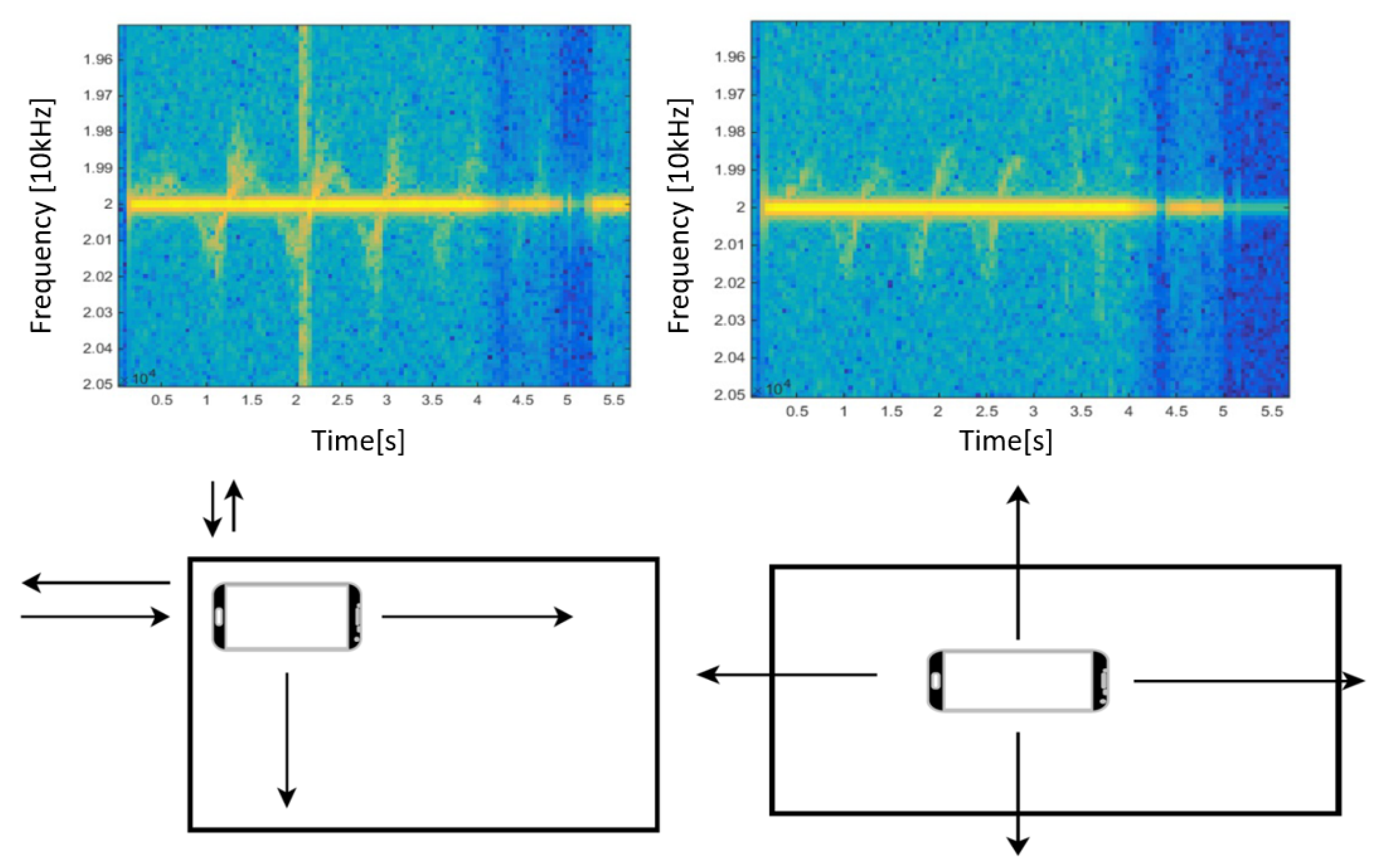
The best placement of the sensing device to obtain a strong back scattered signal is close to the wall or heading towards the corner of the wall. From both locations, we get enough reflections back to the device, which can be observed from the amplitude of the periodical frequency modulation around the center carrier frequency. The main reason is that the large ground plane also reflects the echo back to the device laying above. However, it can be observed that the placement close to the wall corner has the strongest back reflection. This is due to the Multi-path reflection additive from the corner of the wall. This effect of corner reflection has already be proven useful in radar applications [20]. A corner reflector is always used to calibrate the radar, since it has a very high radar-cross-section (RSC) or backscattering for a small size and the high RCS is maintained over a wide incidence angle. Therefore, in the case of our experiment, we collected our sports exercises data samples in near a wall, as depicted in Figure 1. We show this effect on a small experiment by placing the smartphone on a large desk and recording some simple waving gestures above the sensing device. We tested two different placing positions, which are in the middle of the table and on the edge of the table facing a corner of the wall. In each case, we either have no barriers due to the dimension of the device versus the large ground plane or have the same setup as a corner reflector. It can be clearly seen in Figure 2 that the placement on the corner close to the wall has the strongest back reflection.
In our previous work [10], we showed that back reflection of gestures performed on a mobile device put inside a trouser pocket is quite weak. The signal is weakened both ways, i.e., transmission and receiving. Thus, the measuring device should not be covered with clothes or towels. However, to obtain enough signal back propagation, we need to turn the volume of the sensing device to the maximum level. Occasionally, speaker and microphone are co-located, leading to unpredictable amplitude variations in the recording, which can cause problem for our processing algorithm. Furthermore, using the phone’s speakers at maximum output increases the amount of eigenfrequency excitation, which may fall into the human hearing range and thus disturb the user.

4. Classification Methods and Evaluation

We conducted a small field study to collect exercises data to test the different classification methods for our targeted application. We invited 14 participants ranging 25–28 years old to perform the three given sports activities. The 14 participants are grouped into 12 males and 2 females, with a weight ranging of 60–80 kg for males and 50–55 kg for females and a body height ranging 150–180 cm and 155–160 cm, respectively. We asked each participant to perform each activity fifteen times, which makes in total 45 samples per participant. The device we used to collect the activity data is a Google Nexus 5X. To condition the measurement setup, all exercises are performed in the same location. The exact placement can be seen in Figure 1.
For now, we implemented a mobile application to remotely annotate and collect the exercises data. The same application will be installed on two smartphones. This module can discover the peers registered under the same WiFi and connect them together. One device is used as a slave device to collect the data while users are performing sports activities close to it. The second device is used as a master device to remotely and manually label the activities performed. As for installation, there is no need for any external hardware. The data collection app has to be installed and running on the smartphone. It then can be placed on the ground and start to collect the echo of performed activities in the vicinity of the device. Since the backscattered signal is strongly dependent on the power emitted by the device itself, we have turned the device volume to the maximum level to assure enough signal back propagated by the reflection of the body. The signal strength should survive the two-way-paths.
For testing various classification schemes, we evaluated the data from the field test based on post-processing using Python and the scikit-learn library from Python [21] on a normal Desktop PC. We first pre-processed our data using the algorithm described in Section 2. We kept the preprocessing step simple, which only includes normalization and frequency band extraction. We then conditioned the collected data to compare these three different activities with each other. In Table 1, we can see the time duration of the fastest and slowest speeds of the performed activities.
We chose the average time performing each activity and thus have to inter- or extrapolate the collected data to make them into comparable data formats to feed them to the common classifiers. A simple linear interpolation scheme is used to condition the data. Therefore, the input data have the dimension of 186 × 40, ranging from frequency to time domain. The 186 frequency bins represent the frequency range of 19 kHz to 21 kHz and 40 time samples represent a duration of 1.85 s. For the current evaluation, the start and end markers are labeled manually. For later online application, the sliding window approach should be used to classify different sports exercises.
We then tested different classification schemes including Naive Bayes (NB), support vector machines (SVM), random forest (RF) and AdaBoost to evaluate the classification results. To perform the classification, we further divided all collected samples into 80% training samples and 20% test samples. This makes sure that the classifier has not seen the test samples before during the training phase. In this way, we can generalize the outcome of our classifier for unknown inputs. We also use the 10-fold cross-validation to show the macro-precision and the macro-recall to the different classification schemes. In the following section, we describe the evaluation results for all the different classifiers tested and try to offer the best suitable classifier for our intended application.

4.1. Classical Machine Learning Classification Schemes

Naive Bayes (NB) Classifier is built on the Bayes theorem. It is a supervised learning algorithm. The assumption here is that every feature pair is independent. It is the simplest form of Bayesian network. Bayes theorem provides a way to calculate the posterior probability P ( c | x ) from the probabilities P ( c ) , P ( x ) and P ( x | c ) of the sample distribution by applying Equation (2).
P ( c | x ) = P ( x | c ) P ( c ) P ( x )
where c stands for the class and x for the observation. Therefore, P ( c ) gives the probability of the class c and P ( x ) gives the probability of observing the feature representation x. The term P ( x | c ) denotes the conditional probability of making the observation x given the underlying class c and is thus the class conditional probability. The Naive Bayes classifier has been already used for Doppler based activity classification mostly as a baseline classifier, e.g., by Smith et al. [22] or Ritchie et al. [23].
Support vector machines (SVM) are known as a large margin linear classifier. A hyperplane separates the classes in the SVM algorithm. The SVM works by finding the maximized distance between the hyperplane boundaries. The distance between the boundaries is called the margin. However, unlike logistic regression for binary classification, the support vector machine does not provide probabilities, but only outputs a class identity. SVM can also classify non-linear data. The process of doing this is through a process called kernel trick. Here, the SVM transforms the non-linear data from a lower dimension to a higher dimension and tries to linearly separate the data there. SVM is, in general, a binary classification scheme, but it can be extended to a multi-classes algorithm by using the one-versus-rest or the one-versus-one method. The theory of SVM can be found in various textbooks [24].
Random Forests work by training many decision trees on random subsets of the features, then averaging out their predictions. Building a model on top of many other models is also called Ensemble Learning, and it is often a great way to reduce the problem of over-fitting. The performance of Random forest is always better than the individual decision trees they rely on. Since the underlying single classifiers are independent from each other, they can be trained individually and hence fasten the learning speed. This kind of Ensemble Learning is also called bagging.
AdaBoost: One way for a new predictor to improve its predecessor is to pay a bit more attention to the training instances that the predecessor under-fitted or wrongly classified. This results in new predictors focusing more and more on the difficult cases. It keeps going until the number of the predefined models is arrived and then the perfect linear combination is constructed to classify the underlying problem by using Equation (3).
H ( x ) = t = 1 T α t · h t ( x )
The weights are learned in the successive learning process. This technique is called boosting and is also a kind of Ensemble learning. The difference towards the bagging approach is that the underlying classifiers are not independent from each other and thus can only be processed sequentially. Here, we used AdaBoost as a representative of the boosting algorithm.

4.2. Evaluation and Comparison

The confusion matrix for different classifiers is given in Figure 3 using the same split on training and test data. Naive Bayes classifier has a very high misclassification rate for the class toe touches compared to the class bicycle and squats. It often got the class toe touches confused with the other two classes. The class squat has the highest classification accuracy of 90%, while the class bicycle follows with an accuracy of 79%. Although the confusion matrix for Random Forest shows a relatively high accuracy of 84% for the class of bicycle and 87% for the toe touch class, it still works poorly on the class of squat. The Hyperparameters for Random Forest are shown in Table 2. We use 300 different single estimators with the maximum tree depth of 100 to setup our classifiers.
The confusion matrix for Multi-classes SVM using the one-versus-rest classification shows clearly better results. In our case, we used a linear kernel and a regularization parameter to prevent our classifier from overfitting. The Hyperparameters to setup the support vector machine can be observed in Table 3. In this scenario, the misclassification problems between squats versus bicycle or toe-touches or the misclassification between toe touch versus squats or bicycle have been drastically reduced. We obtain an accuracy of 72% for bicycles, 82% for toe-touches and 82% for squats. The overall performance is more stable and the results are much better than the Naive Bayes classifier or the Random Forest. Despite the slightly higher accuracy for the class of toe touch in the Random Forest classifier, we still cannot expect the RF classifier to outperform the support vector machine.
For AdaBoost classifiers, we used 300 weak estimators to setup the hyper classifier. AdaBoost proves to be the better classifier compared to Random forest, as the confusion matrix is more balanced. The main diagonal shows relatively good results for all the three classes. The same accuracy of 72% was achieved for the classes squats and bicycle and an accuracy of 65% was achieved for the class toe touches. However, of all classifiers observed thus far, the AdaBoost shows superior performance to Random Forest and Naive Bayes. However, compared to the Support Vector Machine, this classifier showed worse results with a considerably higher computational load.
In statistics, a receiver operating characteristic curve (ROC curve) is used as a graphical plot to illustrate the diagnostic ability of a binary classifier system with varied decision thresholds. The ROC gives the relationship between the true positive rate and the false positive rate. The definition of true positive and false positive rate are given in Equations (4) and (5), respectively.
T P R = T P T P + F N
F P R = F P T N + F P
The representation of the terms true positive, false negative, false positive and true negative in Equations (4) and (5) can be viewed in Table 4.
The area under the ROC curve (AUC) further indicates the performance of the classifier. If there is no classifier that has an AUC under 0.5, then the closer the AUC is to 1, the better the classifier works.
It is clearly shown that the Naive Bayes classifier is a bad classifier for this kind of data as the classifier is only slightly better than random decisions. The ROC curve for the Random Forest classifier can be see in Figure 4. The curves are steeper than the ROC curve of the NB classifier, which again indicates that the Naive Bayes classifier works poorly. The same behaves for the area under curve, which intends that the RF is a better suited classifier than Naive Bayes for our data set. The performance of toe touch class and the bicycle class are quite similar and better than the class squats, as the area under curve is larger. The ROC curve for the Support Vector Machine shows the best result over all classifiers tested so far. The performance of all the three classes are quite similar, as the area under curve are nearly identical. This is a good sign for choosing Support Vector Machine as a robust classifier for our application. The ROC curve for the AdaBoost classifier can also be seen in Figure 4. The class bicycle performs the best, while the class toe touch and the class squats behave similarly. These classifiers are steeper than in the case for the Random Forest, but not equally good as in the case of the support vector machine.
To give a more generalized score for all the classifiers tested, we give the macro precision score and the macro recall score for the 10-fold cross-validation case in Table 5. The equation for precision and recall are given in Equations (6) and (7), respectively.
P = T P T P + F P
R = T P T P + F N
The macro-precision and the macro-recall are the average precision and recall for all the 10-fold cross-validation.
The macro-precision and macro-recall of the different classification results using leave one subject out cross-validation is depicted in Table 6. The leave one subject out cross-validation can further show the person-dependency characteristic of the classification methods and hence is more generalized.

4.3. Activity Recognition Based on Convolutional Neural Networks

Activity recognition based on neural networks is a new field that has recently emerged [25]. Various deep learning neural networks have been tested on time series data for human activity recognition. The CNN is very similar to ordinary neural networks. They are made up of neurons that have learnable weights and biases. The difference is that it only takes account of the spatial information from neighbouring nodes, which means that CNN also captures local dependencies. This property is of vital importance since for activity recognition the temporal actions are related. Another property of CNN is its scale invariance based on the pooling layer. It finds the correct features in different scale levels. This corresponds to human activities performed with different speed. Some actions might be short, whereas some may take much more time.
The model of the convolutional neural network we used in this paper is depicted in Figure 5. Lower layers extract low-level features, for example edges or curves, whereas higher layers extract more abstract features out of combinations of low-level features. The main advantage of using CNN is that the neural network can automatically extract useful features or structures based on the training data.
Input to the neural network is the 2D time–frequency (STFT) dataset of the dimension 186 × 40 and the output from the softmax layer are three nodes corresponding to the probability of each class. The input dimension is chosen such that it covers the frequency range from 19 kHz to 21 kHz and 40 time samples represent a time duration of 1.85 s. The higher the output probability is, the more probable it could belong to this class. The output of each of the softmax node can be expressed by Equation (8).
s o f t m a x ( z ) i = e x p ( z i ) j e x p ( z j )
where i represents one of the three possible classes and j = 1 . . n u m O f c l a s s e s . The sum of the output results in 1, which means the class with the highest probability suppresses the rest of the classes. The number of the output nodes are directly correlated to the number of classes needed. This means in our case that three classes are required for the three activities. In the lower network layer, we use multiple convolution filters to extract the local dependencies in the input layer. The size of the convolution filters connects only part of the input nodes to catch the local dependencies. Three maxpooling layers are used to extract features from three different scales, which represent different user speeds. After each max pooling layer, the size will be reduced to half of the previous size. It is like a pyramid that you are able to get features from different scale levels. The dropout layer is used as a regularization term for the network and helps the network to avoid over-fitting. The dropout layer before the final layer is set to 0.5 and the previous dropout layers are all set to 0.25. At higher network layer, one fully connected layer is used to connect all the learned features. The final layer returns the prediction of the final class classification. The second dense layer is the softmax layer, which outputs the probabilities of each class. The weights in each individual layer are learned and updated using RMSprop as Optimizer and ReLu Layer as activation layer. The equation for ReLu activation layer was introduced by Hinton et al. [26]. In this case, the gradient descent learns the weight at activation range only. The equation for RMSProp was also first introduced by Hinton et al. [27]. The learning rate for each weight is updated by dividing a running average of the magnitudes of recent gradients for that weight. The advantage is that it reduces the problem of overshooting from the global optimum and it makes the network quickly converges to the global optimum.
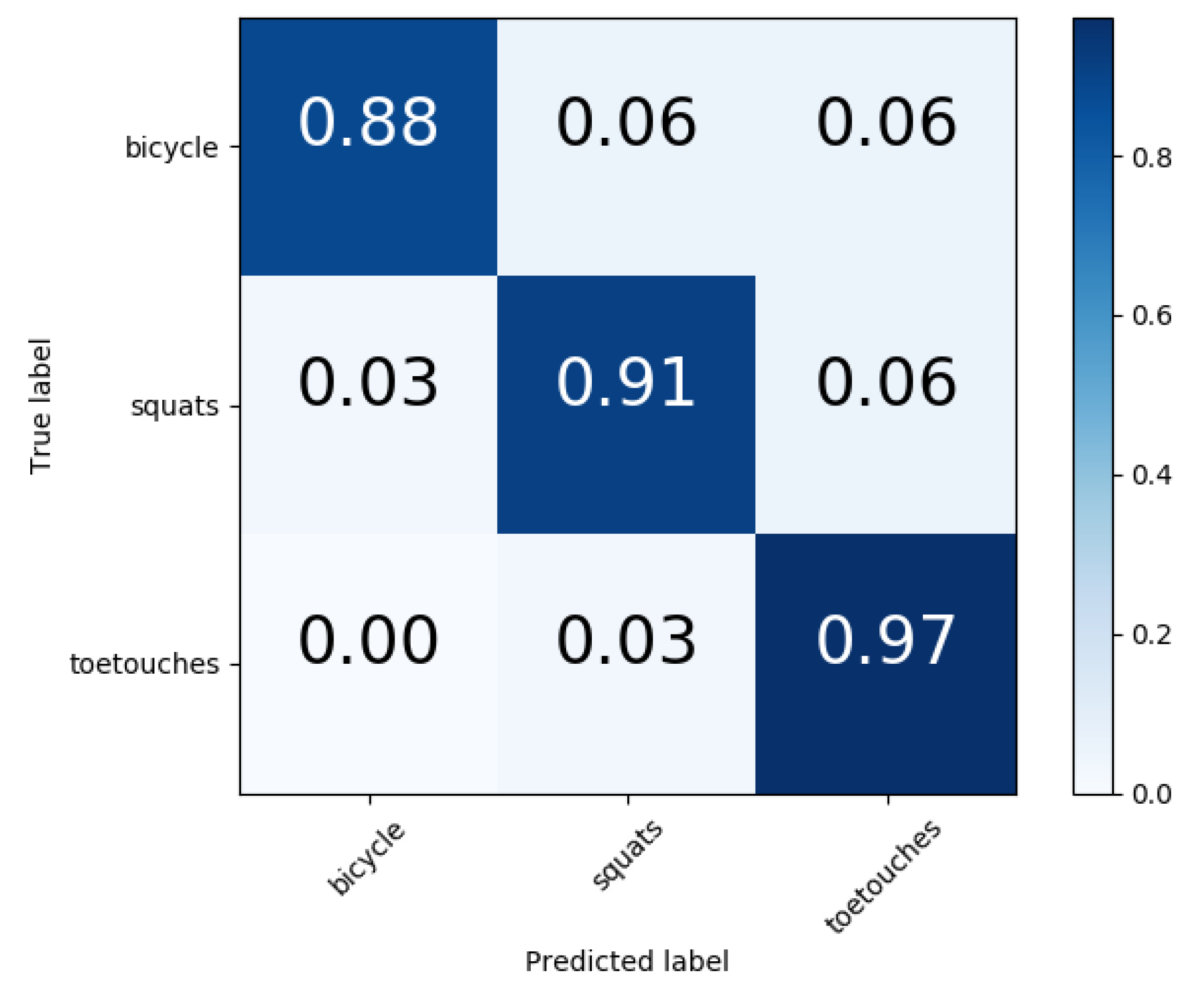
The confusion matrix for CNN applied to our collected exercise data can be see in Figure 6. The correct classification accuracy for all three classes are better than support vector machine. The misclassification rate are relatively low compared to the other classical machine learning approaches.

5. Conclusion and Outlook

In this study, we tested different classification methods including Naive Bayes, Support Vector Machine, Random Forest, AdaBoost and Convolutional Neural Network to evaluate up to three sports exercises recognition. We used only the built-in hardware components (microphone and speaker) of an unmodified consumer-grade smartphone. The sensing method was based on active sonar using the Doppler effect. The contributed concept could recognize the three different sports activities, i.e., bicycle, squats and toe touch, based on the evaluation done on collected samples. The evaluation was performed in postprocessing mode using Python with the scikit-learn package and the Tensorflow library for deep learning. The start and end markers were manually labeled and should be extended to use sliding window approach in the later online application. The choice of using an off-the-shelf unmodified smartphone to track sports activities was mostly due to its flexibility against wearable sensing devices or sensing technologies which need extra installations to the physical environment. Compared to visual input, e.g., the Kinect, it further preserve the privacy concern of the user. The preprocessing step is kept simple to test the generalized performance for all the classifiers despite the classical machine learning approaches like SVM or neural networks. First, the spectrogram in frequency–time domain was calculated and the frequency ranging between 19 kHz and 21 kHz over a time duration of 1.85 s was extracted. After applying a normalization step, the shape of the input data was constrained at 168 × 40 and within the amplitude range of [ 0 , 1 ] .
Different classifiers were used on the same training and testing samples and their 10-fold cross-validation results are given as the macro-precision and the macro-recall values. The confusion matrix and the ROC curve are depicted. The support vector machine showed the most robust and best performance compared to the other standard classical machine learning approaches with respect to the target application. We achieved an accuracy of 72% for the bicycle class, 82% for the squat class and 82% for the toe touches class. AdaBoost from Ensembled Learning also shows better performance than the Random Forest and the Naive Bayes, which is only slightly better than random guessing. However, compared to the SVM with an accuracy of 72% for bicycle and squats class and only 65% for toe touches, AdaBoost still needs much more computational effort for a worse result. Therefore, we conclude that the SVM performs the best compared to the other trained standard classifiers for our collected data set. We further showed that it is possible to even improve the accuracy by using a convolutional neural network. CNN shows its superior property of extracting features suitable for this kind of sport activity recognition, especially for the target three exercises. Due to its local dependencies between neighbouring nodes and its scale invariance, it performs extremely well on time series data such as ours. The final accuracy of our collected exercise data is about 88% for bicycle, 91% for squats and 97% for toe touches. The improvement of accuracy can be observed in all three classes.
However, it should be noted that all data collected in this paper has been created using a Google Nexus 5X. The placement of the device for the data collection is close to a wall. Different smartphone types can lead to different classification results due to the placement of microphones or the quality of hardware component used. Since the frequency range of speech is not considered, environmental noise is not a problem for the processing algorithm. In the future, we would try to expend the current method to more classes of exercise. Our research interest would also be in identifying users based on the activities performed.

Author Contributions

Biying Fu conceived and designed the experiment; Dinesh Vaithyalingam Gangatharan performed the experiments; Biying Fu analyzed the data and interpreted the analyzed results; Florian Kirchbuchner contributed materials to the related works; Biying Fu wrote the paper; and Arjan Kuijper and Andreas Braun helped by proofreading and commenting on the structure of the paper.

Conflicts of Interest

The authors declare no conflict of interest.

References

  1. Anderson, F.; Grossman, T.; Matejka, J.; Fitzmaurice, G. YouMove: Enhancing Movement Training with an Augmented Reality Mirror. In Proceedings of the 26th Annual ACM Symposium on User Interface Software and Technology, St. Andrews, UK, 8–11 October 2013; pp. 311–320. [Google Scholar]
  2. Velloso, E.; Bulling, A.; Gellersen, H. MotionMA: Motion Modelling and Analysis by Demonstration. In Proceedings of the SIGCHI Conference on Human Factors in Computing Systems, Paris, France, 27 April–2 May 2013; pp. 1309–1318. [Google Scholar]
  3. Kirchbuchner, F.; Grosse-Puppendahl, T.; Hastall, M.R.; Distler, M.; Kuijper, A. Ambient Intelligence from Senior Citizens’ Perspectives: Understanding Privacy Concerns, Technology Acceptance, and Expectations. In Ambient Intelligence; Springer: Berlin, Germany, 2015; pp. 48–59. [Google Scholar]
  4. Ding, H.; Shangguan, L.; Yang, Z.; Han, J.; Zhou, Z.; Yang, P.; Xi, W.; Zhao, J. FEMO: A Platform for Free-weight Exercise Monitoring with RFIDs. In Proceedings of the 13th ACM Conference on Embedded Networked Sensor Systems, Seoul, Korea, 1–4 November 2015; pp. 141–154. [Google Scholar]
  5. Mitchell, E.; Monaghan, D.; O’Connor, N.E. Classification of Sporting Activities Using Smartphone Accelerometers. Sensors 2013, 13, 5317–5337. [Google Scholar] [CrossRef] [PubMed] [Green Version]
  6. Schmidt, A. Implicit human computer interaction through context. Pers. Technol. 2000, 4, 191–199. [Google Scholar] [CrossRef]
  7. Lu, H.; Pan, W.; Lane, N.D.; Choudhury, T.; Campbell, A.T. SoundSense: Scalable Sound Sensing for People-centric Applications on Mobile Phones. In Proceedings of the 7th International Conference on Mobile Systems, Applications, and Services, Kraków, Poland, 22–25 June 2009; ACM: New York, NY, USA, 2009; pp. 165–178. [Google Scholar]
  8. Schweizer, I.; Bärtl, R.; Schulz, A.; Probst, F.; Mühlhäuser, M. NoiseMap-Real-time participatory noise maps. In Proceedings of the Second International Workshop on Sensing Applications on Mobile Phones, Seattle, WA, USA, 1–4 November 2011. [Google Scholar]
  9. Popescu, M.; Li, Y.; Skubic, M.; Rantz, M. An acoustic fall detector system that uses sound height information to reduce the false alarm rate. In Proceedings of the 30th Annual International Conference of the IEEE Engineering in Medicine and Biology Society, Vancouver, BC, Canada, 20–24 August 2008; pp. 4628–4631. [Google Scholar]
  10. Fu, B.; Karolus, J.; Grosse-Puppendahl, T.; Herrmann, J.; Kuijper, A. Opportunities for Activity Recognition using Ultrasound Doppler Sensing on Unmodified Mobile Phones. In Proceedings of the 2nd international Workshop on Sensor-based Activity Recognition and Interaction, Rostock, Germany, 25–26 June 2015. [Google Scholar]
  11. Gupta, S.; Morris, D.; Patel, S.; Tan, D. SoundWave: Using the Doppler Effect to Sense Gestures. In Proceedings of the SIGCHI Conference on Human Factors in Computing Systems, Austin, Texas, USA, 5–10 May 2012; pp. 1911–1914. [Google Scholar]
  12. Aumi, M.T.I.; Gupta, S.; Goel, M.; Larson, E.; Patel, S. DopLink: Using the Doppler Effect for Multi-device Interaction. In Proceedings of the 2013 ACM International Joint Conference on Pervasive and Ubiquitous Computing, Zurich, Switzerland, 8–12 September 2013; pp. 583–586. [Google Scholar]
  13. Sun, Z.; Purohit, A.; Bose, R.; Zhang, P. Spartacus: Spatially-aware Interaction for Mobile Devices Through Energy-efficient Audio Sensing. In Proceedings of the 11th Annual International Conference on Mobile Systems, Applications, and Services, Taipei, Taiwan, 25–28 June 2013; pp. 263–276. [Google Scholar]
  14. Yang, Q.; Tang, H.; Zhao, X.; Li, Y.; Zhang, S. Dolphin: Ultrasonic-Based Gesture Recognition on Smartphone Platform. In Proceedings of the 2014 IEEE 17th International Conference on Computational Science and Engineering (CSE), Chengdu, China, 19–21 December 2014; pp. 1461–1468. [Google Scholar]
  15. Ruan, W.; Sheng, Q.Z.; Yang, L.; Gu, T.; Xu, P.; Shangguan, L. AudioGest: Enabling Fine-grained Hand Gesture Detection by Decoding Echo Signal. In Proceedings of the 2016 ACM International Joint Conference on Pervasive and Ubiquitous Computing, Heidelberg, Germany, 12–16 September 2016; ACM: New York, NY, USA, 2016; pp. 474–485. [Google Scholar]
  16. Nandakumar, R.; Gollakota, S.; Watson, N. Contactless Sleep Apnea Detection on Smartphones. In Proceedings of the 13th Annual International Conference on Mobile Systems, Applications, and Services, Florence, Italy, 18–22 May 2015; ACM: New York, NY, USA, 2015; pp. 45–57. [Google Scholar]
  17. Nandakumar, R.; Iyer, V.; Tan, D.; Gollakota, S. FingerIO: Using Sonar for Fine-Grained Finger Tracking. In Proceedings of the SIGCHI Conference on Human Factors in Computing Systems, San Jose, CA, USA, 7–12 May 2016. [Google Scholar]
  18. Xi, W.; Huang, D.; Zhao, K.; Yan, Y.; Cai, Y.; Ma, R.; Chen, D. Device-free Human Activity Recognition Using CSI. In Proceedings of the 1st Workshop on Context Sensing and Activity Recognition, Seoul, Korea, 1 November 2015; pp. 31–36. [Google Scholar]
  19. Fu, B.; Gangatharan, D.V.; Kuijper, A.; Kirchbuchner, F.; Braun, A. Exercise Monitoring On Consumer smartphones Using Ultrasonic Sensing. In Proceedings of the 4th International Workshop on Sensor-based Activity Recognition and Interaction, Rostock, Germany, 21–22 September 2017; ACM: New York, NY, USA, 2017. [Google Scholar]
  20. Shan, X.J.; Yin, J.Y.; Yu, D.L.; Li, C.F.; Zhao, J.J.; Zhang, G.F. Analysis of artificial corner reflector’s radar cross section: A physical optics perspective. Arabian J. Geosci. 2013, 6, 2755–2765. [Google Scholar] [CrossRef]
  21. Pedregosa, F.; Varoquaux, G.; Gramfort, A.; Michel, V.; Thirion, B.; Grisel, O.; Blondel, M.; Prettenhofer, P.; Weiss, R.; Dubourg, V.; et al. Scikit-learn: Machine Learning in Python. J. Mach. Learn. Res. 2011, 12, 2825–2830. [Google Scholar]
  22. Smith, G.E.; Woodbridge, K.; Baker, C.J. Naíve Bayesian radar micro-doppler recognition. In Proceedings of the 2008 International Conference on Radar, Adelaide, SA, Australia, 2–5 September 2008; pp. 111–116. [Google Scholar]
  23. Ritchie, M.; Fioranelli, F.; Borrion, H.; Griffiths, H. Multistatic micro-doppler radar feature extraction for classification of unloaded/loaded micro-drones. IET Radar Sonar Navig. 2017, 11, 116–124. [Google Scholar] [CrossRef]
  24. Steinwart, I.; Christmann, A. Support Vector Machines; Springer Publishing Company, Incorporated: Berlin, Germany, 2008. [Google Scholar]
  25. Ronao, C.A.; Cho, S.B. Human Activity Recognition with Smartphone Sensors Using Deep Learning Neural Networks. Expert Syst. Appl. 2016, 59, 235–244. [Google Scholar] [CrossRef]
  26. Nair, V.; Hinton, G.E. Rectified Linear Units Improve Restricted Boltzmann Machines. In Proceedings of the 27th International Conference on International Conference on Machine Learning, Haifa, Israel, 21–24 June 2010; pp. 807–814. [Google Scholar]
  27. Tieleman, T.; Hinton, G. Lecture 6.5—RmsProp: Divide the gradient by a running average of its recent magnitude. COURSERA Neural Netw. Mach. Learn. 2012, 4, 26–31. [Google Scholar]
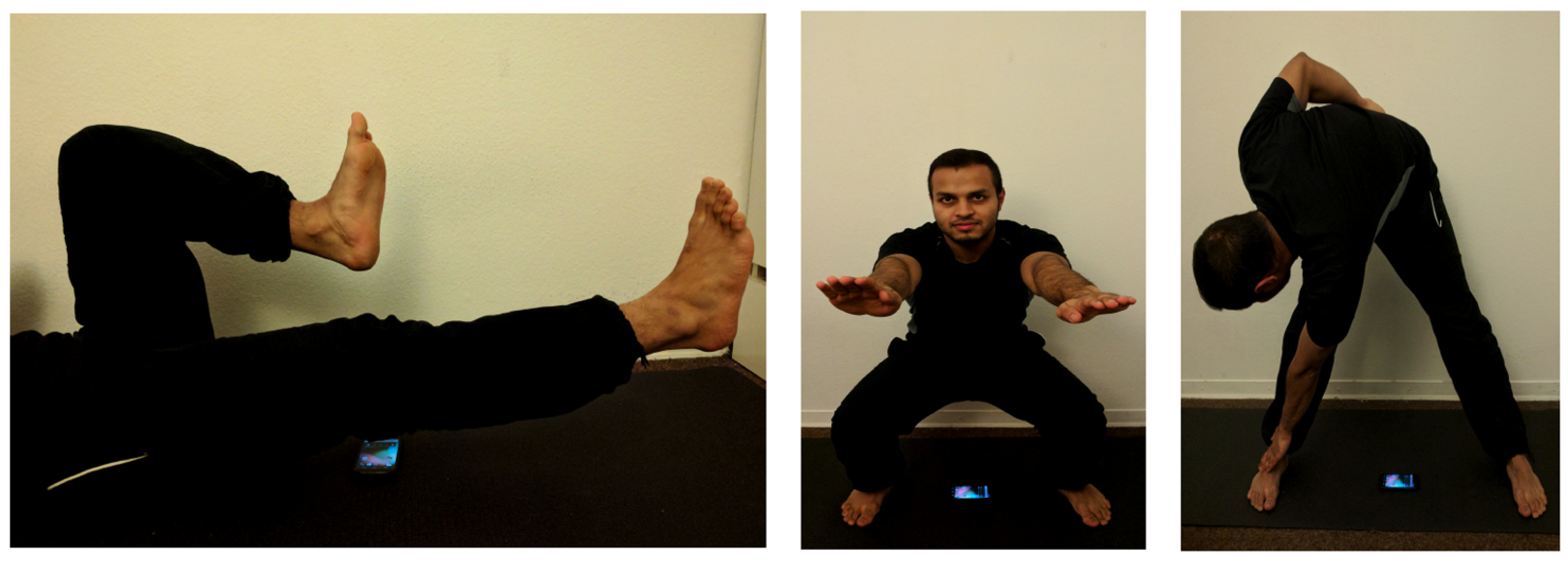
Figure 1. The three different sports activities monitored: bicycle exercise (left), squat exercise (middle) and toe touch exercise (right). The placement of the smartphone is close to the wall due to a stronger back-reflection.
Informatics 05 00024 g001
Figure 2. Bottom left shows the placement of the device on the corner of the table and its spectrogram is shown on the top left side. Bottom right: The device was placed in the middle of the table and its corresponding spectrogram is shown on the top right side. The back reflection of the corner placement is stronger due to the multi-path reflection.
Informatics 05 00024 g002
Figure 3. The confusion matrix for different classifiers are depicted. Top left (1) shows the confusion matrix for the Naive Bayes Classifier. Top right (2) shows the confusion matrix for the Random Forest classifier. Bottom left (3) shows the confusion matrix for the Support Vector Machine classifier. Bottom right (4) shows the confusion matrix for the AdaBoost classifier. As can be clearly seen from the results, AdaBoost classifier performs better than Naive Bayes and Random Forest. Although with higher computational load, it has a worse accuracy than support vector machine. The support vector machine shows the best recognition results with fewer misclassification rate.
Informatics 05 00024 g003
Figure 4. The ROC curve for different classifiers are depicted. Top left (1) shows the ROC curve for Naive Bayes Classifier. Top right (2) shows the ROC curve for the Random Forest classifier. Bottom left (3) shows the ROC curve for the Support Vector Machine classifier. Bottom right (4) shows the ROC curve for the Adaboost classifier. As can be extracted from the results, the Naive Bayes classifier performs the worst, which is only slightly better than random guessing. The Support Vector machine performs the best compared to the other classifiers. For all three classes, the ROC curves behaves similarly and shows the most robust results.
Informatics 05 00024 g004
Figure 5. The CNN Model used for our recognition task targeting three sports activities.
Informatics 05 00024 g005
Figure 6. Confusion matrix of the convolutional neural network is depicted.
Informatics 05 00024 g006
Table 1. The time duration for the fastest and slowest speed of each sports activities performed by the test participants. The abbreviation TS stands for time segment.
ExerciseMinimum (TS)Maximum (TS)Minimum Duration (s)Maximum Duration (s)
Bicycle13310.601.44
Squats12420.551.95
Toe touches11250.511.16
Table 2. Hyperparameters for Random Forest as a multi-Label classifier.
EstimatorsMax FeaturesTree Depth
300sqrt100
Table 3. Hyperparameters tuning for SVM as a multi-Label classifier.
Kernel γ Penalty Parameter
Linear0.00011
Table 4. The definition for different terms in Equations (4) and (5) are given.
True LabelPredicted Label
Positive SampleNegative Sample
Positive SampleTPFN
Negative SampleFPTN
Table 5. The macro-precision and macro-recall for the 10-fold cross-validation is presented here.
Naive BayesRandom ForestSupport Vector MachineAdaBoost
Precision64%77%84%77%
Recall61%68%83%75%
Accuracy60%72%83%76%
Table 6. The precision and recall using leave one subject out cross-validation is presented here.
Naive BayesRandom ForestSupport Vector MachineAdaBoost
Precision51%68%74%67%
Recall51%60%70%61%
Accuracy55%64%74%65%